The Indian financial sector has remained resilient building on the consolidation of the banking sector’s balance sheet, the ongoing reduction in bad loans and the buffering of risk absorbing capacity. Macro stress tests indicate that all banks would meet the regulatory minimum capital requirements even in a severe stress scenario. Stress tests indicate that some non-banking financial companies may be vulnerable to liquidity shocks. Contagion risks and consequent additional solvency losses remain limited. Introduction 2.1 The combination of regulatory measures undertaken to cushion banks since the onset of the pandemic and banks’ own efforts in augmenting their capital base and reducing non-performing loans appear to have fortified their balance sheets. A fresh lending cycle underway since H2:2021-22 gained further traction during H1:2022-23 as credit growth reached double digits and became broad based across sectors. Banks have managed their exposure to large borrowers well, with granularisation of loan books and reduction in asset impairment. 2.2 This chapter presents an evaluation of the soundness and resilience of financial intermediaries in India by analysing their recent performance on key parameters. Section II.1 presents an assessment of business mix, asset quality, capital adequacy, earnings and profitability of SCBs and evaluates their resilience against macroeconomic shocks through stress test and sensitivity analysis. Sections II.2 and II.3 examine the recent financial performance of urban cooperative banks (UCBs) and non-banking financial companies (NBFCs), respectively, and stress test their resilience. Sections II.4, II.5 and II.6 provide insights into the soundness and resilience of insurance, mutual funds, and clearing corporations, respectively. The concluding Section II.7 provides a detailed analysis of the network structure and connectivity of the Indian financial system and presents the results of contagion analysis under adverse scenarios. II.1 Scheduled Commercial Banks (SCBs)1 2 2.3 Aggregate deposits recorded some moderation, growing at 9.4 per cent as on December 16, 2022. Current account and savings account (CASA) growth moderated whereas term deposits attracted accretions in response to rising interest rates (Chart 2.1 a and b). 2.4 SCBs’ credit growth (y-o-y), which started picking up during H2:2021-22, sustained its momentum and gathered pace to touch a decadal high of 17.4 per cent as on December 16, 2022, a level last observed during 2011. The increase has been broad-based across geography, economic sectors, population groups, organisations, type of accounts and bank groups (Table 2.1 a and b). 2.5 PVBs continued to record much higher credit growth than PSBs (Chart 2.1 c). The share of services and personal loans3 in total advances inched up (Chart 2.1 d) with credit growth outpacing growth in agriculture and industry advances (Chart 2.1 e). Within personal loans segment, credit growth became broad based with credit card receivables and vehicle/ auto loans growing over 20 per cent (Chart 2.1 f). 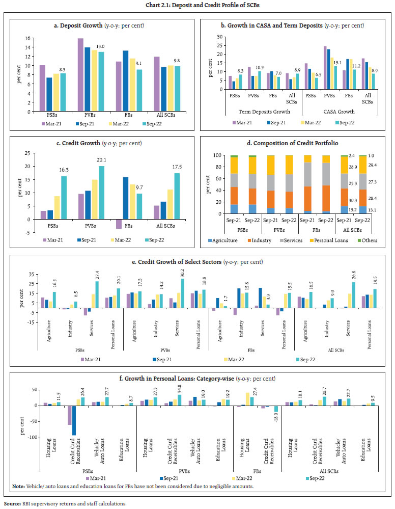
| Table 2.1 a: Credit Share and Growth* – September 2022 | | (per cent) | | Sector | | Share in total credit | Credit Growth (y-o-y) | | Organisational Sector | Public Sector | 16.7 | 15.6 | | Private Corporates | 26.3 | 14.7 | | Households - Individual | 44.4 | 19.6 | | Households – Others | 10.1 | 18.0 | | Other sectors | 2.5 | 52.0 | | Type of Account | Working capital loans | 32.7 | 16.5 | | Term loans | 64.0 | 19.5 | | Other Type of loans | 3.3 | 7.0 | | Population Group | Rural | 7.6 | 12.8 | | Semi-urban | 13.2 | 17.5 | | Urban | 16.8 | 20.3 | | Metropolitan | 62.4 | 18.2 | | Geographical Region | Northern | 21.2 | 14.8 | | North-Eastern | 1.1 | 17.4 | | Eastern | 7.1 | 17.7 | | Central | 8.9 | 19.7 | | Western | 33.2 | 22.1 | | Southern | 28.5 | 15.6 | Note: * excluding regional rural banks (RRBs).
Source: Basic Statistical Returns – 1 and staff calculations. | II.1.1 Asset Quality 2.6 The GNPA4 ratio of SCBs continued to decline and stood at a seven-year low of 5.0 per cent in September 2022. The net non-performing assets (NNPA)5 ratio stood at a ten-year low of 1.3 per cent, wherein PVBs’ NNPA ratio was below 1 per cent (Chart 2.2 a and b). The quarterly slippage ratio, which had been rising since December 2021, cooled off during Q2:2022-23, with considerable improvement recorded by PSBs (Chart 2.2 c). The provisioning coverage ratio (PCR)6 has been increasing steadily since March 2021, and reached 71.5 per cent in September 2022. The PCRs of PVBs and FBs exceeded 75 per cent (Chart 2.2 d). Meanwhile, the write-offs to GNPA ratio7 increased during H1:2022-23 on an annualised basis, after declining for two consecutive years (Chart 2.2 e). | Table 2.1 b: Growth in New Loans by SCBs: Economic Sectors, Organisations and Account type* | | (per cent) | | Sector | Q2: 2021-22 | Q3: 2021-22 | Q4: 2021-22 | Q1: 2022-23 | Q2: 2022-23 | | Growth (y-o-y) | | Economic sector wise | | Agriculture | 5.7 | 22.4 | 26.3 | 68.3 | 26.8 | | Industry | 5.6 | 19.6 | 13.6 | 22.5 | 27.9 | | Services | 3.3 | 20.0 | 15.7 | 49.9 | 34.8 | | Personal loans | 36.8 | 17.5 | 23.2 | 83.9 | 27.5 | | Organisation wise | | Public sector | -0.1 | 23.8 | 18.5 | 44.7 | 36.9 | | Private corporate sector | 12.2 | 17.4 | 14.6 | 29.3 | 25.6 | | Household sector | 17.7 | 19.4 | 20.6 | 77.9 | 27.2 | | of which, Individuals | 26.7 | 18.4 | 20.2 | 80.3 | 26.2 | | Other sectors | -9.0 | 36.0 | 54.8 | 50.2 | 103.0 | | Type of Account wise | | Working capital loans | 4.3 | 18.8 | 15.9 | 43.9 | 31.6 | | Term loans | 14.0 | 20.2 | 23.5 | 69.0 | 35.3 | | Other types of loans | 33.9 | 24.6 | 3.2 | 8.3 | 0.0 | | All new loans | 11.2 | 20.0 | 18.4 | 49.3 | 30.1 | | New loans in total loans (Share) | 15.1 | 16.8 | 17.9 | 15.2 | 16.6 | Note * excluding regional rural banks (RRBs).
Source: Basic Statistical Returns – 1 and staff calculations. |
II.1.2 Sectoral Asset Quality 2.7 SCBs’ asset quality continued to improve across most sectors (Chart 2.3 a). Improvement in the GNPA ratio in respect of the industrial sector also continued, although it remained elevated for gems and jewellery and construction sub-sectors (Chart 2.3 b). The asset quality of the personal loans segment improved during H1:2022-23, especially for housing and vehicle loans (Chart 2.3 c). II.1.3 Credit Quality of Large Borrowers8 2.8 The share of large borrowers in gross advances of SCBs has been on a declining path and their share in total GNPA has come down to 62.2 per cent in September 2022 from 75.6 per cent two years earlier (Chart 2.4 a). The GNPA ratio of large borrowers continued to improve and stood at 6.4 per cent in September 2022 from over 10 per cent in March 2021 (Chart 2.4 b). SMA-0 and SMA-29 loans of large borrowers had increased during Q1:2022-23, but it moderated in the latest quarter, implying containment of fresh slippages (Chart 2.4 c). The SMA-2 ratio recorded some increase but remained contained at 0.4 per cent in September 2022 (Chart 2.4 d). In the large borrower accounts, the proportion of standard assets in the total funded amount outstanding improved considerably from 86.2 per cent in March 2020 to 92.1 per cent in September 2022 with corresponding declines in NPAs. While there was an increase in the share of restructured standard advances from March 2020 to March 2022, the same have moderated during H1:2022-23 (Chart 2.4 e). 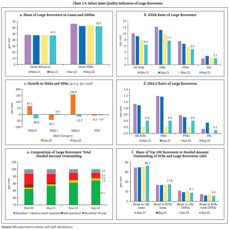 2.9 The share of top 100 large borrowers in the total loan book of SCBs continued to rise and stood at 17.4 per cent in September 2022, signalling fresh borrowing by large corporates. The asset quality of top 100 borrowers also improved considerably, as their share in SCBs’ GNPA declined from 6.8 per cent in March 2022 to 5.4 per cent in September 2022 (Chart 2.4 f). II.1.4 Capital Adequacy 2.10 The capital to risk weighted assets ratio (CRAR) of SCBs declined by 77 bps from March 2022 level on account of increase in risk weighted assets (RWAs) as lending activity picked up during H1:2022-23 (Chart 2.5 a). The system level TierI leverage ratio10 remained stable (Chart 2.5 b). II.1.5 Earnings and Profitability 2.11 At the system level, the net interest margin (NIM) witnessed an improvement of 20 bps between September 2021 and September 2022, reflecting a faster rate of increase in loan rates vis-à-vis deposit rates in a rising interest rate scenario as well as reduction in credit costs (Chart 2.6 a). Profit after tax (PAT) grew 40.7 per cent in September 2022, led by strong growth in net interest income (NII) and significant lowering of provisions. For the quarter ended September 2022, the PAT of PVBs grew by 60.7 per cent (y-o-y) as NII registered double digit growth and provisions almost halved (Chart 2.6 b). 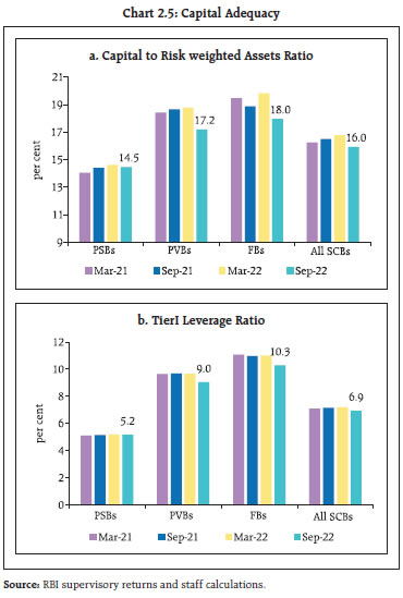 2.12 Return on equity (RoE) and return on assets (RoA) continued to improve to reach 11.2 per cent and 1.0 per cent, respectively, in September 2022 (Chart 2.6 c and d). After declining continuously over the last two years, the cost of funds increased and yield on assets improved (Charts 2.6 e and f). An analysis of the impact of rising G-sec yield on bank profitability in India suggests that the financial intermediation channel helps banks to attain higher profit even during an upward interest rate cycle (Box 2.1). 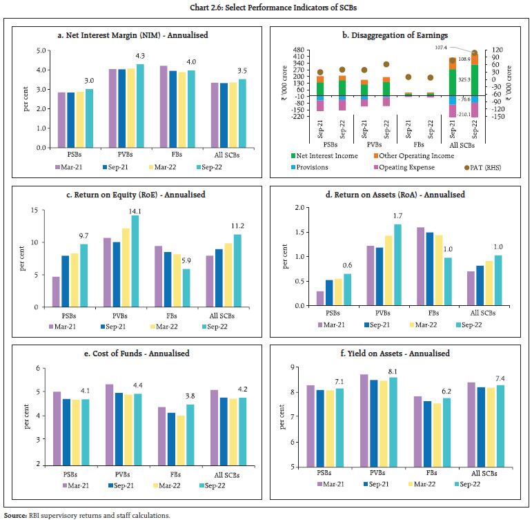
Box 2.1: Gilt Valuations and Bank Profitability Government securities (G-secs), including Treasury Bills (T-Bills) and State Development Loans (SDLs), amounted to about 81 per cent of the investment portfolio of scheduled commercial banks (SCBs) in September 2022 (Chart 1). Historically, public sector banks (PSBs) have maintained higher investments in G-secs than private sector banks (PVBs). In a monetary policy tightening cycle, rising yields impact trading income adversely on account of valuation losses. Banks’ trading income has in fact recorded large swings during the last five years (Chart 2). The effect of movements in yields differs across banks and also depends on the use of risk management techniques by banks to hedge interest rate risk in their trading book through derivatives. Banks’ net interest margins (NIMs) are also impacted by the slope11 of the yield curve - a steeper slope will mean a larger margin and higher profits for banks. The level and slope of yield curve affect the NIM and trading income in opposite directions, which is consistent with banks hedging interest rate risk (Alessandri and Nelson, 2015; Borio et al, 2017). In order to assess the impact of rising yields on bank profitability in India, a fixed effects panel data regression model covering 42 banks (PSBs and PVBs) for the period Q1:2015-16 to Q1:2022-23 was used (Table 1). Short-term yields and the slope of the yield curve are found to have a negative impact on trading income, reflecting the mark to market losses in the bond portfolio of banks, but the impact on NIMs is positive. Overall, it is found that interest income and other non-interest income (such as, fee and commission, underwriting, income from forex operations) can partly offset treasury losses in a rising interest rate scenario. | Table 1: Panel Regression – G-Sec Yield and Bank Profitability | | | Trading income/ total income | NIM | Operating Profit/Total Assets | | 1 | 2 | 3 | 4 | | NIM (-1) | | 0.487*** | | | | | (0.019) | | | T-bill (-1) | -1.015*** | 0.019** | 0.013*** | | | (0.137) | (0.009) | (0.004) | | Slope (-1) | -1.968*** | 0.015 | | | | (0.178) | (0.014) | | | GNPA Ratio | | -0.008*** | -0.004*** | | | | (0.002) | (0.001) | | CASA/total deposits | | 0.008*** | 0.003*** | | | | (0.002) | (0.001) | | Cost-income ratio | | -0.004*** | -0.009*** | | | | (0.001) | (0.001) | | Spread | | 0.396*** | 0.013*** | | | | (0.016) | (0.001) | | Liquid assets/total assets | | -0.007*** | -0.002 | | | | (0.002) | (0.001) | | CPI inflation | -0.017 | 0.012*** | 0.003 | | | (0.057) | (0.004) | (0.002) | | Leverage ratio | 0.223** | | 0.009** | | | (0.106) | | (0.004) | | Covid dummy | 1.171*** | | -0.004 | | | (0.275) | | (0.011) | | Merger dummy | | 0.198*** | 0.057*** | | | | (0.054) | (0.008) | | Constant | 9.314*** | 0.433*** | 0.462*** | | | (1.297) | (0.116) | (0.079) | | Observations | 880 | 1,122 | 880 | | Number of bank | 42 | 42 | 42 | | R-squared | 0.164 | 0.818 | 0.544 | | Bank Fixed Effect | Yes | Yes | Yes | Note: Standard errors in parentheses
*** p<0.01, ** p<0.05, * p<0.1 | Countercyclical macroprudential tools such as the investment fluctuation reserve (IFR) created by transferring the gains realised on sale of investments during easing interest rate cycle, act as a shock absorber in a tightening phase. The IFR guidelines were revised in April 2018 under which banks were advised to transfer net profit on sale of investment to the IFR, until it reaches at least two per cent of the Held for Trading (HFT) and Available for Sale (AFS) portfolios and, where feasible, this should be achieved within a period of three years. The banking system’s IFR reached 2.2 per cent of HFT + AFS portfolios in March 2022 (Chart 3). This has helped banks to absorb the losses associated with the rise in G-sec yields in Q1:2022-23 and resultant treasury losses, to the tune of 4.9 per cent of their operating profit. However, banks reported positive trading income to the tune of 2.1 per cent of operating profit as G-sec yield plateaued in Q2:2022-23. 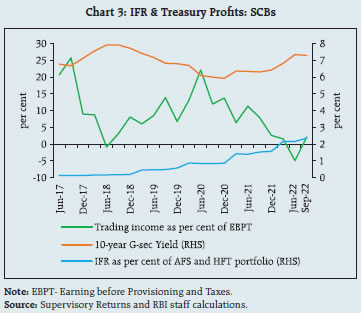 Central banks are confronting elevated inflation by tightening monetary conditions, which leaves banks exposed to fluctuations in G-sec yields but the countercyclical IFR is expected to provide a buffer against valuation losses in their investment portfolio. References 1. Alessandri, P. and B. D. Nelson (2015). Simple Banking: Profitability and the Yield Curve. Journal of Money, Credit and Banking, 47(1), 143–175. 2. Borio, C., L. Gambacorta, and B. Hofmann (2017). The Influence of Monetary Policy on Bank Profitability. International Finance, 20(1):48-63. | II.1.6 Resilience – Macro Stress Tests 2.13 Macro-stress tests are performed to assess the resilience of SCBs’ balance sheets to unforeseen shocks emanating from the macroeconomic environment. These tests attempt to assess capital ratios over a one-year horizon under a baseline and two adverse12 (medium and severe) scenarios. The baseline scenario is derived from the forecasted values of macro variables. The medium and severe adverse scenarios are arrived at by applying 0.25 to one standard deviation (SD) shocks and 1.25 to two SD shocks, respectively, to the macroeconomic variables, increasing the shocks sequentially by 25 basis points in each quarter (Chart 2.7). 2.14 Stress test results reveal that SCBs are well capitalised and capable of absorbing macroeconomic shocks even in the absence of any further capital infusion by stakeholders. Under the baseline scenario, the aggregate CRAR of 46 major banks is projected to slip from 15.8 per cent in September 2022 to 14.9 per cent by September 2023. It may go down to 14.0 per cent in the medium stress scenario and to 13.1 per cent under the severe stress scenario by September 2023, but it stays well above the minimum capital requirement, including capital conservation buffer (CCB) requirements (11.5 per cent) (Chart 2.8 a). None of the 46 SCBs would breach the regulatory minimum capital requirement of 9 per cent in the next one year, even in a severely stressed situation, although 9 SCBs may fall short of the minimum capital inclusive of CCB (Chart 2.8 b). 2.15 The CET1 capital ratio of the select 46 SCBs may decline from 12.8 per cent in September 2022 to 12.1 per cent by September 2023 under the baseline scenario (Chart 2.9 a). Even in a severely stressed macroeconomic environment, the aggregate CET1 capital ratio would deplete only by 210 basis points, which would not breach the minimum regulatory norms. Furthermore, all the banks would be able to meet the minimum regulatory CET1 ratio plus CCB of 8.0 per cent over the next one year under all the three scenarios (Chart 2.9 b). 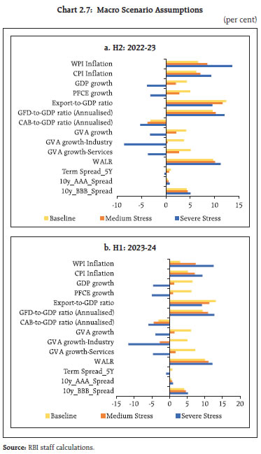
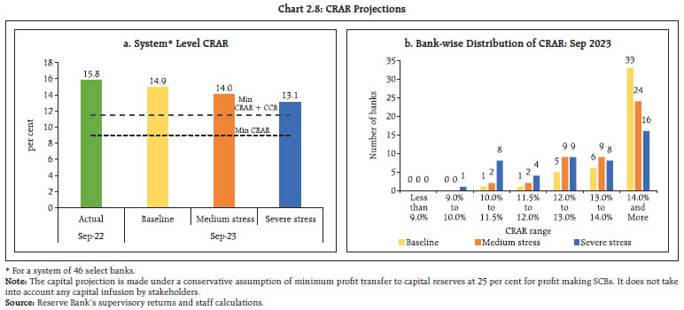
2.16 The decrease in slippage, increase in write-offs and the continuous improvement in loan growth brought the GNPA ratio further down to 5.0 per cent in September 2022. Under the assumption of no further regulatory reliefs as well as without taking the potential impact of stressed asset purchases by National Asset Reconstruction Company Limited (NARCL) into account, stress tests indicate that the GNPA ratio of all SCBs may improve from 5.0 per cent in September 2022 to 4.9 per cent by September 2023, under the baseline scenario (Chart 2.10). If the macroeconomic environment worsens to a medium or severe stress scenario, the ratio may rise to 5.8 per cent and 7.8 per cent, respectively. At the bank group level, the GNPA ratios of PSBs may swell from 6.5 per cent in September 2022 to 9.4 per cent in September 2023, whereas it would go up from 3.3 per cent to 5.8 per cent for PVBs and from 2.5 per cent to 4.1 per cent for FBs, under the severe stress scenario. 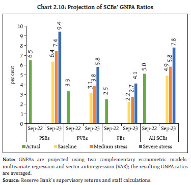 II.1.7 Sensitivity Analysis13 2.17 Top-down14 sensitivity analysis involving several single-factor shocks to simulate credit, interest rate, equity price and liquidity risks under various stress scenarios15 were carried out to assess the vulnerabilities of SCBs based on their operations up to September 2022. a. Credit Risk 2.18 Credit risk sensitivity has been analysed under two scenarios wherein the system-level GNPA ratio is assumed to rise by (i) one SD16 and (ii) two SDs from its prevailing level in a quarter. Under a severe shock of two SDs in which the aggregate GNPA ratio of 46 select SCBs moves up from 5.1 per cent to 10.0 per cent, the system-level CRAR would deplete by 350 bps from 15.8 per cent to 12.3 per cent and the Tier I capital ratio from 13.7 per cent to 10.2 per cent, but would remain well above the regulatory minimum. The system-level capital impairment could be 23.5 per cent in this case (Chart 2.11 a). The reverse stress test shows that it requires a shock of 4.4 SD to bring down the system-level CRAR to the regulatory minimum of 9 per cent. However, a shock of 2.5 SD can bring down the system-level CRAR below the regulatory minimum CRAR inclusive of the CCB, which totals 11.5 per cent. 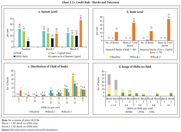 2.19 Bank-level stress test results show that under the severe (two SD) shock scenario, 11 banks with 22.5 per cent share in SCBs’ total assets may fail to maintain the regulatory minimum level of CRAR (Chart 2.11 b). In such a scenario, the CRAR would fall below 7 per cent in case of seven banks (Chart 2.11 c) and six banks would record a decline of over eight percentage points in the CRAR. In general, PVBs and FBs would face lower erosion in CRAR than PSBs under both scenarios (Chart 2.11 d). b. Credit Concentration Risk 2.20 Stress tests on banks’ credit concentration – considering top individual borrowers according to their standard exposures – showed that in the extreme scenario of the top three individual borrowers of respective banks failing to repay17, no bank will face a drop in CRAR below the regulatory requirement of 9 per cent, although three banks would see a decline in CRAR below 11.5 per cent - the regulatory minimum inclusive of CCB (Chart 2.12 a). In this case, twelve banks would experience a fall of more than two percentage points in their CRARs (Chart 2.12 b). 2.21 Under the extreme scenario of the top three group borrowers in the standard category failing to repay18, CRARs of all banks would remain above 9 per cent, but five banks may fail to meet the regulatory minimum inclusive of CCB (Chart 2.13 a) and two banks may face a decline of more than five percentage points in CRARs (Chart 2.13 b).
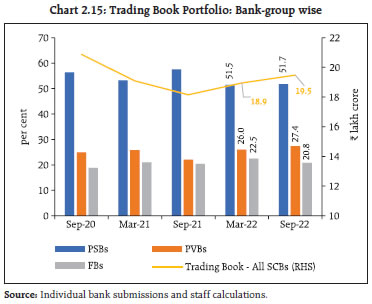
2.22 In the extreme scenario of the top three individual stressed borrowers of respective banks failing to repay19, the majority of the banks would remain resilient, with their CRARs depleting by mere 25 bps or lower (Chart 2.14). c. Sectoral Credit Risk 2.23 Shocks applied on the basis of volatility of industry sub-sector wise GNPA ratio indicate varying magnitudes of increases in banks’ GNPAs in different sub-sectors. A two SD shock to metals and energy sub-sectors reduces the system-level CRAR by 16 bps (Table 2.2). d. Interest Rate Risk 2.24 The market value of investments subject to fair value stood at ₹19.5 lakh crore in September 2022 for the sample of SCBs under review (Chart 2.15). 95.7 per cent of these investments were classified as ‘available for sale (AFS)’ and the remaining were under the ‘held for trading (HFT)’ category. The share of PSBs, which hold more than half of the total trading book portfolio of SCBs, has increased marginally in H1:2022-23. 2.25 The sensitivity (PV0120) of the AFS portfolio decreased for PSBs vis-à-vis the June 2022 position whereas it increased for PVBs and FBs. In terms of PV01 curve positioning, the tenor-wise distribution of PSBs’ portfolio indicated higher allocation in the 5-10 year bucket and in the more than 10-year bucket, compared to June 2022. Around four-fifth of PSBs’ AFS portfolio are in the 1-5 year and 5-10 year buckets. Similarly, PVBs have built up their position in the more than 10-year bucket and 5-10 year bucket, while paring allocations in less than 1 year and 1-5 year buckets. FBs continue to prefer the more than 10-year bucket, while concomitantly increasing their holding in other buckets. Although PV01 exposure of FBs in the highest maturity segment remains substantial, it may not be an active contributor to risk as some positioning involves bonds held as cover for hedging derivatives (Table 2.3). | Table 2.2: Decline in System Level CRAR | | (basis points, in descending order for top 10 most sensitive sectors) | | | 1 SD | 2 SD | | Basic Metal and Metal Products (389%) | 9 | 16 | | Infrastructure - Energy (172%) | 8 | 16 | | Infrastructure – Transport (48%) | 3 | 6 | | Construction (30%) | 2 | 5 | | Food Processing (28%) | 2 | 4 | | Infrastructure - Communication (104%) | 1 | 3 | | Gems and Jewellery (33%) | 1 | 2 | | Cement and Cement Products (95%) | 1 | 2 | | Petroleum (non-infra), Coal Products (non-mining) and Nuclear Fuels (203%) | 1 | 2 | | Mining and Quarrying (93%) | 1 | 2 | Note: For a system of select 46 banks.
Numbers in parentheses represent the growth in GNPA of that sub-sector due to 1 SD shock to the sub-sector’s GNPA ratio.
Source: RBI supervisory returns and staff calculations. |
| Table 2.3: Tenor-wise PV01 Distribution of AFS Portfolio | | | Total
(in ₹ crore) | Share (in per cent) | | <1 year | 1-5 year | 5-10 year | >10 years | | PSBs | 191.9
(219.5) | 8.6
(14.5) | 36.9
(40.1) | 46.9
(38.6) | 7.7
(6.9) | | PVBs | 63.0
(55.1) | 20.1
(32.5) | 42.9
(43.5) | 12.5
(7.6) | 24.5
(16.4) | | FBs | 138.6
(132.1) | 4.1
(3.7) | 17.4
(17.4) | 17.9
(15.3) | 60.6
(63.5) | Note: Values in the parentheses indicate June 2022 figures.
Source: Individual bank submissions and staff calculations. | 2.26 As on December 7, 2022 the sovereign yield curve has flattened with the short end of the curve moving up sharply relative to June 2022. Concomitantly, the systemic surplus liquidity has come down from ₹6.35 lakh crore as on April 1, 2022 to ₹1.62 lakh crore as of December 7, 2022. 2.27 Nevertheless, the yield curve has moved down on December 7, 2022 as compared to its position in September 2022, facilitated in large measure by the easing of inflation and the prospect of subdued government borrowing in the wake of robust tax revenues (Chart 2.16). 2.28 Trading profits of PSBs and PVBs returned to positive territory in Q2:2022-23 after reporting losses in Q1:2022-23. Although trading losses continued for the seventh consecutive quarter for FBs, it has reduced from March 2022 levels. The share of trading profits in net operating income was miniscule for PSBs and PVBs, while it dampened net operating income for FBs (Table 2.4). 2.29 In the HFT portfolio, the interest rate exposure of PVBs and FBs remained higher than that of PSBs, but all three bank groups converged in their trading strategies and interest rate outlook. PSBs have initiated a net positive position in their HFT books in Q2:2022-23 after having a fully squared position in June 2022. PVBs and FBs have decreased their sensitivity (PV01) in the HFT portfolio. PSBs have built up their long positions in the 5-10 year bucket relative to their short position in the same bucket during June quarter. They have pared their positions in the less than 1 year and 1-5 year buckets. PVBs and FBs have built up positions in the 1-5 year and more than 10-year buckets while reducing their position in the 5-10 year bucket (Table 2.5). 2.30 It is assessed that a parallel upward shift of 250 bps in the yield curve would reduce the system level CRAR by 73 bps. Analogously, the system level CET1 capital would decline by 76 bps (Table 2.6). At a disaggregated level, no bank would face a situation in which the CRAR and CET1 ratios fall below the regulatory minimum, although a few foreign banks could face substantial erosion in their capital in a stressed scenario.
| Table 2.4: Other Operating Income (OOI) - Profit/(Loss) on Securities Trading | | (in ₹ crore) | | | Q2: 2021-22 | Q3: 2021-22 | Q4: 2021-22 | Q1: 2022-23 | Q2: 2022-23 | | PSBs | 5765
(13.9) | 3023
(6.4) | 2457
(4.3) | -3465
(-8.0) | 2376
(2.4) | | PVBs | 1996
(4.4) | 573
(1.2) | 1162
(2.3) | -643
(-1.3) | 471
(0.4) | | FBs | -204
(-2.6) | -874
(-11.2) | -1668
(-13.9) | -903
(-9.5) | -233
(-1.3) | Note: Figures in parentheses represent OOI-Profit/(Loss) as a percentage of Net Operating Income.
Source: RBI Supervisory Returns. |
| Table 2.5: Tenor-wise PV01 Distribution of HFT portfolio | | | Total
(₹ crore) | Share (in per cent) | | <1 year | 1-5 year | 5-10 year | >10 years | | PSBs | 1.5
(0.0) | 2.4
(148.6) | 5.0
(192.7) | 86.1
(-215.1) | 6.4
(-26.2) | | PVBs | 15.0
(24.5) | 1.2
(4.7) | 22.6
(3.2) | 44.4
(92.3) | 31.7
(-0.2) | | FBs | 8.3
(9.8) | 8.4
(6.8) | 34.4
(21.3) | 31.9
(54.2) | 25.3
(17.7) | Note: Values in the brackets indicate June 2022 figures.
Source: Individual bank submissions and staff calculations. | 2.31 PSBs preferred to pare their allocation in G-secs and increased their holdings of SDLs and other securities eligible for holding in the HTM category (Chart 2.17). PVBs increased their holding of G-secs and SDLs, while decreasing the holding of other securities in the HTM category. 2.32 Unrealised losses of PSBs were largely in G-sec, although the proportion of central and state government securities held by them in the HTM portfolio were, by and large, equal. PVBs’ losses were largely distributed in proportion of their holdings (Chart 2.18). For a 250 bps parallel upward shift of the yield curve, the impact on the HTM portfolio of banks, if marked to market, would cause the system level CRAR to reduce by 307 bps. 2.33 In September 2022, holding of statutory liquidity ratio (SLR) securities by PSBs and PVBs in the HTM category amounted to 21.4 per cent and 19.9 per cent, respectively, of their net demand and time liabilities (NDTL), while it stood at 2.9 per cent for FBs. The expected paring of HTM book by banks as credit growth started to gather pace has not materialised. In fact, PSBs and PVBs have increased their HTM book albeit marginally. 2.34 An assessment of the interest rate risk in banking book21 (IRRBB) using Traditional Gap Analysis (TGA), for time buckets up to one year, shows that Earnings at Risk (EAR) would be impacted by a little above 10 per cent of NII for PSBs and PVBs and marginally for FBs and small finance banks (SFBs) in case of a 200 bps increase in interest rate (Table 2.7). The impact is positive for increase in interest rate as the cumulative gap22 at bank group level was positive as of September 2022. | Table 2.6: Interest Rate Risk – Bank-groups - Shocks and Impacts | | (under shock of 250 basis points parallel upward shift of the INR yield curve) | | | Public Sector Banks | Private Sector Banks | Foreign Banks | All SCBs | | AFS | HFT | AFS | HFT | AFS | HFT | AFS | HFT | | Modified Duration (year) | 1.9 | 4.0 | 1.3 | 3.7 | 3.8 | 2.1 | 2.1 | 2.9 | | Share in total Investments (per cent) | 30.3 | 0.1 | 30.5 | 1.4 | 86.1 | 7.9 | 35.2 | 1.2 | | Reduction in CRAR (bps) | 67 | 34 | 280 | 73 | | Reduction in CET1 Capital (bps) | 70 | 35 | 286 | 76 | | Source: Individual bank submissions and staff calculations. |
2.35 IRRBB analysis using Duration Gap Analysis (DGA)23 reveals that PVBs’ and FBs’ Market Value of Equity (MVE) would reduce marginally by an upward movement in interest rate, while that of PSBs would be positively impacted. SFBs’ MVE would be particularly weighed down by an upward movement of interest rate (Table 2.8). e. Equity Price Risk 2.36 An analysis of the possible impact of a significant fall in equity prices on banks’ CRAR indicates that equity price risk is benign for the 46 banks under study due to the banks’ limited capital market exposures owing to regulatory limits. Under scenarios of 25 per cent, 35 per cent and 55 per cent drops in equity prices, the system level CRAR would reduce by 22 bps, 30 bps and 48 bps, respectively (Chart 2.19). f. Liquidity Risk 2.37 Liquidity risk analysis aims to capture the impact of any possible run on deposits and increased demand for unutilised portions of sanctioned/committed/guaranteed credit lines. Accordingly, the stress scenarios assume increased withdrawals of un-insured deposits24 and a simultaneous increase in usage of the unutilised portions of sanctioned working capital limits as well as utilisation of credit commitments and guarantees extended by banks to their customers. | Table 2.7: Earnings at Risk (EAR) - Traditional Gap Analysis (TGA) | | Bank Group | Earnings at Risk (till one year) as percentage of NII | | 100 bps increase | 200 bps increase | | PSBs | 5.7 | 11.3 | | PVBs | 5.1 | 10.2 | | FBs | 1.9 | 3.8 | | SFBs | 0.7 | 1.4 |
| Table 2.8: Market Value of Equity (MVE) – Duration Gap Analysis (DGA) | | Bank Group | Market Value of Equity (MVE) as percentage of Equity | | 100 bps increase | 200 bps increase | | PSBs | 1.0 | 2.0 | | PVBs | -0.3 | -0.5 | | FBs | -1.9 | -3.9 | | SFBs | -5.7 | -11.3 |
2.38 In an extreme scenario of sudden and unexpected withdrawals of around 15 per cent of un-insured deposits along with the utilisation of 75 per cent of unutilised portion of committed credit lines, liquid assets25 at the system level will decrease to 12.2 per cent of total assets from 21.4 per cent (Chart 2.20). II.1.8 Bottom-up Stress Tests: Derivatives Portfolio 2.39 A series of bottom-up stress tests (sensitivity analyses) on derivative portfolios have been conducted for select banks26 with the reference date of September 30, 2022. The derivative portfolios of the banks in the sample are subjected to four separate shocks on interest and foreign exchange rates. While the shocks on interest rates ranged from 100 to 250 basis points, in case of foreign exchange rates, shocks of 20 per cent appreciation/ depreciation are assumed. The stress tests are carried out for individual shocks on a stand-alone basis. 2.40 Most of the FBs maintain significantly negative net mark-to-market (MTM) position as a proportion to CET1 capital in September 2022. The MTM impact is, by and large, muted for PSBs and PVBs. For the overall system, the negative MTM position has reduced in Q2:2022-23 despite a significant increase in credit equivalent (Chart 2.21). 2.41 At an average level, the derivative portfolios of the sample banks are positioned to gain from an interest rate rise and vice versa. Potential MTM gains from a rise in interest rates reduced in September 2022 as compared to the position in March 2022. The sampled banks are positioned to make subdued gains from both the foreign exchange rate shocks (Chart 2.22).
II.2 Primary (Urban) Cooperative Banks27 2.42 Credit growth of primary (urban) cooperative banks (UCBs) has picked up moderately28 (Chart 2.23 a). Both scheduled UCBs (SCUBs) and non-scheduled UCBs (NSUCBs), have already attained the March 31, 2023 target29 of priority sector lending of minimum 60 per cent of their outstanding credit (Chart 2.23 b). The CRAR of UCBs improved further in H1:2022-23 to reach 16.1 per cent in September 2022. The CRAR of SUCBs improved from 14.3 per cent to 14.9 per cent and of NSUCBs from 16.8 per cent to 17.1 per cent (Chart 2.23 c). 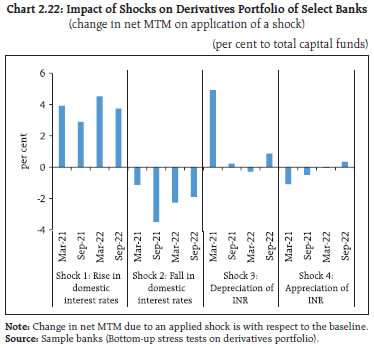
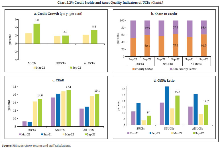
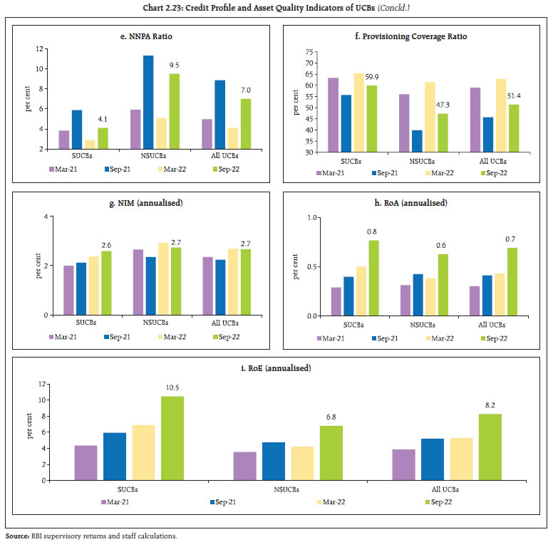 2.43 After a significant improvement in March 2022, GNPA ratios of UCBs have worsened again for both SUCBs (from 7.5 to 9.1 per cent) and NSUCBs (from 11.6 to 15.8 per cent) in September 2022. Their NNPA ratios have also deteriorated in H1:2022-23 (Charts 2.23 d and e). Despite increase in provisions, there was a decline in PCR of NSUCBs and SUCBs to 47.3 per cent and 59.9 per cent, respectively (Chart 2.23 f). The concomitant rise in CRAR and decline in PCR indicate lower provisioning relative to GNPA. Going forward, in the absence of improving profitability, additional provisioning to meet increase in NPAs would result in reduction of capital levels. 2.44 While net interest margin (NIM) remained steady in September 2022, profitability in terms of RoA and RoE ratios has improved continuously since March 2021 (Chart 2.23 g, h and i). II.2.1 Stress Testing 2.45 Stress tests have been conducted on a select set of UCBs30 to assess credit risk (default risk and concentration risk), market risk (interest rate risk in trading book and banking book) and liquidity risk, based on their reported financial positions as of September 2022. 2.46 The results show that (a) in all the five parameters tested, a few banks failed even in the baseline scenario; (b) impact of credit default risk is higher than credit concentration risk in all three scenarios; (c) impact of shock on trading book is minimal; (d) severe stress on banking book would cause failure of a large number of UCBs and (e) liquidity shocks impact the largest number of UCBs (Chart 2.24). Under the severe stress scenario, system level CRAR diminishes by 349 bps, 337 bps and 90 bps for credit default risk, credit concentration risk and interest rate risk in trading book, respectively; while NII declines by around 20 per cent under the severe stress scenario for interest rate risk in banking book. II.3 Non-Banking Financial Companies (NBFCs)31 2.47 Credit extended by NBFCs is picking up momentum, with the aggregate outstanding amount at ₹31.5 lakh crore as of September 2022. Loans to the services sector (share in outstanding credit being 14.7 per cent) and personal loans (share 29.5 per cent) recorded a healthy growth rate. Industry, the largest segment of the credit portfolio (share 37.5 per cent) saw a muted growth in Q2:2022-23 with Government owned NBFCs recording moderation (Chart 2.25). 2.48 The GNPA ratio of NBFCs eased from the peak of 7.2 per cent recorded during the second wave of the pandemic to reach 5.9 per cent in September 2022, close to the pre-pandemic level. Although this softening was observed across sectors, the GNPA ratio of services sector remains in double digits (Chart 2.26). The aggregate NNPA ratio of NBFCs ebbed by 60 bps during H1:2022-23 to 3.2 per cent in September 2022 (Chart 2.27).
2.49 The capital position of NBFCs remained robust, with CRAR of 27.4 per cent as at end-September 2022. The decline of 20 bps from March 2022 was largely on account of increase in RWA as lending picked up. The return on assets (RoA) has recouped over successive half-years (Chart 2.28). 2.50 Borrowings constituted the largest source of funds for NBFCs, although their share has come down since March 2020 (Table 2.9). Their dependence on banks for funds had grown during H1:2022-23. Borrowing from banks (mostly term loans) constituted the major part of funding from banks.
| Table 2.9: NBFCs’ Sources of Funds | | (per cent) | | Item Description | Mar-20 | Sep-20 | Mar-21 | Sep-21 | Mar-22 | Sep-22 | | 1. Share Capital, Reserves and Surplus | 24.2 | 24.4 | 26.4 | 28.9 | 28.7 | 28.5 | | 2. Total Borrowings | 66.4 | 65.3 | 63.4 | 60.6 | 61.3 | 61.0 | | Of which: | | | | | | | | 2(i) Borrowing from banks | 20.3 | 19.7 | 19.9 | 18.5 | 20.5 | 21.3 | | 2(ii) CPs subscribed by banks | 0.5 | 0.5 | 0.4 | 0.3 | 0.4 | 0.7 | | 2(iii) Debentures subscribed by banks | 2.5 | 3.0 | 3.0 | 2.9 | 2.8 | 3.1 | | Total from banks [2(i)+2(ii)+2(iii)] | 23.2 | 23.2 | 23.3 | 21.7 | 23.7 | 25.1 | | 3. Others | 9.3 | 10.3 | 10.2 | 10.5 | 10.0 | 10.5 | | Total | 100.0 | 100.0 | 100.0 | 100.0 | 100.0 | 100.0 | | Source: RBI supervisory returns and staff calculations. | 2.51 The Scale Based Regulation (SBR) introduced for NBFCs classifies them into four layers namely Base Layer (NBFC-BL), Middle Layer (NBFC-ML), Upper Layer (NBFC-UL) and Top Layer (NBFC-TL) based on their size, activity, and perceived riskiness. Recently, sixteen entities have been identified for categorisation as NBFC-UL under the framework. It is observed that the NBFC-UL group recorded higher credit growth (y-o-y) of 17.2 per cent and better GNPA ratio of 4.2 per cent as of September 2022 than the overall NBFC sector. II.3.1 Stress Test32 - Credit Risk 2.52 System level stress tests for assessing the resilience of NBFC sector to credit risk shocks has been conducted for a sample of 15233 NBFCs. The tests were carried out under a baseline and two stress scenarios – medium and high risk, with increase in slippage ratio by 1 SD and 2 SDs, respectively. The capital adequacy ratio of the sample NBFCs in September 2022 stood at 26.0 per cent and the GNPA ratio at 4.0 per cent. The baseline scenario is projected for one year ahead, based on assumptions of business continuing under usual conditions. 2.53 Under the baseline scenario, CRAR of nine NBFCs – comprising 4.7 per cent of total advances of the sample companies – are observed to be less than the minimum regulatory requirement of 15 per cent. Under a medium risk shock of 1 SD increase in the slippage ratio, the GNPA ratio increases to 6.9 per cent and the resultant income loss and additional provisional requirements reduce the CRAR by 58 bps relative to the baseline. Under the high-risk shock of 2 SDs, the capital adequacy ratio of the sector declines by 85 bps relative to the baseline to 22.6 per cent. The number of NBFCs that would fail to meet the minimum regulatory capital requirement of 15 per cent increases to 10 and 13 under medium and severe stress scenarios, respectively (Chart 2.29). II.3.2 Stress Test - Liquidity Risk 2.54 The resilience of the NBFC sector to liquidity shocks has been assessed by capturing the impact of a combination of assumed increase in cash outflows and decrease in cash inflows34. The baseline scenario uses the projected outflows and inflows as of September 2022. One baseline and two stress scenarios are applied – a medium risk scenario involving 5 per cent contraction in inflows and 5 per cent rise in outflows; and a high risk scenario entailing a shock of 10 per cent decline in inflows and 10 per cent surge in outflows. The results indicate that the number of NBFCs which would face negative cumulative mismatch in liquidity over the next one year in the baseline, medium and high-risk scenarios stood at 8 (representing 1.9 per cent of asset size of the sample), 26 (9.3 per cent) and 47 (24.0 per cent), respectively (Table 2.10). II.3.3 Interest Rate Risk 2.55 Interest rate risk for NBFCs35 has been analysed under Traditional Gap Analysis (TGA) to estimate Earnings at Risk (EAR). At group level, NBFCs have shown to exhibit positive impact on earnings under scenarios of increase in interest rate due to their rate sensitive assets being higher than rate sensitive liabilities. At entity level, 4 deposit-taking and 35 NDSI NBFCs are projected to have some degree of negative impact on earnings from adverse movement of interest rate. II.4 Insurance Sector 2.56 The solvency ratio of insurance companies assesses the ability of the insurer to meet its obligations towards policyholders. It is an effective indicator of financial stability of the sector - the higher the solvency ratio, the greater the ability of the insurer to meet its liabilities. As the insurance liabilities involve estimations of the future experience of contingent events, higher solvency ratio implies higher resilience of the insurer to withstand the uncertainties of the future. The Insurance Regulatory and Development Authority of India (IRDAI) has prescribed a solvency ratio of 150 per cent as the minimum threshold limit for all the insurers. 2.57 The consolidated solvency ratio for all insurers in both life and non-life sector over the past four quarters remains above the minimum threshold limit (Table 2.11). II.5 Stress Testing of Mutual Funds 2.58 In order to strengthen risk management practices, and develop a sound framework that would evaluate potential vulnerabilities on account of plausible events and provide early warning signals, the SEBI mandated all open-ended debt schemes (except overnight schemes) to conduct stress tests as per the best practice guidelines of the Association of Mutual Funds in India (AMFI). | Table 2.10: Liquidity Risk in NBFCs | | Cumulative Mismatch as a percentage of outflows over next one year | No. of NBFCs having liquidity mismatch | | Baseline | Medium | High | | Over 50 per cent | 2 (0.4) | 2 (0.4) | 2 (0.4) | | Between 20 and 50 per cent | 0 (0.0) | 2 (0.5) | 6 (1.5) | | 20 per cent and below | 6 (1.5) | 22 (8.4) | 39 (22.1) | Note: Figures in parenthesis represent percentage share in asset size of the sample.
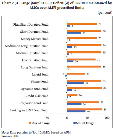
Source: RBI supervisory returns and staff calculations. | 2.59 The stress testing is being carried out by AMCs on a monthly basis for all open-ended debt schemes (except overnight schemes) to evaluate the impact of various risk parameters, viz., interest rate risk, credit risk, liquidity risk and redemption risk faced by such schemes on their net asset values (NAVs). The stress testing analysis carried out for all open-ended debt schemes (except overnight fund, gilt fund and gilt fund with 10-year constant duration) by top 10 mutual funds (based on AUM) for the months of March 2022 and September 2022 revealed no breaches of limits pertaining to these risks. | Table 2.11: Consolidated Solvency Ratio for All Insurers | | (per cent) | | Solvency Ratio as at | Life Insurance Sector | General & Health Insurance Sector | | June-22 | 200 | 180 | | March-22 | 194 | 173 | | December-21 | 189 | 172 | | September-21 | 194 | 167 | | Source: IRDAI. | 2.60 As a part of liquidity risk management for open-ended debt schemes, two types of liquidity ratios, viz., (i) Redemption at Risk (RaR) which represents likely outflows at a given confidence interval and (ii) Conditional Redemption at Risk (CRaR) which represents the behaviour of the tail at the given confidence interval, are being used. All the AMCs have been mandated to maintain these liquidity ratios (LR-RaR and LR-CRaR) above the threshold limits, which are based on the scheme type, scheme asset composition and potential outflows (modelled from investor concentration in the scheme). Mutual funds are required to carry out back testing of these liquidity ratios for all open-ended debt schemes (except overnight fund, gilt fund and gilt fund with 10-year constant duration) on a monthly basis. 2.61 The LR-RaR and LR-CRaR ratios computed by top 10 mutual funds (based on AUM) for 13 categories of open-ended debt schemes for September 2022 were well above the respective threshold limits for most of the mutual funds. However, in a few instances, the ratios were below the threshold limits, mainly on account of redemptions, which were remedied by the respective AMCs within a few days (Chart 2.30 and Chart 2.31). II.6. Stress Testing Analysis - Clearing Corporations 2.62 In order to enhance robustness of risk management framework at clearing corporations (CCs), the SEBI has issued granular norms related to core settlement guarantee fund (SGF), stress testing and default procedures. The stress testing methodology at CCs is carried out to determine the minimum required corpus (MRC) of the core SGF. 2.63 Determination of MRC of core SGF based on stress testing is carried out segment wise on a monthly basis. For determining the MRC for cash and equity derivatives segment, CCs calculate the credit exposure arising out of a presumed simultaneous default of top two clearing members (CMs). Credit exposure for each CM is determined by assessing the close-out loss arising out of closing open positions (under stress testing scenarios) and the net pay-in/pay-out requirement of the CM against the required margins and other mandatory deposits of the CM. Further, MRC of the month is determined as average of all daily worst case loss scenarios of the month and the actual MRC for any given month is determined as the higher of the MRC of the month and the MRC arrived at any time in the past. 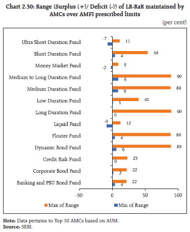
 2.64 Therefore, in line with the SEBI’s recommendation, though the monthly calculated amounts of MRC {cash as well as futures and options (F&O) segments} at a major clearing corporation based on stress testing analysis varied during the period July- October 2022 as per the change in credit exposure of CMs, the actual MRC requirement (for cash and F&O segments) remained static across the months (Table 2.12). II.7 Interconnectedness 2.65 A financial system can be visualised as a network with financial institutions as nodes and bilateral exposures as links joining these nodes. These links which could be in the form of loans to, investments in, or deposits with each other act as a source of funding, liquidity, investment and risk diversification, but could also transform in adverse conditions into channels through which shocks can spread, leading to contagion and amplification of systemic shocks. Understanding the nuances of such networks becomes critical for safeguarding macroeconomic and financial stability. | Table 2.12: Minimum Required Corpus of Core SGF Based on Stress Testing Analysis at a major Clearing Corporation | | (Amount in ₹ crore) | | Segments | July 2022 | August 2022 | September 2022 | October 2022 | | Cash Market (CM) | 172 | 148 | 149 | 155 | | Equity Derivatives Segment (FO) | 961 | 991 | 1,147 | 1,296 | | Total (CM+FO) | 1,132 | 1,139 | 1,297 | 1,451 | | Actual MRC requirement (CM+FO) | 1,558 | 1,558 | 1,558 | 1,558 | | Source: SEBI | II.7.1 Financial System Network36 37 2.66 The total outstanding bilateral exposures38 among the entities in the financial system maintained steady growth. The increase in September 2022 quarter was driven by higher borrowing requirement of SCBs and all India financial institutions (AIFIs) (Chart 2.32 a). 2.67 SCBs continued to have the largest bilateral exposures in the Indian financial system, reaching the pre-pandemic level in September 2022. The share of NBFCs and AMC-MFs declined on a y-o-y basis, while that of AIFIs increased (Chart 2.32 b). 2.68 In terms of inter-sectoral exposures39, AMC-MFs, followed by insurance companies, were the biggest fund providers in the system, whereas NBFCs and HFCs were the largest receivers of funds, followed by PVBs. Among the bank groups, PSBs, FBs and UCBs had net receivable positions vis-à-vis the entire financial sector, whereas PVBs and SFBs had net payable positions (Chart 2.33). 2.69 Net receivables of AMC-MFs and insurance companies from the financial system increased during the period September 2021 to September 2022. On the other hand, net payables of PVBs, NBFCs and HFCs increased during the period. PSBs’ role as a fund provider to the system has diminished as credit growth outpaced deposit growth for PSBs (Chart 2.34).
a. Inter-bank Market 2.70 Inter-bank exposures accounted for 3.3 per cent of the total assets of the banking system as of September 2022, with fund-based exposure constituting the major part (2.5 per cent). In absolute terms, both fund-based40 and non-fund-based exposures41 continued to increase (Chart 2.35). 2.71 PSBs remained the dominant player in the inter-bank market, though their share decreased marginally in Q2:2022-23, while the share of PVBs and FBs increased marginally in the same period (Chart 2.36). 2.72 About 74 per cent of the fund-based inter-bank market was short-term (ST) in nature in which ST deposits had the highest share, followed by ST loans and call money market exposure. Long-term (LT) loans predominated in LT fund-based inter-bank exposures (Chart 2.37).
b. Inter-bank Market: Network Structure and Connectivity 2.73 The inter-bank market typically has a core-periphery network structure42 43. As of end-September 2022, four banks were in the innermost core and seven banks in the mid-core circle. The four banks in the innermost core included one large public sector bank and three private sector banks. The banks in the mid-core were PSBs and PVBs, while most of the old PVBs along with FBs, SUCBs and SFBs formed the periphery (Chart 2.38). 2.74 The degree of interconnectedness in the banking system (SCBs), as measured by the connectivity ratio44, increased marginally from March 2022 to September 2022. However, the cluster coefficient45 declined to 41.3 per cent in September 2022 from 42.6 per cent in March 2022 (Chart 2.39). c. Exposure of AMCs-MFs 2.75 The gross receivables of AMC-MFs stood at ₹11.49 lakh crore (around 33 per cent of their average AUM) whereas their gross payables were ₹0.85 lakh crore as at end-September 2022. SCBs were the major recipients of their funding. Their receivables from AIFIs also increased, however receivables from NBFCs and HFCs declined (Chart 2.40 a). 2.76 In the asset composition of AMC-MFs, the share of equity holdings continued to increase as the equity inflow to MFs remained buoyant, while the shares of CDs and CPs maintained steady growth sequentially. Furthermore, the share of long-term (LT) debt continued to decline (Chart 2.40 b). d. Exposure of Insurance Companies 2.77 The gross receivables of insurance companies stood at ₹7.90 lakh crore and gross payables at ₹0.55 lakh crore in September 2022. SCBs were the largest recipients of their funds, followed by NBFCs and HFCs. More than 90 per cent of their assets were in the form of LT debt and equity (Chart 2.41 a and b).
e. Exposure to NBFCs 2.78 NBFCs were the largest net borrowers of funds from the financial system, with gross payables of ₹13.22 lakh crore and gross receivables of ₹1.93 lakh crore as at end-September 2022. Over half of their borrowings were from SCBs and this share remained stable during Q2:2022-23 as their reliance on funding from AMC-MFs continued to reduce (Chart 2.42 a). Instrument wise, the NBFC funding mix saw a marginal rise in LT loans and LT debt instruments whereas the share of CPs declined during Q2:2022-23 (Chart 2.42 b). f. Exposure to HFCs 2.79 HFCs were the second largest net borrowers of funds from the financial system, with gross payables of ₹7.70 lakh crore and gross receivables of ₹0.57 lakh crore as at end-September 2022. As in the case of NBFCs, the reliance of HFCs on funding from SCBs has been high; however it declined marginally during the quarter. Their share of borrowings from AMC-MFs is on a declining trend while the share of insurance companies increased significantly in September quarter (Chart 2.43 a). The proportion of resource mobilisation through LT loans maintained steady growth sequentially. The share of funds mobilised through LT debt instruments and CPs varied through the year (Chart 2.43 b).
g. Exposure of AIFIs 2.80 AIFIs were net borrowers of funds from the financial system with their gross payables and gross receivables having increased to ₹5.91 lakh crore and ₹5.47 lakh crore, respectively, in September 2022. They raised funds mainly from SCBs (primarily PVBs), AMC-MFs and insurance companies (Chart 2.44 a). Given their nature of operations, LT Loans, LT debt and LT deposits remained their preferred instruments for raising funds, but the combined share of these instruments has declined to 59.7 per cent from 68.7 per cent a year ago, and their mobilisation of funds through CPs increased in Q2:2022-23 (Chart 2.44 b). II.7.2 Contagion Analysis 2.81 Contagion analysis uses network technology to estimate the systemic importance of individual banks. The failure of a systemically important bank leads to solvency and liquidity losses for the banking system. The scale of losses depends on the capital and liquidity positions of banks as well as the extent and nature of exposure (whether it is a lender or a borrower) and magnitude of the interconnections that the failing bank has with the rest of the banking system. a. Joint Solvency46-Liquidity47 Contagion Losses for SCBs due to Bank Failure 2.82 A contagion analysis of the banking network based on end-September 2022 position indicates that if the bank with the maximum capacity to cause contagion losses fails, it will cause a solvency loss of 2.49 per cent (as compared with 2.83 per cent in March 2022) of total Tier 1 capital of SCBs and a liquidity loss of 0.31 per cent (0.02 per cent in March 2022) of total HQLA of the banking system. The analysis also shows that contagion losses due to failure of the five banks with the maximum capacity to cause contagion losses would not lead to the failure of any additional bank (Table 2.13). b. Solvency Contagion losses for SCBs due to NBFC/HFC Failure 2.83 The failure of any NBFC or HFC would also act as a solvency shock to their lenders depending on the extent of exposure, and solvency losses can spread through contagion. 2.84 By end-September 2022, the idiosyncratic failure of an NBFC with the maximum capacity to cause solvency losses to the banking system would have impacted bank’s total Tier 1 capital by 2.63 per cent (as compared with 2.40 per cent in March 2022). In a similar scenario of an HFC failure, the impact on total Tier 1 capital would be 5.90 per cent (5.88 per cent in March 2022). In both cases, however, it would not lead to failure of any bank (Tables 2.14 and 2.15). | Table 2.13: Contagion Losses due to Bank Failure – September 2022 | | Trigger Code | % of Tier 1 capital of the Banking System | % of HQLA | Number of Bank defaulting due to Solvency | Number of Bank defaulting due to Liquidity | | Bank 1 | 2.49 | 0.31 | 0 | 0 | | Bank 2 | 2.18 | 0.09 | 0 | 0 | | Bank 3 | 2.11 | 0.07 | 0 | 0 | | Bank 4 | 2.04 | 0.01 | 0 | 0 | | Bank 5 | 2.00 | 0.02 | 0 | 0 | Note: ‘Trigger banks’ have been selected on the basis of solvency losses caused to the banking system.
Source: RBI supervisory returns and staff calculations. |
| Table 2.14: Contagion Losses due to NBFC Failure – September 2022 | | Trigger Code | Solvency Losses as % of Tier 1 Capital of the Banking System | Number of Banks Defaulting due to solvency | | NBFC 1 | 2.63 | 0 | | NBFC 2 | 2.33 | 0 | | NBFC 3 | 1.83 | 0 | | NBFC 4 | 1.79 | 0 | | NBFC 5 | 1.54 | 0 | Note: Top five ‘Trigger NBFCs’ have been selected on the basis of solvency losses caused to the banking system.
Source: RBI supervisory returns and staff calculations. |
| Table 2.15: Contagion Losses due to HFC Failure – September 2022 | | Trigger Code | Solvency Losses as % of Tier 1 Capital of the Banking System | Number of Banks Defaulting due to solvency | | HFC 1 | 5.90 | 0 | | HFC 2 | 4.70 | 0 | | HFC 3 | 1.74 | 0 | | HFC 4 | 1.74 | 0 | | HFC 5 | 1.14 | 0 | Note: Top five ‘Trigger HFCs’ have been selected on the basis of solvency losses caused to the banking system.
Source: RBI supervisory returns and staff calculations. | c. Solvency Contagion Impact48 after Macroeconomic Shocks to SCBs 2.85 The contagion from the failure of a bank is likely to get magnified if macroeconomic shocks result in distress to the banking system. In such a situation, similar shocks may cause some SCBs to fail the solvency criterion, which then acts as a trigger for further solvency losses. 2.86 In the previous iteration, the shock was applied to the entity that could cause the maximum solvency contagion losses. In another iteration in which the initial impact of such a shock on an individual bank’s capital is taken from the macro-stress tests49, the initial capital loss due to macroeconomic shocks stood at 5.64 per cent, 10.98 per cent and 16.67 per cent of Tier I capital for baseline, medium and severe stress scenarios, respectively. No bank fails to maintain Tier I capital adequacy ratio of 7 per cent in any of the scenarios. As a result, there are no additional solvency losses to the banking system due to contagion (over and above the initial loss of capital due to the macro shocks) (Chart 2.45). Summary and Outlook 2.87 Keeping pace with the underlying momentum of domestic economic activity, financial sector entities have engaged in active intermediation to support the demand for funds. Lending has moved to a higher trajectory and has become broad based. Capital positions remain strong. The asset quality of banks and NBFCs has improved further, but some deterioration is evident for UCBs. Macro stress tests indicate that SCBs can withstand moderate to severe adverse macroeconomic circumstances without significant capital impairment. 2.88 Sensitivity analysis shows that PVBs and FBs would face lower erosion in CRAR than PSBs, if credit risk materialises, and credit concentration risk may not be substantial. Network analysis results suggest that contagion losses have declined marginally during H1:2022-23. In the case of macroeconomic shocks, there are no additional solvency losses to the banking system due to contagion.
|