|
Inflation forecasts are critical for the conduct of a forward-looking monetary policy and play a special role in an inflation-targeting framework by acting as an intermediate target. The analysis in this paper suggests that the episodes of large inflation forecasts errors for India were associated with large and unanticipated shocks emanating from prices of food items, especially perishables such as vegetables. Cross-country evidence suggests that there is a positive correlation of forecast errors with the share of food items in the Consumer Price Index (CPI) basket. Forecasts by the Reserve Bank of India staff generally satisfy the key properties of unbiasedness and efficiency and compare well with those of select central banks.
I. Introduction
Monetary policy operates with long and variable lags, i.e., the action taken today will impact the ultimate objectives of monetary policy of growth and price stability only after a few quarters. For this reason, monetary policy needs to be forward-looking. In this context, inflation forecasts, by acting as an intermediate target, play a special role in an inflation-targeting framework. If the medium-term inflation forecasts are above (or, below) the inflation target, they signal the need for a monetary tightening (or, easing) to bring inflation back to target level. Hence, consistently reliable forecasts of inflation facilitate a sustained attainment of desired policy goals; conversely, large and persistent inflation forecast errors can lead to sub-optimal conduct of monetary policy and outcomes.
The amended Reserve Bank of India Act, 1934, which came into effect in June 2016, paved the way for a flexible inflation targeting (FIT) framework in India by specifying the primary objective of monetary policy as maintaining price stability while keeping in mind the objective of growth. To operationalise this mandate, the Government of India notified a medium-term inflation target of 4 per cent, with a band of +/- 2 per cent for the period from August 2016 to March 2021. The inflation target has been fixed in terms of all-India CPI-Combined published by the Central Statistics Office (CSO).
The bi-monthly resolutions of the Monetary Policy Committee (MPC) provide inflation forecasts for up to four quarters ahead. The Monetary Policy Report (MPR), released twice in a year (April and October), provides inflation forecasts for up to eight quarters ahead. Inflation forecasts were also an integral part of monetary policy communication even before the adoption of the FIT framework in 2016, but they assumed a special significance under the FIT regime.
Against this backdrop, this paper analyses the forecast performance based on the all India CPI, with a special focus on identifying the episodes of large forecast errors and explaining the underlying factors. The study also undertakes a formal evaluation of the performance of forecasts of inflation based on key properties such as accuracy, efficiency, unbiasedness and autocorrelation for the period April 2015 to September 2018 in a cross-country perspective.2
The paper is organised as follows. Section II sets out a brief overview of the process of inflation projections at the RBI. Section III sets out the stylised facts relating to the inflation behaviour and assesses the short-term forecasting performance. Section IV undertakes a detailed analysis of RBI staff’s inflation forecasting marksmanship in a cross-country perspective. Section V concludes the paper.
II. The Process of Staff Forecasting
The inflation forecasting framework at the Reserve Bank is highly detailed and rigorous based on three mutually consistent and reinforcing pillars. These are (i) nowcasts for the first month or the most recent projections, (ii) short-term (4-quarter ahead) projections and (iii) medium-term (2-year ahead) projections. Nowcasts feed into short-term projections as initial conditions and the short-term projections, in turn, feed into medium term projections as their initial conditions (Chart 1).
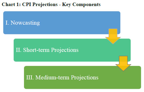 Nowcasting for CPI inflation is arrived at using high frequency/daily data available from secondary sources as well as using the in-house surveys conducted by the Reserve Bank. The focus of nowcasts is primarily on estimating near-term food inflation using retail as well as mandi prices and arrivals data. Short-run projections are based on a full information projection system that employs competing models (structural time-series analysis; multivariate regression analysis; forward looking surveys and lead indicators) aggregated parsimoniously through root mean squared error (RMSE) scores3. The baseline short-term projections then feed into the macro-economic models for medium term projections, build to capture key India-specific features of inflation and monetary policy transmission. The workhorse macro-model used in the RBI for medium-term projections is a forecasting and policy analysis system (FPAS) based quarterly projection model (QPM), which provides a consistent framework for conducting simulations and counterfactual experiments (Benes et al, 2016).
III. Inflation Forecast by the RBI Staff – An Assessment
Stylised Facts
Before going into a discussion of the inflation performance, this section presents key stylised facts of the inflation process since 2012 to place the overall discussion on inflation projection performance in proper perspective.
The inflation process in India has gone through a sharp disinflation phase since 2014. This has been marked by a sustained fall in the contribution of food inflation4 to overall inflation – from close to 60 per cent in 2013-14 to about 7 per cent in 2018-19 (up to December 2018) (Chart 2).
As food inflation moderated, there was also a shift in its drivers. Elevated inflation during 2012-13 to 2013-14 reflected the combined impact of high inflation in cereals, pulses, egg, fish and meat, milk and vegetables. However, inflation in all these categories declined sharply, with pulses even moving into deflation beginning 2017, pulling down food inflation to around 1 per cent in 2018-19 (Chart 3).
Another noteworthy feature was volatile movements in vegetables inflation throughout. Volatility in vegetables prices translated almost one-on-one to overall food inflation, given the magnitude of price variations and large weight of vegetables in CPI - Food (Chart 4).
The correlation between the monthly changes in overall food inflation and vegetables is as high as 0.9. The correlation of other food items with overall food group is low. There were only two other items with significant correlation, though with much lower magnitudes, with the changes in overall food inflation, i.e., fruits (0.4) and oils (0.3). Vegetables price movements, thus, had a major role in explaining in the month to month variations in food inflation (Table 1).
Table 1: Correlation Coefficient of the Changes in Food Groups Inflation
with Changes in Overall CPI Food Inflation (2012-18) |
| CPI Food Sub-groups |
Correlation Coefficient with CPI Food |
| CPI Vegetables |
0.9* |
| CPI Fruits |
0.4* |
| CPI Oils |
0.3* |
| CPI Cereals |
0.2 |
| CPI Egg |
0.2 |
| CPI Pulses |
0.2 |
| CPI Sugar |
0.2 |
| CPI Prepared Meals |
0.2 |
| CPI Meat |
0.1 |
| CPI Non-alcoholic Beverages |
0.1 |
| CPI Milk |
0.0 |
| CPI Spices |
-0.1 |
* Significant at 1% level.
Source: CSO; authors’ estimates. |
Among non-food CPI, large volatility was also observed in global crude oil prices with attendant implications for its pass-through to domestic petroleum product prices and inflation (Charts 5 and 6).
Sources of Short-term Forecast Errors
The stylised facts as outlined above point to high volatility in the behaviour of food and oil, which had a significant bearing on the overall inflation outcomes in relation to projections.
An examination of the actual CPI inflation outcomes for the period April 2015 to December 2018 indicates two episodes - Q3 and Q4:2016-17 and Q2:2018-19 - when actual inflation outcomes deviated significantly from the 1-quarter ahead projections. These were periods of large and unanticipated shocks originating primarily from food (Chart 7).
Q3 and Q4: 2016-17 – Collapse in Vegetable and Pulses Prices
The prices of vegetables rose sharply during April-June 2016, reflecting a strong seasonal uptick in prices of tomatoes but thereafter moderated and stabilised by October 2016. However, following the shock of demonetisation, there was a sudden, large and broad-based collapse in vegetable prices (Chart 8).
Another factor was a sharp decline in pulses prices (Chart 9). Between January 2015 to July 2016, pulses prices rose by around 50 per cent. However, they started to moderate in Q3:2016-17 and declined sharply further by as much as 20 per cent by Q4 from the July peak. A combination of factors contributed to this dramatic turnaround - such as record production in 2016-17, resulting from adequate rainfall and better area coverage after two consecutive years of production shortfall, favourable supply side measures taken by the government such as imports at zero import duty, extension in stock limit of pulses, higher MSPs and maintaining buffer stocks. This sharp pace of decline was in a sharp contrast to historical trends.
As a result of a sharp decline in vegetables and pulses prices, overall food prices declined sequentially month-on-month (Chart 10). This pushed food group into deflation by May 2017 in contrast to the high inflation rate of 8.0 per cent in the food group in July 2016.
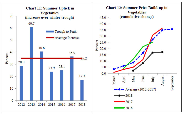
Q2:2018-19 – Unusually Muted Summer Pick up in Vegetable Prices
Vegetables prices normally pick up in summer months (March to July) with an accentuation of pace during June-July, coming from relatively lower supply in mandis during these months. However, during Q2: 2018-19, the trough to peak seasonal summer uptick in prices in 2018 was the lowest since the release of the all India CPI series (Chart 11). Secondly, the build-up in prices was also unusual – first delayed to May (normally it starts in March-April) and thereafter plateaued by July (in the past, vegetable prices used to pick up sharply during this period) (Chart 12). The tepid rise in vegetable prices during summer months and lack of any pick up thereafter led to an unusual and negative build up in food prices between July-December (Chart 10).
 To sum up, large projection errors that occurred in recent years can be attributed to the unexpected sharp fall in food inflation. However, it also needs to be assessed as to how inflation forecasts have fared in general in terms of key properties such as accuracy, unbiasedness, efficiency, and autocorrelation (lack of co-movement with the past errors) in a cross-country perspective. This is the subject matter of next section.
IV. Analysis of Forecast Performance and a Cross Country Comparison
For studying the forecast performance, the bi-monthly policy projections have been used for the period April 2015-September 2018. Within this period, inflation in India, as discussed in the previous section, eased significantly for a few months following demonetisation in November 2016, which imparted a large bias to the forecasts made prior to November 2016 and for a few subsequent months. The analysis, therefore, presents results for the full sample period as well as for the period excluding demonetisation5. The sample period for India also includes the time of introduction of goods and services tax – a major structural reform measure – in July 2017 which, as the cross-country evidence suggests, adds uncertainty to the inflation outlook during the implementation stage (RBI, 2016). Indeed, inflation excluding food and fuel eased significantly in the quarter April-June 2017, pending price revisions ahead of GST implementation, which imparted another downward bias to the projections.
In the empirical assessment below, we look at the forecasting performance for various horizons (one-, two-, three- and four-quarter ahead forecasts). For the cross-county analysis, we focus on some of the major central banks for which data on inflation forecasts are available in the public domain at a quarterly frequency for various forecast horizons for April 2015 onwards. This criterion resulted in the inclusion of six countries, including both advanced and emerging economies – Sweden, the UK, Czech Republic, Hungary, New Zealand and South Africa – in the sample.
Some major central banks such as the US Federal Reserve, the European Central Bank, Bank of Japan and the Reserve Bank of Australia could not be included in the forecast evaluation analysis for different reasons. The US Federal Open Market Committee provides inflation forecasts only for the quarter ended December of each year (and not for all the four quarters of the year). In the case of ECB, data are publicly available only for the period from June 2017 onwards. The Bank of Japan’s forecasts are available only on a calendar year basis and not on a quarterly basis. The Reserve Bank of Australia’s forecasts are available only for June and December of every year.
Three critical aspects need to be noted while assessing cross-country forecast performance. First, target inflation rates as well as the actual average inflation rates differ across countries. The CPI inflation target for India is 4 per cent, while the targets are 2 per cent each for the UK, Sweden, Czech Republic and New Zealand. For Hungary and South Africa, the targets are 3 per cent and 4.5 per cent, respectively. Actual inflation over the sample period of this study (April 2015-September 2018) averaged 4.3 per cent for India for the full sample and 4.7 per cent for the sample excluding October 2016-June 2017. For the other countries included in the sample, the inflation averaged 1.1 per cent for New Zealand, 1.4 per cent for Hungary, 1.5 per cent each for Czech Republic and UK, 1.6 per cent for Sweden and 5.3 per cent for South Africa. In view of these large differences across the sample countries, we also look at standardised errors (i.e., errors divided by the actual average inflation rates). Standardisation, with respect to inflation target and/or actual inflation, provides a measure of relative errors (akin to coefficient of variation that measures relative variability). Such standardisation makes cross country evaluation comparable.
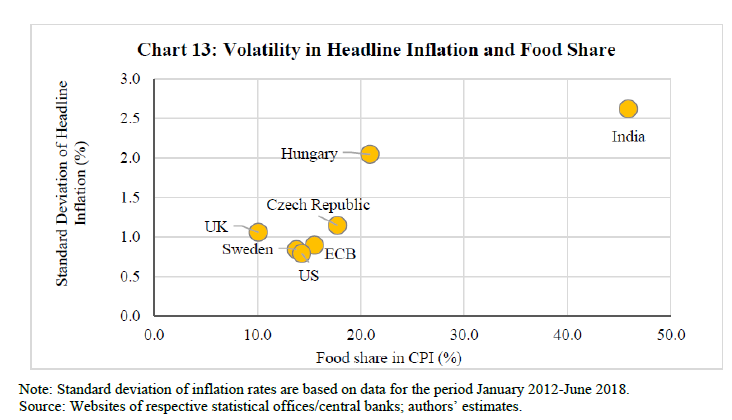
Second, the composition of consumption basket varies significantly across countries. The share of food in CPI in India (45.9 per cent) is much higher than the 10-20 per cent in other countries. Along with higher share of food items, sharp movements in prices (as detailed in the previous section for India) due to large exogenous supply side shocks can impart sizable volatility to headline inflation (Chart 13). An analysis across select countries shows a high correlation of around 0.9 between the share of food in CPI and the volatility in headline inflation. Thus, large share of food items along with the associated high food price volatility can be challenging for inflation forecasting.
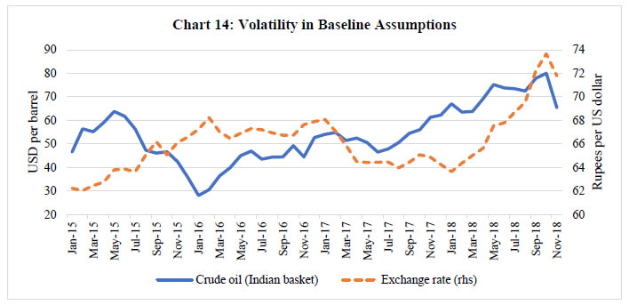
 Third, two key assumptions at the time of making projections are about crude oil and the exchange rate. Sharp volatility has been observed in the actual dynamics of these key baseline variables (Chart 14). This volatility in the path of the conditioning variables can impart bias, particularly at the longer end, and persistence in the forecast errors.
 Against this backdrop, this Section undertakes a formal evaluation of the forecast performance in terms of major parameters: accuracy, unbiasedness, efficiency, and autocorrelation. ‘Unbiasedness’ test assesses as to whether there is any systematic bias (upward/downward) in the forecasts. ‘Efficiency’ test attempts to examine as to whether all the available information has been used while making the forecasts (Bank of England, 2015; Gestsson, 2018). ‘Autocorrelation’ test is used to test correlation in forecast errors over time (for example, whether higher forecast errors today also lead to higher errors tomorrow). RBI staff forecasts are also evaluated against the benchmark random walk model.
Accuracy
Accuracy of forecasts could be analysed through examination of forecast errors (defined as actual inflation outcome minus the forecast). Mean error (ME), mean absolute error (MAE) and root mean squared error (RMSE) are three frequently used measures for comparing forecast performances (Table 2). MAE and RMSE provide an assessment of the absolute size of errors, without letting different signs of errors cancelling out. However, while these measures assess the quantum of error, they ignore their direction. Mean error (ME), in contrast, gives a measure of direction of average error in relation to the actual inflation outcomes. Given the earlier noted differences in inflation rates and targets across the sample countries, we also analyse standardised errors (i.e., errors in relation to the average inflation over the sample period).
Table 2: Measures for Assessing Accuracy of Forecasts  with Actual Inflation (π) with Actual Inflation (π) |
| Mean errors (ME): This is the average deviation of actual inflation readings from their projections. It is measured as under: |
|
| Mean absolute errors (MAE): This is the average of absolute deviation of actual inflation from its forecast, computed as under: |
|
| Root mean squared error (RMSE): This measure is a frequently used measure of the differences between observed values and those predicted or estimated. It is defined as under: |
|
| Standardisation: For making meaningful cross-country comparisons, the above three measures have also been standardised with respect to the average inflation of all countries. |
For India, we report results for the full sample as well as for the sample excluding the demonetisation quarter and the subsequent two quarters (i.e., excluding the forecasts for the period October 2016-June 2017). We focus on the sample excluding demonetisation in the subsequent analysis, given the large unanticipated nature of the shock.
Results of the various forecast error measures for India and the other sample countries are presented in Table 3. The mean error (average across all the four horizons) for RBI staff estimates for the sample excluding the demonetisation period is (-) 30 basis points (bps)6, compared to a range of 0 to (-) 40 bps for the other sample countries (Table 3, panel a).7 The issue as to whether these errors are statistically significant will be addressed later in this section. The standardised mean error is around 7 per cent for India vis-à-vis 0-26 per cent for the other sample countries (Table 3, panel b).
The mean absolute error (averaged across all the four forecast horizons) and the corresponding standardised error for RBI staff estimates is 40 bps (20-60 bps for other countries) and 9 per cent (10-41 per cent for other countries, respectively) (Table 3, panel c and d). Finally, the RMSE for Indian forecasts averaged 60 bps, compared to 30-80 bps for the other sample countries. However, the standardised RMSE for India at 12 per cent was lower than that of most other countries (11-57 per cent) (Table 3, panel e and f). One key caveat of the analysis is the relatively short sample period. For some of the sample countries for which longer time series data are available, forecast errors are higher than reported in this study.8
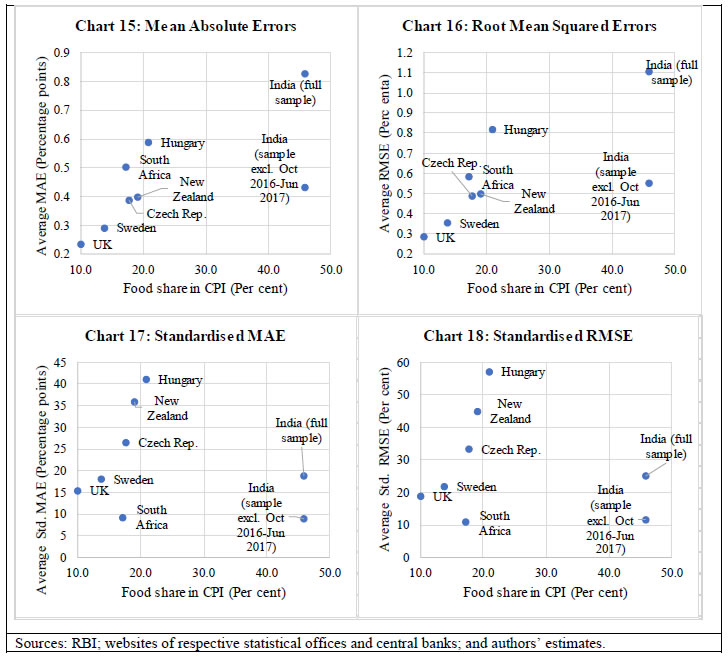
The previous section discussed the role of food share and its volatility in forecast errors. A cross-country analysis of forecast errors and food share shows that India stands out with a very large share of food in CPI and relatively high forecast errors (Chart 15 and 16). However, after the forecast errors are standardised with respect to average observed inflation – to get a measure that corrects for difference in inflation values and provides a measure of comparable errors as discussed earlier – there is a flattening of relationship between the forecast errors and the share of food group. For India, the standardised forecast errors are lower than in some sample countries (Charts 17 and 18).
| Table 3: Forecast Errors |
| Item |
India (full sample) |
India (sample excl. forecasts for Oct 2016-Jun 2017) |
UK |
Czech Republic |
Sweden |
Hungary |
New Zealand |
South Africa |
| a. Mean Error (Percentage points) |
|
|
|
|
|
|
|
| 1-quarter ahead error |
-0.3 |
-0.1 |
0.0 |
0.1 |
0.0 |
-0.2 |
0.1 |
-0.2 |
| 2-quarter ahead error |
-0.6 |
-0.3 |
0.0 |
0.1 |
0.0 |
-0.3 |
0.0 |
-0.4 |
| 3-quarter ahead error |
-0.9 |
-0.3 |
0.0 |
0.0 |
0.0 |
-0.5 |
-0.1 |
-0.5 |
| 4-quarter ahead error |
-1.1 |
-0.5 |
0.0 |
-0.1 |
0.0 |
-0.6 |
-0.1 |
-0.6 |
| Average |
-0.7 |
-0.3 |
0.0 |
0.0 |
0.0 |
-0.4 |
0.0 |
-0.4 |
| b. Standardised Mean Error (Per cent) |
|
|
|
|
|
|
| 1-quarter ahead error |
-6.8 |
-2.3 |
-1.6 |
5.1 |
-0.9 |
-10.7 |
5.8 |
-4.5 |
| 2-quarter ahead error |
-14.8 |
-7.4 |
-0.4 |
6.3 |
1.4 |
-19.0 |
-2.3 |
-8.0 |
| 3-quarter ahead error |
-20.3 |
-5.7 |
-1.1 |
-2.4 |
2.7 |
-34.1 |
-9.8 |
-9.9 |
| 4-quarter ahead error |
-25.9 |
-11.0 |
2.0 |
-6.0 |
-0.1 |
-41.9 |
-11.4 |
-10.4 |
| Average |
-17.0 |
-6.6 |
-0.3 |
0.7 |
0.8 |
-26.4 |
-4.4 |
-8.2 |
| c. Mean Absolute Error (Percentage points) |
|
|
|
|
|
|
| 1-quarter ahead error |
0.4 |
0.3 |
0.1 |
0.3 |
0.2 |
0.3 |
0.2 |
0.3 |
| 2-quarter ahead error |
0.7 |
0.4 |
0.2 |
0.5 |
0.3 |
0.5 |
0.3 |
0.5 |
| 3-quarter ahead error |
1.0 |
0.4 |
0.3 |
0.4 |
0.4 |
0.7 |
0.5 |
0.6 |
| 4-quarter ahead error |
1.1 |
0.5 |
0.4 |
0.4 |
0.4 |
0.9 |
0.5 |
0.6 |
| Average |
0.8 |
0.4 |
0.2 |
0.4 |
0.3 |
0.6 |
0.4 |
0.5 |
| d. Standardised Mean Absolute Error (Per cent) |
|
|
|
|
|
|
| 1-quarter ahead error |
10.3 |
6.3 |
4.0 |
20.0 |
9.4 |
23.6 |
20.7 |
5.9 |
| 2-quarter ahead error |
16.8 |
9.6 |
12.4 |
31.6 |
15.8 |
31.9 |
31.0 |
8.8 |
| 3-quarter ahead error |
22.7 |
9.3 |
18.3 |
26.4 |
22.5 |
49.1 |
43.2 |
11.8 |
| 4-quarter ahead error |
26.4 |
11.7 |
27.6 |
28.5 |
25.1 |
60.1 |
49.3 |
11.3 |
| Average |
19.0 |
9.2 |
15.6 |
26.6 |
18.2 |
41.2 |
36.1 |
9.5 |
| e. Root Mean Squared Error (RMSE) (Percentage points) |
|
|
|
|
|
| 1-quarter ahead error |
0.6 |
0.4 |
0.1 |
0.3 |
0.2 |
0.5 |
0.3 |
0.4 |
| 2-quarter ahead error |
1.0 |
0.6 |
0.2 |
0.5 |
0.3 |
0.7 |
0.4 |
0.5 |
| 3-quarter ahead error |
1.3 |
0.6 |
0.3 |
0.5 |
0.4 |
1.0 |
0.6 |
0.7 |
| 4-quarter ahead error |
1.5 |
0.7 |
0.5 |
0.6 |
0.5 |
1.1 |
0.7 |
0.7 |
| Average |
1.1 |
0.6 |
0.3 |
0.5 |
0.4 |
0.8 |
0.5 |
0.6 |
| f. Standardised RMSE (Per cent) |
|
|
|
|
|
|
|
| 1-quarter ahead error |
14.5 |
7.6 |
5.6 |
23.2 |
11.7 |
32.2 |
26.1 |
7.0 |
| 2-quarter ahead error |
22.9 |
13.5 |
13.9 |
37.4 |
19.6 |
47.1 |
37.8 |
10.2 |
| 3-quarter ahead error |
30.6 |
11.9 |
21.7 |
35.3 |
26.8 |
69.3 |
54.1 |
13.3 |
| 4-quarter ahead error |
33.5 |
14.3 |
34.8 |
38.1 |
29.9 |
80.4 |
62.7 |
13.3 |
| Average |
25.4 |
11.8 |
19.0 |
33.5 |
22.0 |
57.3 |
45.2 |
11.0 |
Note: Forecast error is defined as actual inflation minus the forecast. Standardised measures are errors divided by the respective country’s average inflation over the sample period.
Source: RBI; websites of respective central banks/statistical offices; and authors’ estimates. |
 Unbiasedness
For a forecast to be unbiased, a necessary and sufficient condition is that the average error should be zero. Unbiasedness is generally considered as an important attribute of forecasts as it implies that forecasts are identical to outturns on average. It is also a necessary condition for efficiency of forecasts (Freedman, 2014). Unbiasedness can be tested by regressing forecast errors on a constant, i.e., by estimating the following equation:
where et+q,t is forecast error q quarters ahead, αq is constant, and ut+q,t is the residual term. If the forecast is unbiased, then in the above equation E(et+q,t) = 0, i.e., the estimate of the constant term (αq) should be statistically insignificant. If the estimate of αq < 0 (and statistically significant), it implies that the forecasts are biased upwards (i.e., the forecasts exceed the actual outturns) and vice versa for αq > 0 (downward bias in the forecasts).
The results of unbiasedness test for one, two, three and four quarter ahead forecasts are presented in Table 4. For India, for the full sample period, there is evidence of a statistically significant upward bias, reflecting an unanticipated decline in inflation for a few months after November 2016. However, excluding the period of demonetisation, the forecasts for one and three quarters ahead are unbiased, while there is an evidence of bias for two- and four-quarter ahead forecasts; the relatively limited sample size, especially for three- and four-quarter ahead forecast horizons constrains a conclusive assessment. The hypothesis of unbiased forecasts cannot be rejected for most other countries in the sample, other than for South Africa.
| Table 4: Unbiasedness Test |
| (Estimate of αq in equation (1), i.e., et = αq + ut) |
| Forecast horizon |
India (full sample) |
India (sample excl. forecasts for Oct 2016-Jun 2017) |
Czech Republic |
Hungary |
Sweden |
UK |
New Zealand |
South Africa |
| 1 quarter ahead |
-0.30** |
-0.11 |
0.07 |
-0.15 |
-0.01 |
-0.02 |
0.10 |
-0.24*** |
| |
(0.03) |
(0.24) |
(0.43) |
(0.24) |
(0.74) |
(0.36) |
(0.26) |
(0.00) |
| |
[20] |
[16] |
[14] |
[13] |
[20] |
[14] |
[14] |
[21] |
| 2 quarter ahead |
-0.64*** |
-0.34** |
0.09 |
-0.27 |
0.02 |
-0.01 |
0.00 |
-0.42*** |
| |
(0.00) |
(0.03) |
(0.57) |
(0.17) |
(0.76) |
(0.93) |
(1.00) |
(0.00) |
| |
[19] |
[15] |
[13] |
[12] |
[19] |
[13] |
[13] |
[20] |
| 3 quarter ahead |
-0.88*** |
-0.27 |
-0.03 |
-0.49 |
0.04 |
-0.02 |
-0.07 |
-0.53*** |
| |
(0.00) |
(0.11) |
(0.83) |
(0.10) |
(0.68) |
(0.87) |
(0.68) |
(0.00) |
| |
[17] |
[11] |
[12] |
[11] |
[18] |
[12] |
[12] |
[18] |
| 4 quarter ahead |
-1.13*** |
-0.51*** |
-0.09 |
-0.60 |
-0.00 |
0.03 |
-0.14 |
-0.55*** |
| |
(0.00) |
(0.01) |
(0.63) |
(0.10) |
(0.99) |
(0.86) |
(0.51) |
(0.00) |
| |
[15] |
[9] |
[11] |
[10] |
[16] |
[11] |
[11] |
[17] |
Notes: Figures in parentheses are p-values.
Figures in square brackets are number of observations.
***,**,*: Significant at <1%, <5% and <10% levels, respectively.
Source: Authors’ estimates. |
Efficiency
An efficient forecast makes use of all the available information at the time of the forecast, which would imply no correlation of forecast errors with the available information. One crucial piece of such information is the actual inflation rate at the time of the forecast and the efficiency of forecasts can be assessed by estimating the following equation:
where αq and βq are constant and slope parameters, respectively, πt-1 is the previous quarter’s inflation rate and ut+q,t is the residual term. For an efficient forecast, the coefficient βq should be statistically insignificant. In view of the relatively limited sample size, we restrict the analysis only to one- and two- quarters ahead forecasts. The results indicate that for most of the sample countries, including India, the null hypothesis of the forecasts being efficient cannot be rejected (Table 5).
| Table 5: Efficiency Test |
| (Estimate of αq and βq in equation (2), i.e., et+q,t = αq + βq πt-1 + ut+q,t) |
| Forecast horizon |
|
1 quarter ahead |
2 quarter ahead |
| India (full sample) |
αq |
-0.18 |
(0.73) |
[20] |
-0.24 |
(0.78) |
[19] |
| |
βq |
-0.03 |
(0.79) |
-0.09 |
(0.60) |
| India (sample excl. forecasts for Oct 2016-Jun 2017) |
αq |
0.27 |
(0.21) |
[16] |
-0.05 |
(0.93) |
[15] |
| |
βq |
-0.08 |
(0.16) |
-0.07 |
(0.59) |
| Czech Republic |
αq |
0.25 |
(0.16) |
[14] |
0.25 |
(0.37) |
[13] |
| |
βq |
-0.14 |
(0.12) |
-0.13 |
(0.32) |
| Hungary |
αq |
-0.28 |
(0.18) |
[13] |
-0.53* |
(0.05) |
[12] |
| |
βq |
0.13 |
(0.18) |
0.29** |
(0.04) |
| Sweden |
αq |
-0.30** |
(0.01) |
[20] |
-0.57** |
(0.02) |
[19] |
| |
βq |
0.19** |
(0.02) |
0.40** |
(0.02) |
| UK |
αq |
-0.03 |
(0.16) |
[14] |
-0.09 |
(0.22) |
[13] |
| |
βq |
0.01 |
(0.69) |
0.07 |
(0.20) |
| New Zealand |
αq |
0.11 |
(0.34) |
[14] |
0.04 |
(0.85) |
[13] |
| |
βq |
-0.02 |
(0.88) |
-0.05 |
(0.75) |
| South Africa |
αq |
-0.51 |
(0.24) |
[20] |
-0.37 |
(0.54) |
[19] |
| |
βq |
0.05 |
(0.55) |
-0.01 |
(0.92) |
Notes: Figures in parentheses are p-values.
Figures in square brackets are number of observations.
***,**,*: Significant at <1%, <5% and <10% levels, respectively.
Source: Authors’ estimates. |
Autocorrelation in Forecast Errors
We check the residual autocorrelation of forecast errors as follows:
βq is the slope parameter and measures the extent of autocorrelation. A statistically insignificant βq would imply that current forecast errors are not correlated with the previous period’s forecast errors. The results indicate that the errors for RBI staff estimates for the sample excluding the period October 2016-June 2017 are not autocorrelated for up to three-quarter ahead horizon. For some countries, the null hypothesis cannot be rejected for three- and four- quarter ahead forecasts (Table 6). The serial correlation in forecast errors could arise from a variety of factors such as the inability to decipher structural and cyclical drivers of inflation in real time. However, given the relatively limited sample size, the conclusions for longer horizons may be viewed as tentative.
| Table 6: Residual Autocorrelation of Forecast Errors |
| (Estimate of βq in equation (3), i.e., et+q,t = αq + βq et+q-1,t-1 + ut+q,t) |
| Forecast horizon |
India (full sample) |
India (sample excl. forecasts for Oct 2016-Jun 2017) |
Czech Republic |
Hungary |
Sweden |
UK |
New Zealand |
South Africa |
| 1 quarter ahead |
0.18 |
0.29 |
0.14 |
-0.03 |
0.40 |
0.12 |
-0.36 |
0.27 |
| |
(0.44) |
(0.42) |
(0.55) |
(0.89) |
(0.11) |
(0.56) |
(0.17) |
(0.21) |
| |
[19] |
[14] |
[13] |
[12] |
[19] |
[13] |
[13] |
[20] |
| 2 quarter ahead |
0.60** |
0.18 |
0.09 |
0.66 |
0.74*** |
0.39 |
0.18 |
0.20 |
| |
(0.01) |
(0.53) |
(0.80) |
(0.12) |
(0.00) |
(0.13) |
(0.49) |
(0.35) |
| |
[18] |
[13] |
[12] |
[11] |
[18] |
[12] |
[12] |
[19] |
| 3 quarter ahead |
0.73*** |
0.22 |
0.46** |
0.66** |
0.78*** |
0.69*** |
0.38 |
0.38 |
| |
(0.00) |
(0.57) |
(0.01) |
(0.03) |
(0.00) |
(0.00) |
(0.13) |
(0.30) |
| |
[16] |
[9] |
[11] |
[10] |
[17] |
[11] |
[11] |
[17] |
| 4 quarter ahead |
0.61*** |
0.67* |
0.51* |
0.51 |
0.82*** |
0.57*** |
0.66** |
0.43 |
| |
(0.00) |
(0.10) |
(0.06) |
(0.11) |
(0.00) |
(0.00) |
(0.01) |
(0.23) |
| |
[13] |
[6] |
[10] |
[9] |
[15] |
[10] |
[10] |
[16] |
Notes: Figures in parentheses are p-values.
Figures in square brackets are number of observations.
***,**,*: Significant at <1%, <5% and <10% levels, respectively.
Source: Authors’ estimates. |
Staff Forecasts vis-à-vis Random Walk Model Forecasts
A random walk model is a common benchmark for forecast evaluation. According to the random walk model, the best forecast of a variable – for example, inflation in our case – at various forecast horizons is its present observed value:
 where πt+q,t is the inflation forecast made at time ‘t’ for ‘q’ quarters ahead (q= 1,2,3 and 4 in our case), πt-1 is the previous quarter’s actual inflation rate and ut+q,t is the residual term. The accuracy of a given forecasting approach/model relative to the random walk model can be assessed by comparing their relative RMSEs. The results indicate that RBI staff forecasts outperformed the random walk forecast substantively at all the forecast horizons over the sample period, and the improvement is more pronounced for the sample excluding the demonetisation related period (Table 7). The RMSE of the staff forecasts relative to the RW model is 70-85 per cent for the full sample, and 40-60 per cent for the sample excluding forecasts for the period October 2016-June 2017. This analysis thus suggests that the information and modelling techniques employed by the staff add value to the forecasts.
| Table 7: RBI Staff and Random Walk Model Forecasts |
| Forecast horizon |
Full sample (April 2015-September 2018) |
Sample excluding forecasts for Oct 2016-Jun 2017 |
| RMSE of RBI staff forecasts |
RMSE of RW model forecasts |
Ratio of RMSE of RBI Staff forecasts to RW model forecasts |
RMSE of RBI staff forecasts |
RMSE of RW model forecasts |
Ratio of RMSE of RBI Staff forecasts to RW model forecasts |
| One quarter ahead |
0.63 |
0.91 |
0.69 |
0.35 |
0.89 |
0.40 |
| Two quarters ahead |
1.00 |
1.15 |
0.86 |
0.63 |
1.07 |
0.59 |
| Three quarters ahead |
1.33 |
1.64 |
0.81 |
0.55 |
1.46 |
0.38 |
| Four quarters ahead |
1.45 |
1.77 |
0.82 |
0.67 |
1.44 |
0.46 |
| Source: RBI; and authors' estimates. |
V. Conclusion
Inflation forecasts are critical for the conduct of forward-looking monetary policy and they play a special role in an inflation targeting framework by acting as an intermediate target. Hence, the significance of accurate forecasts can hardly be overemphasised.
An examination of the CPI inflation projections in India during April 2015-September 2018 shows two periods of large projection errors, viz. October 2016-March 2017 and June-September 2018. Both episodes were associated with unanticipated sharp fall in food inflation particularly in case of perishables. The first episode was in the context of demonetisation and the second related to the unusually low summer season vegetables price rise, followed by significant winter season correction due to unanticipated excess supply conditions. Accentuating the decline in prices of perishables was the rapid and sustained fall in food inflation across other broad sub-groups driven by both domestic and global factors. Deviations of actual outcomes from forecasts can also occur due to change in initial conditions and the high volatility in the baseline assumptions of key conditioning variables such as crude oil prices.
Cross-country evidence suggests that there is a positive correlation of forecast errors with the share of food in the CPI basket. After the forecast errors are standardised (i.e., with respect to the actual inflation rates in different countries), there is some flattening of the relationship between the forecast errors and the share of the food group, and forecast errors by the RBI staff become comparable to those in the select other countries included in the study. RBI staff forecasts outperformed random walk forecasts.
The analysis also indicates that globally, since the 2008 financial crisis, a phenomenon of over prediction has been observed, with actual inflation undershooting forecasts. In the case of India, the mean forecast error was somewhat negative (i.e., actual inflation undershot the inflation forecasts). Including the period of demonetisation, bias in the forecast errors turns out to be statistically significant. The forecasts by the RBI staff have been by and large efficient, though there have been deviations of actual inflation from the forecasts. The forecast errors (excluding the period October 2016-June 2017) are not correlated over 1-3 quarter ahead forecast horizons.
Forecasts errors can also occur due to model mis-specifications. Therefore, the Reserve Bank staff constantly endeavours to refine its modelling and forecasting approaches, and strengthens information collecting systems on an ongoing basis so as minimise forecast errors in the face of large and unanticipated shocks.
References
Bank of England (2015), “Evaluating Forecast Performance”, Independent Evaluation Office.
Benes, J., K. Clinton, A.T. George, P. Gupta, J. John, O. Kamenik, D. Laxton, P. Mitra, G.V. Nadhanael, R. Portillo, H. Wang, F. Zhang, (2016), "Quarterly Projection Model for India: Key Elements and Properties", The Reserve Bank of India Working Paper, 08/2016.
Gestsson, Marías Halldór (2018), “An Analysis of CBI’s Inflation Forecast Errors - A Report to Taskforce on Reviewing Iceland’s Monetary and Currency Policies”, available at https://www.government.is/news/article/?newsid=8a320626-68c4-11e8-942c-005056bc530c
Haldane, Andy (2018), “Folk Wisdom”, speech at the 100th Anniversary of the Bank of Estonia Tallinn, available at https://www.bankofengland.co.uk/-/media/boe/files/speech/2018/folk-wisdom-speech-by-andy-haldane.pdf?la=en&hash=DA3CC381EAC763701787B79E68013BE7BB2D2C52
Freedman, Charles (2014), “An Evaluation of Commissioned Studies Assessing the Accuracy of IMF Forecasts”, Independent Evaluation Office, International Monetary Fund.
Reserve Bank of India (2016), Monetary Policy Report, October.
Sveriges Riksbank (2017), “Evaluation of the Riksbank’s Forecasts”, Riksbank Studies.
Annex 1
|