by Michael Debabrata Patra, Samir Ranjan Behera, Harendra Kumar Behera, Shesadri Banerjee, Ipsita Padhi and Saksham Sood^{^}

Medium-term complementarities between fiscal consolidation and growth in India argue for prioritising the composition of government expenditure towards developmental expenditure (viz. health, education, skilling, digitalisation and climate risk mitigation). Employing a dynamic stochastic general equilibrium (DSGE) model, we find that targeting productive employment-generating sectors, embracing energy-efficient transition and investing in digitalisation could lead to a substantial decline in general government debt.

I. Introduction

The Interim Budget (IB), 2024-25 crowns turbulent five years of budget making. Artificial intelligence (AI) analysis – specifically, natural language processing (NLP)¹ – of the encomiums being showered on the IB throws up four terms that stand out as perhaps its defining characteristics: confidence; commitment; capex; and consolidation. The Budget speech lays out a path of annual reductions in the fiscal deficit while committing to sustaining the emphasis on capital expenditure through a period of transformative changes underway in the Indian economy.

In the literature, economic growth and fiscal consolidation are viewed as bound in a rictus of opposing tensions. The Keynesian tradition posits a short-term trade-off – lower spending and/or higher taxes reduce aggregate demand, thereby depressing economic growth (Kleis and Moessinger, 2016). This position is supported by empirical evidence from both advanced and emerging market economies (Carrière-Swallow, David and Leigh, 2021; Guajardo, Leigh and Pescatori, 2014; and Hernández de Cos and Moral-Benito, 2013). The extent of output losses associated with fiscal consolidation depends on the size of the fiscal multiplier. In the case of developing countries, the growth sacrifice could be higher as they are expected to have higher fiscal multipliers due to labour market rigidities, limited automatic stabilisers and smaller initial stock of public capital (IMF, 2014; Baxter and King, 1993).²

In the long term, fiscal consolidation can boost growth and improve equality (Balasundharam et al., 2023). Successful consolidation would lead to a reduction in the financing needs of the government and lower long-term interest rates both of which crowd in private investment (Gupta et al., 2005). It also creates fiscal space to finance more productive expenditures or growth-enhancing tax cuts (European Central Bank, 2010). Fiscal consolidation processes that protect public investment in physical and human capital, and targeted social spending to mitigate the impact on inequality are found to yield lasting growth dividends (Kim et al., 2021). A green investment push in the form of revenue mobilisation through carbon pricing is also found to result in stronger growth in the long term (IMF, 2020).

Non-Keynesian effects of fiscal consolidation are also evident in lower sovereign risk premia which translates to lower real interest rates and consequently, higher demand and growth (Alesina and Ardagna, 2010). To the extent that consolidation eliminates the need for larger and potentially more disruptive adjustments in the future, consumers’ expected future tax increases will be smaller than originally perceived, resulting in an increase in current private consumption (Giavazzi and Pagano, 1990).

Against this backdrop and in the light of the commitments made in the IB, we quantify and incorporate these aspects into a general equilibrium model in which households, corporations and policy makers are interacting continuously – illustratively, households buy goods and services from corporations and the government, which translate into revenues for the latter two. Households also provide labour to the rest of the economy and receive incomes on which they pay taxes to the government which, in turn, makes transfers in the form of subsidies to households, and so on. To this general equilibrium model, we ask the question: if the government remains committed to the goals announced in the Interim Budget and directs some part of planned capex towards climate risk mitigation, reskilling/upskilling the workforce and investing into the digital revolution, what would be the shape of fiscal consolidation?

The rest of the article is divided into four sections. Section II delves into the underlying fiscal dynamics of the Interim Budget that drive the fiscal consolidation process. Section III describes the alternative variables used for the analysis. Section IV lays out the key features of our dynamic stochastic general equilibrium (DSGE) model and presents the results. Section V sets out concluding observations.

II. The Underlying Fiscal Dynamics

The IB placed the revised estimate of the gross fiscal deficit (GFD) for 2023-24 at 5.8 per cent of GDP, lower than the budget estimate (BE) of 5.9 per cent. Reiterating its commitment to attain a GFD of 4.5 per cent of GDP by 2025-26, a GFD of 5.1 per cent of GDP has been budgeted in 2024-25 – a consolidation of 71 basis points over 2023-24 (RE). The IB also sustains the impetus provided to capital expenditure in the post-pandemic period, increasing its share to 3.4 per cent of GDP in 2024-25. The improvement in the quality of expenditure is reflected in the decline in the share of the revenue deficit to 38.8 per cent and an increase in the share of capital outlay to 55.7 per cent of the GFD. This shift signifies that more than half of the borrowings are now directed towards the financing of capital expenditure, rather than the revenue deficit (Chart 1).

II.1 Receipts

The drive for fiscal consolidation is revenue-driven - the digitalisation of India’s tax system has substantially improved tax collection by streamlining processes, enhancing transparency and promoting efficiency in filing, processing and scrutiny, leading to increased compliance and a widening of the tax base. Consequently, the tax-GDP ratio has increased from 10.1 per cent of GDP in 2013-14 to 11.7 per cent in 2024-25 (BE) (Chart 2). In 2023-24 (RE), gross tax revenue registered a buoyancy of 1.4, which is higher than the average of 1.1 during 2010-19. Revenue collection in 2023-24 was led by personal income taxes, which recorded a buoyancy of 2.5. In 2024-25, gross tax revenues are budgeted to increase by 11.5 per cent, indicating a buoyancy of 1.09 that is in alignment with the 10-year average (Table 1). In 2024-25, non-tax revenues are budgeted to increase by 6.4 per cent to ₹4.0 lakh crore.

II.2 Expenditure

Total expenditure is budgeted to grow modestly in 2024-25 (BE), driven by restrained growth in revenue expenditure (Table 2). Infrastructure development is sustained through initiatives like the National Infrastructure Pipeline (NIP) and PM Gati-Shakti Mission. Consequently, the ratio of revenue expenditure to capital outlay (RECO), an indicator of the quality of expenditure, is budgeted to improve to an all-time low of 3.9 in 2024-25 (BE) (Chart 3).

The IB has also announced the establishment of a corpus of ₹1 lakh crore to provide long-term financing at low or nil interest rates to the private sector to scale up research and innovation in sunrise domains. In order to encourage adoption of green energy and reduce reliance on fossil fuels, the IB has announced a ‘Rooftop Solarisation’ scheme, with an outlay of ₹4,556 crore. This scheme aims to enable 1 crore households to obtain up to 300 units free electricity per month and save up to ₹18,000 annually from free solar electricity and selling the surplus to the distribution companies. The IB has also enhanced the target for the Lakhpati Didi scheme from 2 crore to 3 crore women to provide skill training to women self-help group (SHG) members.

II.3 Debt

The outstanding debt of the Union government is budgeted to decline to 57.1 per cent of GDP in 2024-25 (BE) from 58.2 per cent of GDP in 2023-24 (RE) (Chart 4).³ Going forward, with a favorable interest rate - growth differential (r minus g) and the primary deficit budgeted at 1.5 per cent of GDP in 2024-25 - down from 2.3 per cent of GDP in 2023-24 (RE) - the consolidation of the Union government’s debt is expected to sustain (Chart 5). Two additional redeeming features are that more than 95 per cent of the outstanding debt is issued in domestic currency, which allays exchange rate risk; and the weighted average maturity of outstanding stock of dated securities stands at 12.2 years, mitigating rollover risk.

III. Alternative Variables

We take the public debt to GDP ratio as the variable of interest for measuring fiscal consolidation because it is comprehensive and not amenable to exogenous revenue bursts and/or unplanned expenditure cuts as a deficit variable is.

III.1 Redefining Capex

Recognising that some parts of capital expenditure are not strongly growth inducing while some parts of revenue expenditure can actually result in physical and human capital formation, we redefine capital expenditure to exclude defence and include social and economic expenditure covering allocations towards health, education, skilling, digitalisation and climate risk mitigation. We call this developmental expenditure (DE), which is budgeted at ₹13.9 lakh crore (4.2 per cent of GDP) in 2024-25 as against the provision of ₹11.1 lakh crore (3.4 per cent of GDP) for the traditionally defined capex (Chart 6).

A preliminary exercise in a vector autoregression (VAR) framework with real DE and real GDP shows that a one per cent rise in the former could have a cumulative multiplier impact that produces a 5 per cent rise in GDP over 4 years (Chart 7). The impulse response suggests that the GDP starts rising after 2 quarters and the impact becomes statistically significant after 4 quarters.

III.2 Reskilling/Upskilling the Labour Force

India’s labour productivity is among the lowest relative to peers. As a result, labour’s contribution in overall value added is only about 50 per cent in comparison with about 70 per cent in advanced countries. 55 per cent of the workforce is employed in agriculture and the construction sector, which have among the lowest productivities. As we enter an era of digitally driven knowledge-based economies, education and skill development are going to drive national competitiveness. Thus, it is imperative to prioritise skilling, upskilling and reskilling of the labour force to foster economic growth and employability, with special emphasis on women in the workforce. From the KLEMS database of the Reserve Bank of India (RBI)⁴, five sectors (i.e., chemicals and chemical products, financial services, business services, electricity, gas and water supply, and transport equipment) are identified for their demonstrated higher labour productivity with a significant contribution of labour to overall output of the sector (Chart 8). A uniform 5 per cent rise in employment (including training and skilling) in these sectors for one year could contribute to more than one percentage point rise in GDP growth over the forecast horizon 2024-31.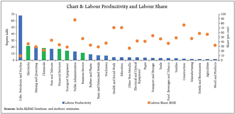

III.3 Investing in Digitalisation

Digitalisation can increase economic efficiency and competitiveness, creating new businesses and products, increasing financial inclusion, improving governance and reducing disparities. Deep penetration of telecom and internet, the Pradhan Mantri Jan-Dhan Yojana to connect people with bank accounts, creation of a unique identity number - Aadhar - for each resident and exponential growth in digital financial transactions combined with the focus on developing digital public infrastructure have laid the foundations of India’s digital economy – the India stack. Digitalisation increases productivity of both labour and capital, and thereby engenders a faster growth in total factor productivity.

We employ a dynamic factor model (DFM) to construct a time-varying index of digitalisation by extracting a common factor from data on all digital payments, number of internet users, number of mobile phone subscriptions, number of QR codes generated per 100 persons, credit to the software industry, investment in ICT (information and communication technology) and people employed in the ICT sector (Chart 9).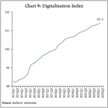

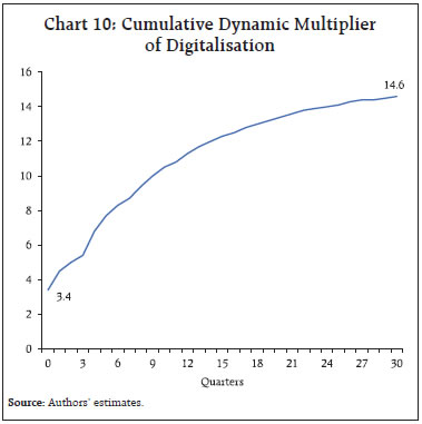We find that a one per cent rise in real DE increases digitalisation by 0.02 percentage points. A growth of 10.4 per cent in DE (as budgeted for 2024-25) can cause digitalisation to grow by 0.2 per cent. The impact and dynamic multipliers of digitalisation on the economy is estimated by using an auto-regressive distributed lag (ARDL) model. The impact multiplier on GDP is found to be 3.4 in response to a one per cent increase in digitalisation (Chart 10)⁵. The cumulative dynamic multiplier is estimated from the model at 15 in the long run. A growth of 0.2 per cent in the digitalisation index can raise GDP growth by about 130 bps in a year and by 2.8 percentage points over seven years.

III.4 Energy Efficiency

India has committed to achieve net zero emission target by 2070 for which the dependence on consumption of fossil fuel needs to be cut down. India has been able to reduce the energy intensity of GDP steadily due to both structural changes in the economy and technological efficiency. Based on the emission factors of different sources of energy, it has been estimated that a one per cent increase in the share of renewable energy in the energy mix reduces CO₂ emissions by around 0.63 per cent (RBI, 2023). India has made significant strides in renewable installed capacity and its share in total installed capacity is at 42 per cent (including large hydro). Based on several initiatives that have been taken towards climate risk mitigation and technological upgradation during recent years⁶, if the annual allocation towards climate mitigation is increased in a manner that 33 per cent of the annual allocation is invested in green energy augmenting technology every year, it will add to GDP growth by 10 basis points every year and 0.5 percentage points over the forecast horizon. As the horizon is lengthened, more gains accrue in terms of GDP growth. In the short-run, there may be a trade-off between climate mitigation and economic growth. In the medium term, however, there is no trade-off – mitigating climate risks is unequivocally beneficial for economic progress (Chart 11).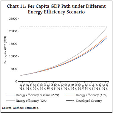

IV. The Model and Results

We consider a closed economy dynamic stochastic general equilibrium (DSGE) model comprising households, firms, the banking system, the fiscal authority and the central bank (Chart 12).

Households are of two types: one category has multiple sources of income from labour, interest earned from bank deposits, government bonds and dividends from the ownership of firms; the other category survives on labour income and direct transfers. On the production side, firms use labour, capital and energy as inputs in a competitive market environment. Banks intermediate all financial transactions among economic agents. Using the policy rate as its key instrument, the central bank follows an interest rate rule featuring interest rate smoothing and stabilisation of CPI inflation around its target and GDP growth around its trend. The fiscal authority uses alternative policy instruments such as spending on public consumption, transfers, investment on public capital goods, tax on labour income and private consumption. The issuance of government bonds constitutes public debt which is held by households and commercial banks. The government services its debt along with periodic interest payments. All the agents are rational and interact with each other in a dynamic environment. We solve the model to investigate the likely path of the debt to GDP ratio over the period 2024-25 to 2030-31 and explore alternative paths under four scenarios (Chart 13). Scenario 1 envisages the effect of an increase (5 per cent) in the employment level in relatively productive sectors as delineated in Section III.2. Scenario 2 considers the impact of a rise in energy efficiency. Scenario 3 explores fiscal policy intervention through capex towards greater digitalisation of the economy. Scenario 4 combines all the above outcomes simultaneously.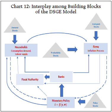

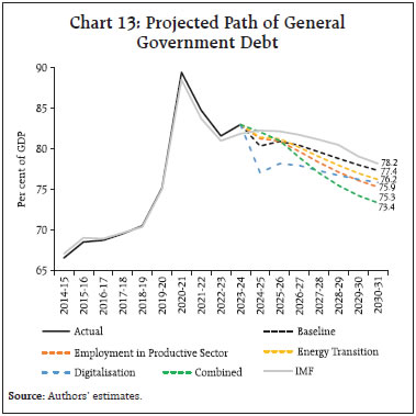Our baseline projection⁷ suggests that the debt-GDP ratio will chart a secular decline, reaching 77.4 per cent in 2030-31. In scenario 1, the debt-GDP ratio rises in the short-run, capturing the short-run trade-off, but falls thereafter to 75.3 per cent by 2030-31. Scenario 2 is similar to Scenario 1 in that the choice of energy-efficient transition is subject to short-run pain but it yields long-run gains by reducing the debt-GDP ratio to 76.2 per cent by 2030-31. In Scenario 3, digitalisation impacts the fiscal consolidation path through higher levels of productivity, taking the debt-GDP ratio at 75.9 per cent at the end of the forecast period. Scenario 4 combines all the measures and shows that the debt-GDP ratio declines to 73.4 per cent by 2030-31.

V. Conclusion

Policy wielders always face the trilemma of balancing climate goals, debt sustainability and operational feasibility within the political mandate (IMF Fiscal Monitor, 2023). The trade-offs are starker for developing countries for which developmental priorities dominate. We argue on the basis of our empirical findings in a general equilibrium framework that medium-term complementarities between judicious fiscal consolidation and growth outweigh the short-run costs. Spending on social and physical infrastructure, climate mitigation, digitalisation and skilling the labour force can yield long-lasting growth dividends.

Our simulations reveal that the general government debt-GDP ratio swerves below the projected path set out by the IMF in its latest Article IV consultation report for India⁸. With recalibration of government expenditure, the general government debt-GDP ratio is projected to decline to 73.4 per cent by 2030-31, around 5 percentage points lower than the IMF’s projected trajectory of 78.2 per cent. This is noteworthy as the debt-GDP ratio is projected to rise from 112.1 per cent in 2023 to 116.3 per cent in 2028 for advanced economies and from 68.3 per cent to 78.1 per cent for emerging and middle-income countries. It is in this context that we reject the IMF’s contention that if historical shocks materialise, India’s general government debt would exceed 100 per cent of GDP in the medium-term and hence further fiscal tightening is needed.

References

Alesina, A. & Ardagna, S. (2010). Large Changes in Fiscal Policy: Taxes versus Spending. Tax Policy and the Economy, Vol. 24. The University of Chicago Press, pp. 35–68.

Alesina, A., Carlo F., and Giavazzi, F. (2015). The Output Effect of Fiscal Consolidation Plans. Journal of International Economics, Vol. 96 (S1), pp. S19–S42.

Anand, R., Delloro, V., & Peiris, S. J. (2014). A credit and banking model for emerging markets and an application to the Philippines. In Proceedings of the 2014 BSP International Research Conference (No. 2).

Balasundharam, V; Basdevant, O; Benicio, D; Ceber, A; Kim, Y; Mazzone, L; Selim, H; Yang, Y. (2023). Fiscal Consolidation: Taking Stock of Success Factors, Impact, and Design, IMF Working Paper. No.63. March.

Banerjee, S. (2013) Essays on Inflation Volatility. Doctoral thesis, Durham University. Available in Essays on Inflation Volatility - Durham e-Theses

Banerjee, S., & Behera, H. (2023). Financial frictions, bank intermediation and monetary policy transmission in India. Economics of Transition and Institutional Change.

Banerjee, S., Basu, P., & Ghate, C. (2020). A monetary business cycle model for India. Economic Inquiry, 58(3), 1362-1386.

Baxter, M., & King, R. G. (1993). Fiscal policy in general equilibrium. The American Economic Review, 315-334.

Carrière-Swallow, Y., David, A. C., & Leigh, D. (2021). Macroeconomic effects of fiscal consolidation in emerging economies: New Narrative evidence from Latin America and the Caribbean. Journal of Money, Credit and Banking, 53(6), 1313-1335.

Colombo, E., Furceri, D., Pizzuto, P., & Tirelli, P. (2022). Fiscal multipliers and informality (No. 2022-2082). International Monetary Fund.

European Central Bank (2010). Economic and Monetary Developments. ECB Monthly Bulletin. June.

Gerali, A., Neri, S., Sessa, L., & Signoretti, F. M. (2010). Credit and Banking in a DSGE Model of the Euro Area. Journal of money, Credit and Banking, 42, 107-141.

Giavazzi, F. & Pagano, M. (1990). Can Severe Fiscal Contractions be Expansionary? Tales of Two Small European Countries. NBER Macroeconomics Annual. Vol. 5. MIT Press, pp. 75 – 122.

Guajardo, Jamie, Daniel Leigh, and Andrea Pescatori (2014). Expansionary Austerity? International Evidence. Journal of the European Economic Association, Vol. 12, No.4, pp. 949-968

Gupta, S., Clements, B., Baldacci, E., & Mulas-Granados, C. (2005). Fiscal policy, expenditure composition, and growth in low-income countries. Journal of International Money and Finance, 24(3), 441-463.

Hernández de Cos, Pablo, and Enrique Moral-Benito (2013). Endogenous Fiscal Consolidations. Fiscal Studies, Vol. 34, No. 4, pp. 491–515.

Hnatkovska, V and Lahiri, A. (2020) Money and Banking in Emerging Economies. Available in DSGE_OneSector_May2020.pdf. ubc.ca.

Ilzetzki, Ethan, Enrique G. Mendoza, and Carlos A. Végh (2013). How Big (Small?) are Fiscal Multipliers?. Journal of Monetary Economics, Vol. 60, No. 2, pp. 239-254.

International Monetary Fund (2014). Fiscal Multipliers: Size, Determinants, and Use in Macroeconomic Projections. Technical Notes and Manuals 14/04 (Washington: International Monetary Fund).

International Monetary Fund (2020). Mitigating Climate Change – Growth and Distribution-Friendly Strategies. World Economic Outlook October 2020 (Washington: International Monetary Fund).

Kim, J.I., Jean-Marc, A.B., Lee, K.Y., Toprak, H. H & Li, J (2021). Cross-Country Analysis of Program Design and Growth Outcomes: 2008–19. IEO Background Paper No. BP/21-01/01.

Kleis, M. & Moessinger, M.D. (2016). The Long-run Effect of Fiscal Consolidation on Economic Growth: Evidence from Quantitative Case Studies, ZEW - Leibniz Centre for European Economic Research, ZEW Discussion Papers. No.16-047.

Miyamoto, H., Gueorguiev, N., Honda, J., Baum, A., Walker, S., Schwartz, G., ... & Verdier, G. (2020). Growth impact of public investment and the role of infrastructure governance. International Monetary Fund, Washington, DC.

Reserve Bank of India (2023). Report on Currency and Finance: Towards a Greener and Cleaner India, May.

Saxegaard, M. M., Anand, R., & Peiris, M. S. J. (2010). An estimated model with macrofinancial linkages for India. International Monetary Fund.

Annexure

Model Appendix: Analytical Framework of DSGE Model

In Section IV, we present a stylised model of a closed economy that serves as an instrument to analyse the dynamics of debt. The model includes various building blocks, namely the household sector (HH), employment agency (EA), intermediate goods (IG) producing firms, final goods (FG) producing firms, capital goods (CG) producing firms, banking sector, the government and the central bank. The decision-making process of the agents and policy authorities is presented below. A.1 Household Sector A.1.1 Ricardian Households A.1.2 Non-Ricardian Households A.2. Producers A.2.1 Employment Agency Given the presence of two types of household agents, we consider a labour packer, alternatively employment agency, who aggregates two different types of labour using a CES-type aggregator, and converts into a uniform effective labour input as in Banerjee (2013). Additionally, we assume that the labour supplied by the Ricardian households is more efficient (skilled) than that of the non-Ricardian households (unskilled) as in Hnatkovska and Lahiri (2020). This skill gap is modelled by an efficiency wedge between Ricardian to Non-Ricardian labour andcaptured by the parameter μr(> 1). The technology for effective labour production is specified as: A.2.2 Capital Goods Producing Firms A.2.3 Intermediate Goods Producing Sector A.2.4 Final Goods Producing Firms A.3. Banking Sector A.3.1 Retail Branch The retail branch operates in a monopolistically competitive environment and set (a) the deposit rate for differentiated deposit contracts for the households, and (b) the lending rate for the IG firms, subject to interest rate adjustment costs. While solving their optimal interest rate setting problem, they face upward sloping deposit supply function and downward sloping loan demand function. A.3.2 Wholesale Branch A.4. Central Bank A.5. Fiscal Authority In case of fiscal authority, the nominal budget constraint of the government is: A.6. Closing the Model Under the assumption of symmetric equilibrium and using market clearing conditions of the factor markets, goods market and credit market, the model is closed with the following resource constraint that specifies the aggregate demand of the underlying economy: A.7. Exogenous Shocks A.8. Solving the Model All the decision rules derived from the first principle of the dynamic optimisation and the resource constraints are taken together and log-linearised around the steady state of the respective variables. Using a plausible set of parameterisation, the linearised system of equations is solved. The calibrated parameters are in line with Indian macroeconomic data, economic characteristics and policy mandates.

^{^} The authors are from the Reserve Bank of India. The views expressed in this article are those of the authors and do not represent the views of the Reserve Bank of India.

¹ Dahiya, R. (2024). An NLP Analysis of the Budget (Forthcoming).

² Empirical evidence on these predictions is mixed as multipliers in developing countries could also be reduced by larger precautionary savings stemming from an uncertain macroeconomic environment, low efficiency of public expenditure, lower fiscal policy credibility and a large informal economy (Miyamoto et al., 2020; Ilzetzki, Mendoza and Vegh, 2013; Colombo et al., 2022).

³ The general government debt ratio stands at 81.6 per cent of GDP in 2023-24 (BE).

⁴ The India KLEMS database, constructed by the Reserve Bank of India, consists of inputs (employment, labour quality, capital stock, capital composition, consumption of energy, material and services), output (gross value added; gross output) and total factor productivity (TFP) estimates from 1980-81 to 2021-22 for 27 industries.

⁵ It may be noted that it took five years period for digitalisation to increase by one per cent.

⁶ Using an environmental Solow-type growth model, it has been shown that India’s objective of becoming an advanced economy by 2047 is possible by enhancing the labour augmenting and energy augmenting technology growth by 10 per cent and 6 per cent, respectively (RBI, 2023).

⁷ In the baseline, real GDP growth is projected at 7.3 per cent per annum during the forecast period. CPI inflation is projected at 4.3 per cent per annum and remains stable at that level for the alternative scenarios.

⁸ Staff Report for the 2023 Article IV Consultation for India; IMF Country Report Number 23/426; December 2023.

⁹ Given the presence of public sector units (PSUs) and public sector banks (PSBs) in the economy, we assume that the government owns the firms and banks partially. Hence, a portion of profit of the firms and banks is reaped by the government in the form of non-tax revenue. The rest of it accrues to the Ricardian households.

¹⁰ For an empirically plausible analysis, we disaggregate the productivity shock into two components, namely shocks to total factor productivity and labour augmenting technology, and dissect their differential impacts on the business cycles.