by Shesadri Banerjee, Harendra Behera and Michael Debabrata Patra^{^}

Dynamic Stochastic General Equilibrium (DSGE) models have become the workhorse organising frameworks among modern central banks for formulating and communicating monetary policy. A prototype DSGE model for India with open economy and New Keynesian properties estimated over the period 2004-05:Q1 to 2022- 23:Q4 reveals that aggregate demand has become more elastic to changes in the real rate of interest after the shocks of the pandemic and the war in Ukraine; and disinflation has become costlier in terms of output sacrificed.

Introduction

Dynamic Stochastic General Equilibrium (DSGE) models have become the workhorse organising frameworks among modern central banks for formulating and communicating monetary policy. Built on microeconomic foundations to characterise intra- and inter-temporal choices, these models assign a key role to the expectations of economic agents about the uncertain future, making them dynamic. DSGE models typically involve a detailed specification of shocks – surprises in the form of mismatches between expectations and outcomes – that give rise to economic fluctuations, and this renders these models stochastic. They are also able to capture interactions between the behaviour of economic agents and policy actions within their general equilibrium structure. In response to criticism that DSGE models failed to predict the global financial crisis (Solow, 2010; Stiglitz, 2018; Blanchard, 2018), these models have evolved to incorporate financial intermediation and frictions, labour market mismatches, household heterogeneity and macroprudential policy tools in order to reflect emerging realities (Roger and Vleck, 2011; Galvao et al., 2016; Ravn and Sterk, 2016; Ghironi, 2017; Christiano et al., 2018; Kaplan et al., 2018). In essence, DSGE models serve the purposes of story telling, policy evaluation and forecasting in a framework that connects business cycle fluctuations and stabilisation policies (Del Negro and Schorfheide, 2013).

Drawing on influential work on the theme¹, we sketch out a prototype DSGE model for India with open economy and New Keynesian properties². We estimate the model over the period 2004-05:Q1 to 2022-23:Q4³ to assess the structural changes in the economy and shifts in key wielding parameters characterising the conduct of monetary policy before the twin shocks of the pandemic and the war in Ukraine, and after them. The economy is conceptualised as comprising a representative household, which maximises the present value of satisfaction as a consumer, subject to a budget constraint; a representative firm maximising a discounted stream of profit as a producer in response to prospects of demand for its production; and the central bank which follows a feedback rule in the use of its policy instruments to achieve its mandate. All the agents are rational⁴ and engage in collective interplay, which shapes demand-supply adjustments over time. This adjustment is, however, exposed to the uncertainties of random shocks emanating from changes in productivity, aggregate demand, import prices and the external sector.

We attempt a baseline estimation for the sample period 2004:Q1 – 2019:Q4 (pre-pandemic), and then extend the sample to include the pandemic period (post-pandemic). Our results suggest that (i) aggregate demand has become more elastic to changes in the real rate of interest; and (ii) more output has to be given up for reducing inflation in the post-pandemic period relative to the pre-pandemic period. In Section 2, we provide some stylised facts as a backdrop for a broad description of the model in Section 3. The choice of data and period of study, and model estimation are discussed in Section 4. Section 5 presents the results and highlights the main shifts in the features of the Indian economy between pre- and post-pandemic periods. Section 6 concludes with some policy perspectives.

II. Stylised Facts

Commencing in 2003, the Indian economy experienced a phase of high growth relative to trend that lasted up to 2007 before it was interrupted by the global financial crisis (GFC). Real GDP growth averaged 7.9 per cent during this period. The economy slowed down in the immediate aftermath of the GFC to 3.1 per cent in 2008-09, but recovered during 2009-2013 and real GDP growth averaged 6.0 per cent. This recovery co-existed with double digit inflation (13.3 per cent during July 2009 - July 2010 and 10.1 per cent during June 2012 – November 2013), which moderated only with the institution of the pre-conditions for a flexible inflation targeting (FIT) framework. Average inflation was 3.9 per cent during 2016-20 with the de jure establishment of the FIT regime, in alignment with the inflation target of 4 per cent within a tolerance band of +/- 2 per cent around it.

With the onset of the COVID-19 pandemic which was a ‘once in a century’ shock, India suffered among the deepest contractions in the world in 2020-21, with GDP declining by 23.4 per cent in Q1 (Chart 1). Fiscal stimulus and various conventional and unconventional monetary and liquidity measures were undertaken to protect “life and livelihood of people”⁵. In response, the economy started recovering in the second half of 2020-21, although GDP trailed below pre-pandemic levels. In early 2022, as inflationary pressures eased and signs of a recovery gained traction, the outbreak of war in Ukraine upended the situation and altered the trajectory of the world economy drastically. International commodity prices, especially the price of crude oil, shot up by more than 80 per cent during 2021-22. Supply chain pressures built up both globally and domestically, leading to mounting input cost pressures. Under the impact of these developments, CPI headline inflation breached the upper tolerance level of 6 per cent and stayed above it for ten months consecutively, dipping below to 5.7 per cent in March 2023 and to 4.7 per cent in April. For the year 2022-23 as a whole, inflation averaged 6.7 per cent, up from 5.5 per cent a year ago. It is expected to ease to 5.1 per cent in 2023-24⁶. Real GDP growth at 7.2 per cent in 2022-23 on top of 9.1 per cent in 2021-22 and is projected to ease to 6.5 per cent in 2023-24.

In this highly uncertain and rapidly changing macroeconomic environment, therefore, the question that is drawing animated discussion is: have the key structural relationships and/or driving forces in the Indian economy changed? We investigate this question through the lens of a prototype DSGE model that is presented and estimated in the following sections.

III. Model Environment

In our DSGE world, the household’s consumption basket is a composite of domestically produced and imported goods and services. Consumption essentially involves a trade-off between current and future spending, subject to the degree of habit formation and the sensitivity of consumption demand to the expected real rate of interest. The household provides labour to the firm, which is the only input for production.

Turning to the production side, both domestic producers and importers exercise pricing power but face nominal rigidities like staggered price setting (Calvo, 1983)⁷. As regards the firm’s profit maximising behaviour, we depict it through two supply relationships taking the form of New Keynesian Phillips Curves (NKPC) – one for domestically produced goods and services and the other for imported ones. These equations connect inflation dynamics of each category to cost pressures (real marginal cost for domestic production and markups on imported goods that drive a wedge between landed costs and retail prices), inflation inertia, i.e., the magnitude of past inflation feeding into current inflation, staggered price setting or price stickiness and a discount factor which measures the influence of inflation expectations in determining current period inflation. Consumer price inflation is aggregated as the weighted average of domestic and imported inflation, with the weights representing the degree of trade openness and home bias⁸.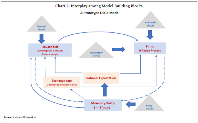

Monetary policy is conducted according to an interest rate rule that reacts more than proportionately to changes in inflation relative to target. The rule also stabilises output around its potential level (Taylor, 1993). There is a considerable degree of interest rate smoothing in which the policy rate is adjusted in a sequence of small steps and gradually.

To reiterate, in addition to staggered price setting, the model also features several structural rigidities as suggested in the business cycle literature such as (i) habit formation in consumption; (ii) indexation of prices set by firms to past inflation; (iii) uncovered interest rate parity (UIP) with external risk premium⁹; and (v) short-run deviations from the law of one price (LOOP)¹⁰ (Adolfson et al., 2007; Anand et al., 2010).

The model incorporates a number of shocks like changes in the firms’ productivity, importers’ markups, risk in international financial markets, monetary policy, and disturbances from the foreign economy such as changes in global GDP, global CPI inflation and the US Federal Funds rate (Chart 2). All of these variables are assumed to be determined outside the model and to follow a first-order autoregressive process, i.e., their current values depend on their oneperiod lagged realisations¹¹.

IV. Model Estimation

We calibrate some of the model parameters from the existing body of work on the Indian economy and estimate the others as they can vary spatially and over time. We consider eight macro-economic indicators, i.e., output gap measured as the deviation of actual GDP from its trend (per cent); CPI inflation measured as year-on-year (y-o-y) changes; the weighted average call money rate as a proxy for the policy rate; changes in the nominal exchange rate of the Indian rupee vis-à-vis the US dollar (seasonally adjusted annualised rate or saar); global GDP growth (y-o-y); world CPI inflation rate (saar); changes (y-o-y) in the terms of trade measured by the ratio of prices of import to export unit values; and the US Fed funds rate.

In our estimation routine, we apply Bayesian methods to estimate the following parameters: (i) degree of trade openness and substitutability between domestic and imported goods; (ii) (inverse) elasticity of substitution between current and future consumption and the degree of habit formation; (iii) price stickiness and past inflation indexation; (iv) coefficients of the Taylor-type policy rule; (v) first order persistence coefficients which indicate how long a shock to the system lasts; and (vi) the standard error of the shocks, which measures the degree of uncertainty the economy is facing.

We employ a two-step estimation procedure. In the first step, probable values of estimable parameters of the model are set up on the basis of a priori knowledge and proximate guidance in the literature as initial starting points or ‘priors’ with theoretically plausible probability density functions, since they are unknown or unobserved in real life¹². For instance, the beta distribution is used for the degree of price stickiness, while the inverse gamma distribution is specified for the standard errors of the shocks because they take only positive values. We obtain the posteriors in five steps. First, the economic relationships and the eight observable variables with measurement equations are written in a Kalman filter recursion form. Second, the log likelihood function of the relevant parameter vector is constructed. Third, the log posterior kernel is derived from the probability distributions assigned to the priors. Fourth, the mode of this posterior kernel is computed by using standard numerical optimisation routines. Finally, a Gaussian approximation is constructed in the neighbourhood of this posterior mode by employing the Markov Chain Monte Carlo-Metropolis-Hastings (MCMC-MH) algorithm. We take 100,000 replications to implement the MH algorithm in which the first 50 per cent of the ‘burn-in’ observations are discarded to reduce the importance of starting values. Four parallel chains are used in the MCMC-MH algorithm with an acceptance rate of 26 per cent. This algorithm simulates the smoothed histogram that approximates the posterior distributions of parameters of our interest. The univariate and multivariate diagnostic statistics show convergence when comparing between and within moments of multiple chains (Brooks and Gelman, 1998). Based on the simulation exercise, the key impulse responses of the exogenous shocks to productivity and monetary policy are presented (Chart 3).

It is observed that a positive shock to productivity increases output and reduces real marginal cost that, in turn, lowers domestic inflation. Following the decline in inflation, the policy rate is reduced. In case of a positive shock to the policy rate, the rise in the policy rate increases the cost of current consumption vis-à-vis future consumption. Hence, consumers cut down present consumption demand which, in turn, entails a reduction in firms’ production and thus, output shrinks. The real marginal cost of production drops and this leads to a decline in inflation. A 100 basis points (bps) rise in the policy rate is estimated to reduce the output gap by 50 bps and inflation by 45 bps over eight quarters.

V. What has Changed in India after the Pandemic?

Given the sheer scale of the impact of the pandemic and the war, it is worthwhile to look for structural changes in the economy. The standard errors of shocks have increased considerably, indicative of the unprecedented nature of the shocks (Chart 4). Uncertainty related to productivity and demand has gone up by 2.9 and 1.5 times, respectively, in India and by 2.3 times for global output, in comparison with pre-pandemic levels.

On the demand side, there is a shift in the preference pattern of consumers. First, the substitutability between the current and future consumption has increased, revealing that the households have become more risk averse and prone to build up precautionary savings; and second, the habit of past consumption has lesser effect on current consumption. Although the share of imports in the consumption basket remains the same, its substitutability with domestic components has increased. These parametric shifts in household behaviour underline the change in the sensitivity of aggregate demand to interest rate changes, which during the period of twin shocks helped the transmission of policy impulses to support demand. Our estimation results show that interest rate sensitivity of aggregate demand has increased from 0.44 to 0.48.

On the supply side, changes are observed in the price setting behaviour of domestic firms in contrast to importing firms. First, the indexation of past inflation by domestic retailers has declined relative to importers. This implies that domestic firms have become more forward looking. Second, the price of domestic goods has become stickier, while price stickiness has dropped for imported goods. This reveals a structural shift in the pattern of price setting, pointing to a decline in the sensitivity of inflation to demand. The responsiveness of inflation to real marginal cost, formally the slope of the NKPC has declined from 0.29 (pre-pandemic) to 0.24 (post-pandemic). This flattening of the Phillips curve makes the inflation-output trade-off costlier – every unit of disinflation costs more in terms of the sacrifice of output after the pandemic than before it¹³.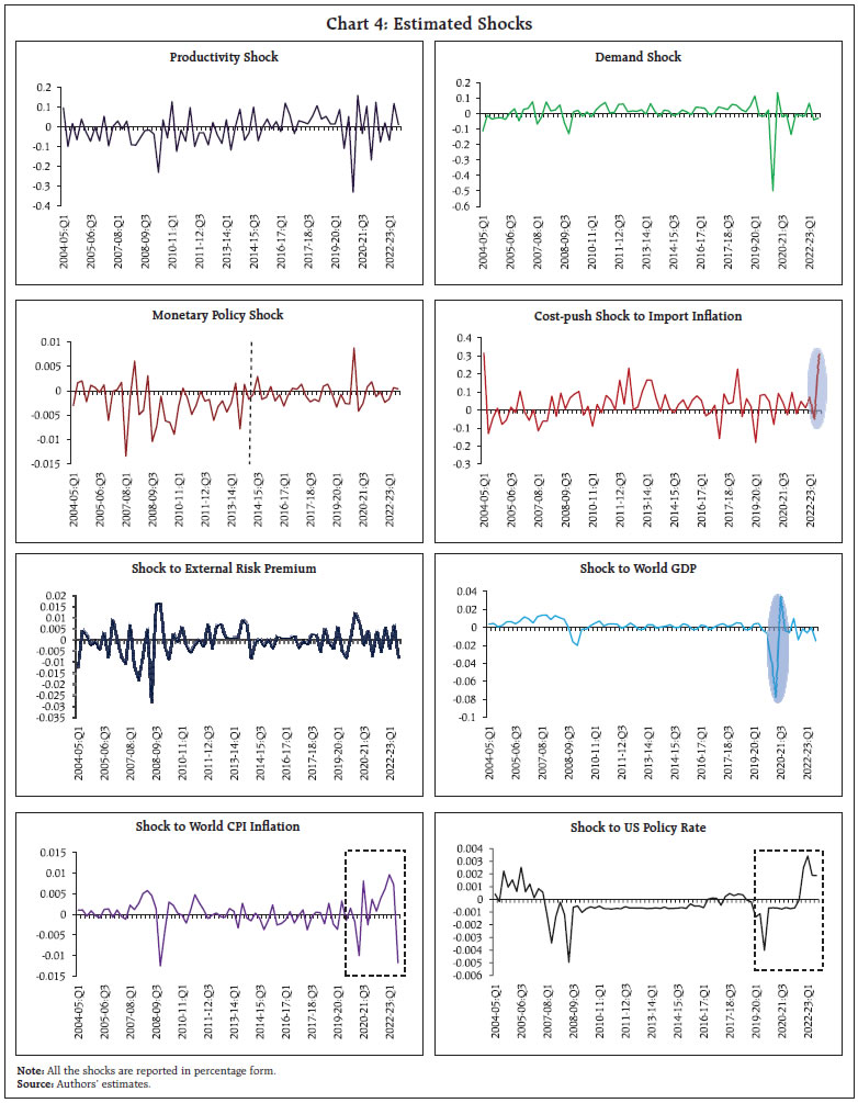

On the policy front, the monetary policy rule appears to be stable with a modest increase in interest rate smoothing and output gap coefficients¹⁴, and a mild decline in the inflation stabilising coefficient. Such changes in the coefficients can be attributed to the accommodative stance of monetary policy during the pandemic period and the current stance of withdrawal of accommodation that has been preferred over aggressive rate hikes.

VI. Conclusion

The world is not the same after the overlapping shocks of the pandemic and the war in Ukraine. What has changed and how these shifts can be measured is our motivation in an environment in which evidence is still forming and the standard relationships that capture the interaction of monetary policy with the rest of the economy are fluid. Two salient results would inform the setting of monetary policy going forward. First, higher sensitivity of aggregate demand to changes in the real rate of interest that we find in the post-pandemic period indicates that smaller magnitudes of policy rate increases may be needed to quell inflationary pressures than in the pre-pandemic period. Second, the flattening of the Phillips curve points to higher costs of stabilisation than in the past. This will make disinflation strategies more costly in the future. As regards the finding that the transmission of cost pressures to inflation is more muted now than before, a caveat is in order: depressed demand conditions prevailed during the pandemic, and hence, our results may be subject to an end-point bias. Nonetheless, if the pandemic experience gets fully incorporated into expectations, the sacrifice ratio is set to increase – it will be costlier in the future for monetary policy to ensure price stability than in the pre-pandemic period. The conduct of monetary policy after the pandemic has become more complicated than before.

References

Adolfson M, S Laséen, J Lindé and M Villani (2007), ‘Bayesian Estimation of an Open Economy DSGE Model with Incomplete Pass-Through’, Journal of International Economics, 72(2), pp 481–511.

Blanchard, O. (2018). On the Future of Macroeconomic Models. Oxford Review of Economic Policy, 34(1-2), 43-54.

Brooks, S. P., & Gelman, A. (1998). General methods for monitoring convergence of iterative simulations.

Journal of Computational and Graphical Statistics, 7(4), 434-455.

Calvo, G. A. (1983). Staggered prices in a utility-maximizing framework. Journal of Monetary Economics, 12(3), 383-398.

Ca’ Zorzi, M. and Rubaszek, M. (2017) Exchange rate forecasting with DSGE models, Journal of International Economics, vol. 107, p. 127 – 146.

Christiano, L. J., Eichenbaum, M. S., and Trabandt, M. (2018). On DSGE Models. Journal of Economic Perspectives, 32(3), 113-140.

de Menezes Linardi, F. (2016). Assessing the fit of a small open-economy DSGE model for the Brazilian economy. Central Bank of Brazil Working Paper, 424.

Del Negro, M., & Schorfheide, F. (2013). DSGE model-based forecasting. In Handbook of economic forecasting (Vol. 2, pp. 57-140). Elsevier.

Galí, J. and Monacelli, T. (2005) Monetary Policy and Exchange Rate Volatility in a Small Open Economy, The Review of Economic Studies, Volume 72, Issue 3, July, Pages 707–734, https://doi.org/10.1111/j.1467-937X.2005.00349.x

Galí, J. (2015). Monetary policy, inflation, and the business cycle: an introduction to the new Keynesian framework and its applications. Princeton University Press.

Galvao, A. B., Giraitis, L., Kapetanios, G., & Petrova, K. (2016). A time varying DSGE model with financial frictions. Journal of Empirical Finance, 38, 690-716.

Ghironi, F. (2018). Macro needs micro. Oxford Review of Economic Policy, 34(1-2), 195-218.

Justiniano A and B Preston (2010), ‘Monetary Policy and Uncertainty in an Empirical Small Open Economy Model’, Journal of Applied Econometrics.

Kaplan, G., Moll, B., & Violante, G. L. (2018). Monetary policy according to HANK. American Economic Review, 108(3), 697-743.

Kollmann, R. (2002). Monetary policy rules in the open economy: effects on welfare and business cycles. Journal of Monetary Economics, 49(5), 989-1015.

Lawrence J. Christiano & Martin Eichenbaum & Charles L. Evans, 2005. “Nominal Rigidities and the Dynamic Effects of a Shock to Monetary Policy,” Journal of Political Economy, University of Chicago Press, vol. 113(1), pages 1-45, February.

Lucas Jr, R. E. (1972). Expectations and the Neutrality of Money. Journal of Economic Theory, 4(2), 103-124.

Lucas Jr, R. E. (1976, January). Econometric policy evaluation: A critique. In Carnegie-Rochester conference series on public policy (Vol. 1, pp. 19-46). North-Holland.

Muth, J. F. (1961). Rational expectations and the theory of price movements. Econometrica: Journal of the Econometric Society, 315-335.

Ravn, M., & Sterk, V. (2016). Macroeconomic fluctuations with HANK & SAM: An analytical approach. centre for Macroeconomics discussion papers 1633. University college London.

Reserve Bank of India. (2022). Monetary Policy Report, September.

Roger, S., & Vlček, J. (2011). Macroeconomic costs of higher bank capital and liquidity requirements. IMF Working Papers 2011/103, International Monetary Fund.

Saxegaard, M. M., Anand, R., & Peiris, M. S. J. (2010). An estimated model with macrofinancial linkages for India. International Monetary Fund.

Sbordone, A. M., Tambalotti, A., Rao, K., & Walsh, K. J. (2010). Policy analysis using DSGE models: an introduction. Economic policy review, 16(2).

Schmitt-Grohé, S., & Uribe, M. (2003). Closing small open economy models. Journal of international Economics, 61(1), 163-185.

Smets, F., & Wouters, R. (2003). An estimated dynamic stochastic general equilibrium model of the euro area. Journal of the European economic association, 1(5), 1123-1175.

Smets, F. and Wouters, R. (2007). Shocks and Frictions in US Business Cycles: A Bayesian DSGE Approach, American Economic Review, American Economic Association, vol. 97(3), pages 586-606, June.

Solow, R. (2010). Building A Science of Economics for the Real World. House Committee on Science and Technology Subcommittee on Investigations and Oversight, 20.

Stiglitz, J. E. (2018). Where Modern Macroeconomics Went Wrong. Oxford Review of Economic Policy, 34(1- 2), 70-106.

Appendix

In this section, we describe our modelling framework drawing from the literature (Linardi, 2016; Justiniano and Preston, 2010; Anand et al., 2010). The building blocks are as follows: households, domestic producers, retailers, external block, and the monetary authority.

A.1. Households

Households are assumed to maximise the present value of the expected utility as:

Given that the only available assets are one-period domestic and foreign bonds; household’s optimisation takes place subject to the flow budget constraint:

The household’s optimisation problem requires allocation of expenditures across all types of domestic and foreign goods, both intra-temporally and inter-temporally. This yields the following set of optimality conditions.

Allocation of expenditures on the aggregate consumption bundle, optimal labour supply, and portfolio choice are determined by:

A.2. Domestic Producers

There is a continuum of monopolistically competitive domestic firms producing differentiated goods. Calvo-style price setting is assumed along with the indexation to past domestic goods price inflation. Hence, in any period t, a fraction (1 - θ_H) of firms set prices optimally, while the rest of firms (0 < θ_H < 1) adjust their prices according to the indexation rule:

A.3. Retail Firms

Retail firms import foreign-produced differentiated goods for which the law of one price holds at the docks. In determining the domestic currency price of the imported good, firms are assumed to be monopolistically competitive. They face a Calvo-style price-setting problem allowing for indexation to past inflation. Hence, in any period t, a fraction (1 - θ_F) of firms set prices optimally, while the other fraction 0 < θ_F < 1) of firms adjust their goods prices according to an indexation rule analogous to (8). The Dixit-Stiglitz price aggregator evolves as:

A.4. External Block

The uncovered interest rate parity condition follows from the asset-pricing conditions (6) and (7) that determine domestic and foreign bond holdings, and connect the relative movements of the domestic and foreign interest rate to changes in the nominal exchange rate:

6.5 Monetary Policy

The central bank follows a feedback rule according to which the interest rate responds to deviations of inflation and output gap from their respective steady-state levels.

We close the model with goods market clearing condition using symmetric equilibrium; and equilibrium condition for the balance of payments. We assume that the fiscal authority is: (i) pursuing a zero debt policy with net supply of Dt=0 ; and (ii) imposing taxes equal to the subsidy as required to eliminate the steady-state distortion emerging from imperfect competition in the domestic and imported goods markets. Finally, the time paths of foreign variables are considered as autoregressive processes of order one.

^{^} The authors are from the Reserve Bank of India. The views expressed in this article are those of the authors and do not represent the views of the Reserve Bank of India.

¹ Smets and Wouters, 2003; 2007; Christiano et al., 2005; Monacelli, 2003; Gali and Monacelli, 2005; Justiniano and Preston, 2010; Anand et al., 2010; and Ca’ Zorzi et al., 2017.

² As discussed in Gali (2015), New Keynesian elements are incorporated via the assumptions of imperfectly competitive commodity markets and staggered price-setting behaviour of firms; the economy also engage in foreign trade and its economic agents can hold foreign bonds, giving it an open economy character.

³ The choice of 2004-05 as the initial starting point coincides with it being the base year for both national accounts and wholesale price index. The terminal point is determined by data availability.

⁴ Rationality implies that individuals make decisions based on all available information and learn from past events (Muth, 1961; Lucas, 1972, 1976).

⁵ Das, S., (2020). Indian Economy at a Crossroad: A view from Financial Stability Angle. Speech delivered at the 7th SBI Banking & Economics Conclave, State Bank of India, July 11, URL: https://rbidocs.rbi.org.in/rdocs/Speeches/PDFs/SBIS4443A645BE9C44F3B45F1B3AA2018EDF.PDF

⁶ Resolution of the Monetary Policy Committee (MPC) June 6-8, 2023, Reserve Bank of India (RBI).

⁷ When a firm sets a price for its product, there is a constant probability that it will be able to reset the price independent of the time since it was last reset.

⁸ Note that in the case of zero indexation to past inflation, absence of habit formation and zero degree of trade openness, the framework will reduce to the standard closed economy New Keynesian model with a dynamic IS curve, a forward looking NKPC and an interest rate rule.

⁹ Under the UIP condition, the difference in interest rates between two countries will equal to the expected change in their exchange rates.

¹⁰ In the model, the ‘law of one price gap’ is the difference between the foreign currency price and the domestic currency price of imports.

¹¹ Detailed modelling framework is provided in the Appendix.

¹² Probability density function is a statistical measure used to gauge the likely outcome of a discrete value of a variable.

¹³ The recursive estimates from the model show a significant fall in the response of inflation to marginal cost at the time of pandemic leading to a lower slope coefficient in the post-pandemic period. However, the slope has started rising incrementally in subsequent period.

¹⁴ Despite the accommodative stance of monetary policy in massive scale to tackle severe slacks in the economy, the coefficient of output gap in the policy reaction function has increased marginally on account of rise in amplitudes of output gap. Moreover, the post-pandemic sample contains mostly the periods of sustained reduction in the policy rate generating a higher value of interest rate smoothing parameter.

¹⁵ Households are assumed to have identical initial wealth, so that each faces the same periodical budget constraint, and therefore, make identical consumption and portfolio decisions.

¹⁶ This functional form ensures stationarity of the foreign debt level in a log-linear approximation to the model.