by Dipak R. Chaudhari, Akanksha Handa, Priyanka Upreti, and Saurabh Ghosh^ The realty sector plays a crucial role in India in terms of employment generation, savings in physical form, contribution to the country’s GVA, and even as an early warning indicator. However, low-frequency traditional data and the lag in data releases make its active use in policy-making difficult. We aim to bridge this challenge by constructing a realty sector activity indicator using a variety of high-frequency indicators and a dynamic factor model. Us ing this indicator, we quantify the impact of realty sector developments on economic activity, its first and second-rounds effects across business cycles. Introduction The realty sector plays a pivotal role in the Indian economy. This sector provides the second-largest employment, after the agriculture sector, for both skilled and unskilled labourers (84 per cent share of informal workers). Moreover, the realty sector produces employment opportunities to a large fraction of immigrant workers from several parts of the country (GOI, 2021). The realty sector is also linked to upstream and downstream industries, creating second-round positive spillover effects on them. In addition, the realty sector1 provides an essential avenue for savings in physical form. The average household in India holds 77 per cent of its total assets in real estate which comprises of constructions for residential purposes, farm and non-farm activities, recreational facilities, rural and urban land, etc. (Ramadorai, 2017). The high level of real estate holdings by Indian households could indicate their need for real estate investments in addition to usual consumption needs. The available literature from similar emerging market economies (EMEs) suggests that construction activities have a positive relationship with economic growth, however, it may be a contemporaneous, lead or lagged association. For instance, Berk and Bicen (2017) examined the relationship between investment in the construction sector and gross domestic product (GDP) growth and found that the former leads to economic growth. Ahmad et al. (2019) examined the interactions between the construction sector and urbanisation, energy consumption, economic growth, and carbon emissions for the Chinese economy and found that the construction sector leads to urbanisation, which is a key driver of economic growth. Hung et al. (2019) analysed the linkages of the construction sector with the total output of the economy using a multi-regional input-output table for Hong Kong and found similar results. In the Indian context, there exists limited literature that has examined the relationship of construction activities with economic growth. Tiwari (2011) studied the relationship between construction activity and economic growth and found the existence of bidirectional causality between economic growth and construction activities. Kumar and Choudhary (2014) empirically investigated the effect of housing investment on GDP and found a strong positive correlation among housing, GDP and employment. Using a production function based approach, Mallick and Mahalik (2010) found a positive impact of construction on economic growth. Since a significant portion of the realty sector and its feedback effects relate to the informal sectors in India, data availability issues pose a considerable challenge to pre-emptive policy research in this domain. We aim to address this gap by using both conventional and unconventional data sources. In this vein, we start with a preliminary assessment of available high-frequency indicators that could be related to the real estate sector in India. Second, we attempt to find a latent common factor underlying these series that represent realty sector developments and construct a dynamic factor for housing (DFH), which can be used for policy research. Finally, we run empirical tests using DFH, construction gross value added (GVA), and GVA net of construction to evaluate the efficacy of DFH in policy-research. The rest of the study is organised as follows: Section II takes a deep dive into the realty sector with the help of conventional and unconventional high-frequency data. Section III explains data dimension reduction, nowcasting and other empirical findings. Section IV concludes the study and discusses policy implications. II. Data and Trends India is a services-driven economy, with the services sector accounting for more than 60 per cent of total GVA. The construction sector, which accounts for around 8 per cent of total GVA, recorded the steepest decline, by around 50.3 per cent as sales and new launches contracted during the first quarter of 2020-21, primarily due to lockdown and sluggishness of consumer sentiments during pandemic period (MOSPI, 2020). Consumer Pyramid database of Centre for Monitoring Indian Economy (CMIE) indicates that unemployment figures for the construction sector were amongst the highest in various industries during the lockdown. Another component of services i.e., financial, real estate and professional services, witnessed a decline in the first and the second quarter of 2020-21 as compared to the same periods in 2019-20. However, there are two problems with the conventional dataset: (a) it is of quarterly frequency, and (b) it is difficult to gauge the direct and indirect impact of an adverse-shock or slowdown in the realty sector on the overall economic data, especially for identifying the impact on the supply side vis-à-vis the demand side. We, therefore, considered a slew of available high-frequency indicators that are related to the realty sector in India. These include variables such as housing prices, credit and profits of real estate companies that are mostly sourced from CEIC. Available corporate performance data (from CMIE Prowess dataset) and stock market indices (Bloomberg Data) indicate mixed evidence. While the former shows signs of deterioration, the realty stock indices have surpassed their pre-COVID levels, indicating future promises for the sector. Further, we included high-frequency variables such as cement and steel production (CEIC database), which may be related to the construction sector through upstream or downstream supply chain linkages. Since steel and cement have a combined weight of only 23 per cent in IIP core2 and there are other industries i.e., electricity, coal and crude oil too that have a direct and indirect impact on the realty sector, IIP core is used as a separate variable. Moreover, since many of these are bulk inputs and are commonly transported by railways, we have also included different components of railway freight in our analysis. In doing so, we realized that total freight and freight (tonne) per KM have quite different cycles (Annexure Chart 1.B). Therefore, we preferred to retain both for our analysis. Finally, in view of the infotech revolution and stock market developments, we use a few unconventional variables in our analysis. These include Realty Index (adjusted for broad market movements) and Google Search Propensity related to the realty sector. Chart 1 shows the trends in the composite real estate search propensity indicator which is calculated by taking weighted average of search propensity of some keywords related to commercial property (real estate, commercial property, residential property, 99 acres, Magicbricks, No Broker), weights being the inverse of the variance of search propensity of each keyword. This search propensity indicates the ratio of the total number of searches containing a particular keyword relative to the total number of searches during that time period, which is then normalised between 0-100. 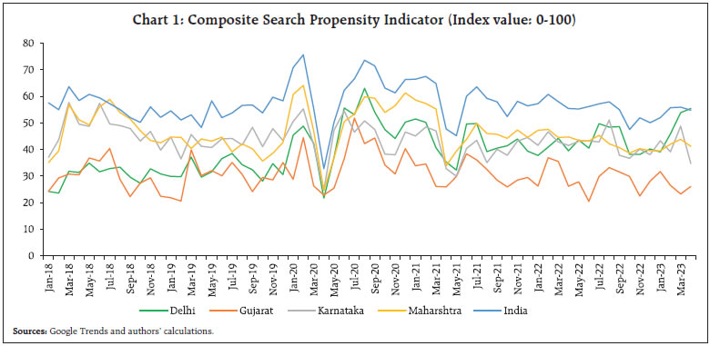 While these variables indicate divergent movements in the short run, our analyses indicate that there could be a hidden common factor that drives all realty sector-related variables in the long run. In the following empirical section, we intend to decipher this common factor based on a select list of variables. III. Empirical Findings We analyse the above set of variables that are related to the realty sector across different phases of business cycles. Here, we have focused on the post-global financial crisis (GFC) period, i.e., 2009 onwards. The period of the study is from March 2009 to December 2020. We evaluated the correlation of the above-mentioned variables with construction sector GVA and overall GDP and computed dynamic correlations. III.1. Dating of GDP Growth Cycle and Growth Rates of Select Housing Variables Following Bhadury et al. (2020), we identify the GDP growth cycle over the last two decades, by using the 1st and 4th quartiles of GDP growth, i.e., the lowest 25 per cent and the highest 25 per cent of growth rates. In addition, we apply a few censor rules to clearly recognise the turning points in the GDP cycle. We observe a common trend/co-movements in the construction-related variables, namely steel, cement and railway freight. The other variables, namely housing prices, stock indices (adjusted realty index) and housing credit appear to be mostly pro-cyclical (Annexure Chart 1.A). Google search propensity index has also shown divergence from the phases of the business cycle indicating more search intensity of the terms related to the real sector during slowdown phases. Next, we carry out the correlation analysis for our quarter-over-quarter (Q-o-Q) seasonally adjusted annualised growth of the construction-GVA as it is a more representative indicator for output in the real estate sector (Table 1). The exercise is conducted for the period Q2:2009 to Q4:2020, with 46 observations, at different leads and lags of construction GVA. The variables have a Contemporaneous (‘C’), Leading (‘L+’) or Lagging (‘L-’) relationship with the construction GVA. It can be clearly seen from Table 1 that steel, cement production, Index of Industrial Production (IIP) core, Sensex-adjusted Realty Index and rail freight exhibit high contemporaneous correlation with construction GVA. Housing prices are found to be significantly correlated with past construction GVA. From these two exercises, five variables are found to be having a high contemporaneous relationship with construction GVA and one variable is found to be having a lagging relationship with construction GVA3. The variables are steel, cement production, IIP core, rail-freight, rail-freight (ton) per KM, adjusted realty index, and housing prices, which were considered for extracting the common factor in a dynamic factor model (Annexure Chart 1.A and 1.B). | Table 1: Correlation of Selected Variables with Construction GVA | | Variables | Construction GVA(-t) (Lagging Relationship) | Construction GVA (contemporaneous relationship) | Construction GVA(+t) (leading relationship) | Comments | | Housing credit | 0.1336 | -0.1094 | -0.1127 | No significant correlation | | Housing credit (excluding COVID period) | -0.0086 | -0.0676 | 0.1533 | No significant correlation | | Housing prices | 0.1433 | -0.0078 | -0.0907 | No significant correlation | | Sensex | -0.0723 | 0.2278 | -0.0272 | No significant correlation | | Housing prices | 0.3462** | 0.2344 | -0.0579 | L- (excluding COVID period) | | Steel Production | -0.3772** | 0.9454** | -0.5187** | C | | Cement Production | -0.3726** | 0.9429** | -0.5016** | C | | IIP Core | -0.3343** | 0.921** | -0.6141** | C | | Google Search Propensity Index | -0.2706 | 0.5524** | -0.3128** | C | | Realty Index | -0.0963 | 0.3373** | -0.2591 | C | | Rail freight | -0.399** | 0.9406** | -0.4636** | C | | Rail_cement | -0.1506 | -0.3677** | 0.7448** | C | | Adjusted Realty | -0.0918 | 0.3395** | -0.3655** | L+/C | Note: The symbols *, **, *** denote the cases where we reject the null at the 10%, 5%, 1% significance levels, respectively. No of Obs: 46
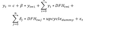
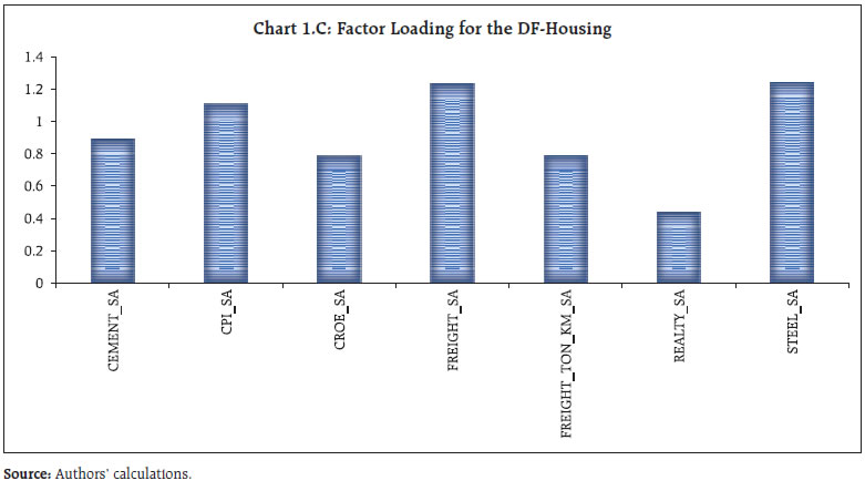
Source: Authors’ calculations. | III.2 Dynamic Factor for Realty Sector We attempt to use a data shrinkage technique to extract the common trend in the realty sector after selecting the relevant variables related to the realty sector. We start with each of the variables, i.e., steel and cement production, IIP core, rail-freight (also tonne per KMs), adjusted realty index, Google Search Propensity Index and housing prices- in their levels, de-seasonalised them using Census X-12, which are then z-score transformed for standardisation. Since we are attempting to capture one consensus underlying trend from several high-frequency indicators, differencing may lead to loss of information. This is consistent with the literature (Bhadury et al., 2020). The trend is obtained by estimating a dynamic factor model (DFM) using seven shortlisted variables. The procedure is in line with Stock & Watson (1989), which specifies an “unobserved single index” xt. The observation equation (yt=Zxt+α+vt) contains yt which is a n×1 matrix of economic indicators at a time t. The State specification (xt=Bxt-1+wt) extracts the common underlying trend in yt into a single-index dynamic factor. In this specification, Z represents factor loadings (Annexure Chart 1.C) and “α” refers to an offset factor. After estimating dynamic factor using the expected mean methodology4, we validate whether the DFH index tracks the housing development in India with an alternative data source, i.e., Proptiger, that reports the number of housing units sold across different cities. It appears that DFH is able to capture the broad trends that are observed in the housing market except during some policy intervention phases viz., housing for all, demonetisation, the introduction of RERA (Real Estate Regulatory Authority), etc. (Chart 2). Due to the limited observations of the city-wise data, we could not perform any in-depth empirical estimations; however, correlations of the respective city units sold and the DFH is in the range of 0.56 to 0.80 positive (2017-18 onwards), indicating that the DFH index is capturing the housing sector activities precisely. Next, we undertake a Granger Causality test among indicators of economic activities and DFH. The causality results indicate that there are evidences of one-way causation from the housing sector to economic activity. For brevity, we report the causality results in annexure (Table 1.B) and directly turn to the business cycle analysis, so that we can draw a few policy conclusions. For this, we use the same business cycle dating and create an upcycle dummy. We then regress lags of DFH and upcycle dummy using each of GVA, Non-Agricultural GVA, Non-Agricultural-Non- Construction GVA as our dependent variables. The regression equations could be summarised as an autoregressive equation of economic activities (GVA, and adjusted GVA) augmented by contemporaneous DFH, lagged DFH and upcycle interaction term. The equation is given as under: 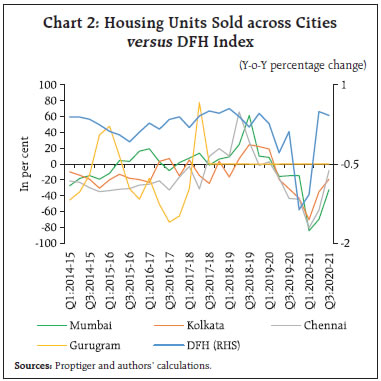
 DFH coefficients indicate a positive sign, which are statistically significant at the conventional levels for GVA and Non-Agri-GVA, when each of them is used as a dependent variable. Further, when an interactive dummy for an upcycle period was used in this regression, the coefficient of the interactive dummy turned out to be positive and significant, after a lag. The positive and significant value was consistent across all the dependent variables, which indicates the buoyancy of the realty sector growth during the upcycle period (Table 2). | Table 2: Regression Results | | Variable | GVA | GVA minus Agri | GVA minus Agri & Construction | | 1 | 2 | 3 | 4 | 5 | 6 | | | Coefficient | | C | 1.52 | 1.53 | 1.83 | 1.95 | 1.84 | 1.94 | | Dependent Variable lag | 0.73*** | 0.77*** | 0.71*** | 0.73*** | 0.71*** | 0.76*** | | DFH | 0.24* | 0.18 | 0.26* | 0.17 | 0.28 | | | DFH(-1) | | -0.98 | | -1.10 | | -1.15 | | DFH(-1) *UPCYCLE | | 1.02* | | 1.18* | | 1.22* | | R-Sq | 0.63 | 0.6 | 0.59 | 0.65 | 0.61 | 0.63 | | F-Stat | Significant at 1 per cent level | | N | 39 | Note: All variables are in y-o-y growth terms. The symbols *, **, *** denote the cases where we reject the null at the 10%, 5%, 1% significance levels, respectively. Based on the trimmed quarterly sample between 2010 and 2020.
Source: Authors’ calculations. | Construction is included in the GVA series; therefore, the above results could indicate both direct and indirect impacts. To identify the indirect impact, we exclude construction from Non-agricultural GVA (NANC-GVA) and use the same as dependent variable5. The positive and significant coefficients NANC-GVA capture the indirect impact of construction, that is positive and significant. It may be because of upstream and downstream linkages of the realty sector, which connects not only to capital-intensive sectors like cement and steel but also to several ancillary industries that are typically labour-intensive. III.3 Robustness of Dynamic Factor Housing Based on Table 1, we found six variables (including railways freight tonne per KM) having a high contemporaneous relationship while one is having a lagged relationship with GVA-construction. Though CPI housing prices indicated housing prices series is a lagged relationship, we believe that housing prices series is a very important variable and provide information about the housing market. However, from a technical point of view, housing prices could be considered separately. Therefore, we calculated DFH after removing the house price and found that our DFH_Houseprice is in line with our DFH. Similarly, notwithstanding the possibility of overlap, we considered both railway freight and railway freight tonne per KM, as we found their cyclical patterns are different (NDFH7). However, we computed DFH after excluding railways freight tonne per KM. The DFH_Freight_Tonne is reported in Chart 3. It indicates, except for a few time periods, the DFHs have been moving in tandem, tracking the broad trends in the Indian realty sector. IV. Conclusion Considering the importance of the realty sector for growth and employment generation, we attempt to evaluate its role in macroeconomic surveillance. While exploring the same for policy analyses, we discovered that the low data frequency (quarterly) and long lags in data availability have somewhat constrained the application of this sector in active policy making. In this article, we attempt to bridge this gap to facilitate faster information availability and policy analysis. In this vein, we examine various conventional monthly indicators, such as, housing prices, realty sector balance sheet, steel and cement production. We also look at unconventional indicators, such as Nifty Realty Index adjusted for broad market movements and Google search propensity indicator related to the real-estate sector. We then estimate a dynamic factor housing (DFH), to get a common factor from these variables that will capture the broad trend in the realty sector at a monthly frequency. Next, we validate that it indeed tracks the construction/realty sector, and therefore may be used for policy analysis. Our empirical findings indicate a positive and significant impact of DFH on GVA and non-agri-non-construction-GVA, indicating direct and second-round impacts of the realty sector on economic activities. We believe that the findings of this paper could be used in a variety of ways to improve policy analysis. To begin with, timely information facilitates efficient policymaking by minimising recognition lags. In this vein, the dynamic factor-based ‘DFH’ is likely to fill the void left by a monthly high-frequency variable capable of accessing the underlying situation and even aid in nowcasting construction GVA. Moreover, given the construction sector’s share in GVA, our findings regarding first and second-round effects indicate that the realty sector could play a significant role in the post-pandemic growth revival. References Ahmad, M., Zhao, Z. Y., & Li, H. (2019). Revealing stylized empirical interactions among construction sector, urbanization, energy consumption, economic growth and CO2 emissions in China. Science of the Total Environment, 657, 1085-1098. Berk, N., & Biçen, S. (2017). Causality between the construction sector and GDP growth in emerging countries: The case of Turkey. In 10th Annual International Conference on Mediterranean Studies (pp. 10-13). Bhadury, S., Ghosh, S., & Kumar, P. (2020). Nowcasting Indian GDP growth using a Dynamic Factor Model. RBI Working Papers No. 3 Government of India (GoI). (2013). The Economic Survey. ---.(2021). The Economic Survey. Hung, C. C., Hsu, S. C., Pratt, S., Chen, P. C., Lee, C. J., & Chan, A. P. (2019). Quantifying the linkages and leakages of construction activities in an open economy using multiregional input–output analysis. Journal of Management in Engineering, 35(1), 04018054. Kumar, A., & Chaudhary, N. (2014). Impact of Housing Investment on Indian Economy. International Journal of Languages, Education and Social Sciences. Mallick, H., & Mahalik, M. K. (2010). Constructing the economy: The role of construction sector in India’s growth. The Journal of Real Estate Finance and Economics, 40(3), 368-384. Ministry of Statistics & Programme Implementation (MOSPI). (2020). Estimates of Gross Domestic Product for the First Quarter (April-June) of 2020-21. Ramadorai, T. (2017). Report of the Household Finance Committee. Technical Report, Reserve Bank of India. Reserve Bank of India (RBI). (2020). Report on Trend and Progress of Banking in India. Stock, J., & Watson, M. (1989). New Indexes of Coincident and Leading Economic Indicators. Macroeconomics Annual, National Bureau of Economic Research, 4, 351-409. Tiwari, A. K. (2011). A causal analysis between construction flows and economic growth: evidence from India. Journal of International Business and Economy, 12(2), 27-42.
Annexure
| Table 1.A: Correlation of Selected Variables with Construction GVA (Pre COVID period) | | Variables | Construction GVA(-t) (Lagging Relationship) | Construction GVA (contemporaneous relationship) | Construction GVA(+t) (leading relationship) | Comments | | Housing credit | -0.0086 | -0.0676 | 0.1533 | No significant correlation | | Steel Production | 0.3392** | 0.3422** | -0.085 | C and L- | | Cement Production | 0.0681 | 0.5443** | 0.1715 | C | | IIP Core | 0.1817 | 0.2773 | 0.1491 | No significant correlation | | Housing prices | 0.3462** | 0.2344 | -0.0579 | L- | | Rail freight | 0.2015 | 0.28** | 0.1184 | C | | Rail_cement | -0.0101 | -0.1704 | 0.1567 | No significant correlation | | Realty Index | -0.098 | 0.2662 | 0.0644 | No significant correlation | | Sensex | -0.0392 | 0.11 | 0.096 | No significant correlation | | Adjusted Realty | -0.117 | 0.3153** | 0.025 | C | | Google Search Propensity Index | -0.1939 | -0.2101 | -0.022 | No significant correlation | Note: The symbols *, **, *** denote the cases where we reject the null at the 10%, 5%, 1% significance levels, respectively.
Source: Authors’ calculations. |
| Table 1.B Granger Causality Test | | Null Hypothesis: | Obs | F-Statistic | Prob. | | GDP does not Granger Cause DFH | 34 | 0.49 | 0.74 | | DFH does not Granger Cause GDP | | 1.70 | 0.17 | | NON_AGRI_GDP does not Granger Cause DFH | 34 | 0.33 | 0.85 | | DFH does not Granger Cause NON_AGRI_GDP | | 2.72 | 0.05 | | NON_AGRI_GDP_CONSTRUCTION does not Granger Cause DFH | 34 | 0.41 | 0.79 | | DFH does not Granger Cause NON_AGRI_GDP_CONSTRUCTION | | 2.05 | 0.10 | | Source: Authors’ calculations. |
|