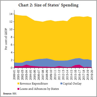
by Deba Prasad Rath, Bichitrananda Seth, Samir Ranjan Behera and Anoop K Suresh^{^}

This study investigates the relationship between States’ capital outlay and gross state domestic product (GSDP) while also identifying the factors that influence the States’ capital outlay decisions. An application of the panel framework for 15 Indian States revealed a positive and significant association between capital outlay and GSDP. Past capital outlay turns out to be a predictor of current capital outlay decisions and higher debt levels to be a barrier to public investment. States exhibit a counter-cyclical behaviour in terms of capital outlay under both negative and positive output gap environment. States may prioritize capital outlay while being cautious about higher debt levels, besides adhering to fiscal responsibility.

Introduction

As the world emerges from the COVID-19 pandemic, there is a growing consensus that governments’ capital expenditure could play a vital role in economic recovery (Berawi et al., 2020, Gaspar et al., 2020; OECD, 2021). Investing in infrastructure projects, renewable energy, and technology can create jobs, stimulate growth, and promote sustainability. Capital expenditure is a crucial tool used by governments to promote higher and stable economic growth particularly in economies that face infrastructural constraints (Ismail and Mahyideen, 2015; Waweru and Mose, 2021). India continues to be one of the fastest-growing economies in the world and maintaining high and sustainable growth would require significant investment in infrastructure. A recent estimate puts India’s investment requirement of US$840 billion over the next 15 years into urban infrastructure if it is to effectively meet the needs of its fast-growing urban population (World Bank, 2022). Recognising this, continued thrust has been provided to capital spending by the Centre and States in India, especially since the onset of the pandemic. For instance, capital expenditure by the Centre is budgeted to increase to 3.3 per cent of the GDP in 2023-24 from 2.7 per cent of the GDP in 2022-23 (RE). However, in a federal set up such as India, the sub-national governments’ capital expenditure decisions along with the central government, play a critical role in driving economic growth as well as promote social and economic development through investment in education, healthcare, and other social infrastructure. Moreover, capital expenditure by sub-national governments constitutes around two-third of the capital spending incurred by the General Government, while their own revenue is only one-third. Recently, State governments have increased their allocation towards capital spending, with capital outlay rising to 2.7 per cent of GDP in 2021-22 (from an average of 2.0 per cent in 2000s) and is budgeted to increase to an all-time high of 2.9 per cent in 2022-23. In this context, this article provides an assessment of the drivers of States’ capital outlay, as there is a paucity of empirical literature on this issue.

Apart from providing a set of stylised facts, thestudy utilises various data¹ analytic methods, such as panel cointegration, fully modified ordinary least square (FMOLS), and dynamic ordinary least square (DOLS), to assess the impact of capital outlay on gross state domestic product (GSDP). Thereafter, the study employs a two-way system generalised method of moments (GMM) to identify the factors influencing States’ decisions on capital spending, using the capital outlay to GSDP ratio as the dependent variable and factors such as one-year lagged debt-GSDP ratio, output gap, and dummy variables to capture the impact of election years and natural calamities as independent variables. Additionally, the study examines the asymmetric responses of States to debt levels and the output gap.

The rest of the article is divided into five sections. Section II undertakes a literature survey of past research studies in this arena. Stylised facts are outlined in Section III and provides essential insights into the research question. Section IV discusses the data and methodology employed in the study whereas the empirical results are presented in Section V. Lastly, Section VI concludes by outlining policy implications and recommendations based on the findings from our analysis.

II. Literature Review

The association between government’s capital expenditure and economic growth has led to a series of debates (Waweru and Mose, 2021). The capital expenditure incurred by the government has the ability to absorb new workforce, crowd in private investment and set the economy free from the vicious cycle of poverty (Leasiwal, 2021; Teklay, 2016; Victoria, 2015). Governments’ capital expenditure on human capital such as education and health further positively impact economic growth (Cullison, 1993; Paudel, 2023). On the contrary, it is also argued that the effect of capital expenditure on economic growth is negative attributable to the crowding out effect (Korman and Bratimasrene, 2007; Gregoriou and Ghosh, 2009).

In terms of determinants of capital expenditure by the government, budget constraints and debt levels have been considered as key factors influencing the government’s decisions on capital expenditure (Toubeau and Vampa, 2021; Idenyi et al., 2016; Lora and Olivera, 2007). Similarly, elections and natural calamities could affect their available budget for capital expenditure (Rasmussen, 2004; Rizqiyati and Setiawan, 2022).

In India, the multiplier effect of capital expenditure is found to be much higher at 7.6 than its revenue counterpart (Jain and Kumar, 2013). Furthermore, unlike the revenue expenditure multiplier, which has a short-run impact, the capital expenditure multiplier is dynamic, the effect of which lasts several years. Interestingly, capital expenditure is found to be particularly effective during periods of economic slack (RBI, 2022).

Overall, there are several studies that examine the association between government’s capital investment and economic growth; however, there seems to be a dearth of such studies at the sub-national level. Therefore, this paper attempts to contribute to the existing literature on the relationship between capital outlay and States’ GSDP for India and would aid in drawing implications for policy. These findings would enable the Indian States to make better decision and improve the medium to long-term economic growth prospective.

III. Stylized Facts

By convention, the expenditure incurred by the State governments are categorized into two distinct groups: revenue and capital. The former covers operational expenses such as salaries, wages, pension and supplies while the latter involves investment in infrastructure and other long-term assets. The capital expenditure is further subdivided into capital outlays as well as loans and advances which are provided to diverse entities by the States. We present a set of stylised facts that characterise the nature of major 15 States’ capital outlay in India.

Firstly, a significant portion of the States’ borrowing has been undertaken for capital outlay, unlike the initial years of the 2000s wherein they were utilised for meeting the revenue expenditure as evident from trends in ratio of revenue deficit to the gross fiscal deficit (RD-GFD) (Chart 1). A similar pattern is also visible for the revenue expenditure-capital outlay (RECO) ratio – another indicator of quality of expenditure. Although this ratio has risen since 2017-18, it is relatively smaller than its trend during the first half of the 2000s. Use of borrowings by States for capital outlay largely follows the principle that revenue deficits should be financed through revenue collection, and borrowings should be spent on creating productive assets so that the receipts emanating from the assets in the future can be used to repay the debt.

Secondly, the total expenditure of the States has been increasing since the fiscal year 2014-15. This increasing trend in expenditure could be attributed to factors such as the Ujjwal DISCOM Assurance Yojana (UDAY) scheme, farm loan waivers, and other development-related expenses. However, the growth of capital outlay has been relatively slow (Chart 2).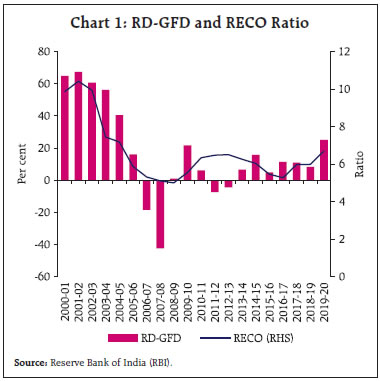

Thirdly, the capital outlay-to-GSDP ratio gradually increased from 1.3 per cent in 2002-03 to 2.5 per cent in the pre-global financial crisis (GFC) year driven by high growth in GSDP (Chart 3). With the slowdown on account of the impact of the GFC, States’ GFD increased above the fiscal responsibility legislation (FRL) limit, thereby reducing their capital outlay until 2010-11. Post 2013-14, however, this ratio recovered to 2.5 per cent by 2016-17 although it could not be sustained thereafter on account of increase in expenditure owing to factors noted above and revenue uncertainty due to the implementation of the goods and services tax (GST) regime from July 1, 2017.

Fourthly, State governments prioritise and allocate capital outlay towards various social and economic sectors. A significant proportion of the overall capital outlay is channelled towards the transport, irrigation, flood control, and energy sectors, while sectors related to human development, such as education and health, receive a comparatively smaller share (Chart 4). Barring education and health, this allocation pattern is consistent with the government’s emphasis on investing in infrastructure in order to promote economic growth and development.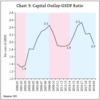

Fifthly, revised estimates (RE) tends to overshoot both budget estimates (BE) and actuals, with the most significant deviation arising from revenue receipts, mainly tax revenue (RBI, 2023). As a reaction, most States tend to reduce their allocation towards capital outlay in RE and further in actuals. Finally, as mentioned earlier, States are constrained by debt levels and economic conditions while deciding on capital outlay. Chart 5 illustrates that while capital outlay is inversely correlated with debt levels, it is positively correlated with GSDP growth.

In view of the stylised facts presented above, we now formally examine the relationship between capital outlay and economic growth at sub-national level as well as identify the role of various factors in determining States’ capital outlay.

IV. Data and Methodology

The study focuses on 15 Indian States.² As the first step of empirical analysis, the relationship between capital outlay and GSDP is investigated for 2000-01 to 2019-20. We use Pedroni and Kao’sresidual panel cointegration methods³, FMOLS, DOLS as our empirical approach. The data on capital outlay and GSDP were obtained from the Reserve Bank of India (RBI) and Ministry of Statistics and Programme Implementation (MoSPI), respectively. Stationarity tests confirmed that the variables in log form are non-stationary, i.e. I(1). Once the cointegration is established between capital outlay and States’ GSDP, the long-run coefficients are estimated.

In order to examine the determinants of States’ capital outlay, a two-way system GMM is employed in a panel setting. These methods allow for accounting endogeneity, individual-specific effects, and potential biases, providing consistent and reliable estimates. Here we use data on capital outlay for the same set of States for the period 2011-12 to 2019-20. We regress capital outlay to GSDP ratio on debt-GSDP ratio, outputgap⁴, natural calamity dummy, and election dummy. To attempt a further deep dive, the debt and output gap are provided an asymmetric treatment by including dummy variables separately for periods of high and low debt levels and interacting them withthe debt levels.⁵ Similarly dummies are also used for positive and negative output gap and interacted with the output gap variable.

V. Empirical Findings

Are Capital Outlay and GSDP cointegrated?

Pedroni residual cointegration tests indicates strong evidence of cointegration between the capital outlay and GSDP (Table 1). The Kao residual cointegration test, based on the augmented dickey fuller (ADF) test, also supported the presence of cointegration. Furthermore, employing a panel vector error correction model (VECM) ensured that theerror correction term⁶ is negative and statisticallysignificant.⁷

Table 2 presents the results of the two-panel regression models, FMOLS and DOLS, investigating the relationship between States’ capital outlay and GSDP and the coefficients turn out to be significant at 0.84 and 0.82, implying that a one per cent increase in States’ capital outlay is associated with a range of 0.82-0.84 per cent increase in GSDP.

What Factors Influence States’ Decision for Capital Outlay?

Next, we turn to the determinants of States’ capital outlay using two-way system GMM within a panel framework. As alluded to earlier, various factors, such as debt, economic conditions, natural disasters, and elections, impact the State’s decision to undertake capital outlay and our variables capture these dimensions.

(a) Baseline Results

Column (I) in Table 3 has baseline specification, while Columns (II) and (III) include an election year dummy and natural calamities dummy, respectively. The validity of the instruments (i.e., lags of debt-GSDP ratio) used in the study is assessed using the Hansen and Sargan tests. Both tests fail to reject the null hypothesis in all three equations, indicating that the model is correctly specified, and the instruments used are valid.

The coefficients of the lagged value of capital outlay to GSDP ratio have a positive and significant effect on all three specifications, suggesting that past values of capital outlay influence the current year’s decision. Furthermore, higher debt levels hinder a State’s ability to invest in capital outlay. As the debt-to-GSDP ratio has a negative coefficient in the equations, it indicates that States with more debt are less likely to increase their investment in capital outlay. The output gap has a negative effect on capital outlay, as shown by the statistically significant negative coefficients in column (II) and (III). An increase in the output gap leads to a decline in capital outlay. Both the dummy variables for elections and natural calamities are insignificant, implying that they do not significantly influence the States’ capital outlay decisions.

To capture the asymmetric response of States to debt levels (i.e., debt less than 25 per cent and more than 25 per cent) and economic conditions (i.e., positive and negative output gap), the base level equation (depicted in Column III of Tables 3 and Column I of Table 4) has been modified to the form depicted in Column II to V in Table 4. Aggregate debt variable is replaced by interacting dummies of debt less than 25 per cent (DL25) and more than 25 per cent (DM25), which are used alternatively in order to avoid dummy variable traps. Finally, alternative specifications for the output gaps, i.e., positive (POG) and negative (NOG) are also included in the system. All other variables are kept unchanged in all specifications.

Interestingly, the finding that States reduce public investment as the debt level increases cannot be generalized to all levels of debt. The insignificant coefficient of DL25 indicates that the State government’s decision to allocate capital outlay is not affected by a debt level lower than 25 per cent. This is attributed mainly to the fact that when the debt level is low, the State government has more financial flexibility to spend on public investment. On the other hand, the negative and statistically significant coefficient of DM25 suggests that when the debt level exceeds 25 per cent, the State government reduces its allocation of public investment. The State government faces financial constraints when the debt level is high, limiting its ability to spend on public investment. The higher debt level also increases the cost of borrowing, reducing the availability of funds for public investment.

The coefficient for output gap (OG) is negative and significant, both in positive and negative cases of output gap – a result which warrants careful interpretation. During positive output gap periods, it could be plausible that States commit to the path of fiscal consolidation i.e., to keep GFD-GSDP ratio within the FRL limit. During negative output gap periods, the Governments provide support to the economy through counter-cyclical fiscal policy. Part of this could also be in the form of higher capital expenditure. This policy has been evident in recent years as governments increased capital expenditure during the recovery period in the aftermath of the COVID-19 pandemic.

In summary, the study’s findings suggest that past values of capital outlay, debt-to-GSDP ratios, and economic conditions proxied by the output gap are significant factors influencing States’ capital outlay decisions. These findings have important implications for policymakers viz., investments in capital outlay may be hindered by high levels of debt highlighting the need for careful fiscal management and planning by the States.

VI. Conclusion

The empirical findings of the study revealed a significant and positive association between States’ capital outlay and GSDP - a one per cent increase in capital outlay leading to a range of 0.82-0.84 per cent increase in GSDP. Further, the findings also revealed that past values of capital outlay influence the current year’s decision, while higher levels of debt hinder States’ ability to invest in public investment. Additionally, State governments reduce their allocation of public investment when the debt levels are high. States exhibit a counter-cyclical behaviour in their allocation of capital outlay. The study’s findings provide important policy implications for State governments’ decision-making on capital outlay. While there is a need for prioritizing capital outlay due to their positive association with GSDP, adopting a prudent approach to public investment when debt levels are high is also called for. Thus, the analysis brings out the need for balancing the requirement for higher capital outlay with the goal of keeping the overall debt levels low and sustainable.

References

Berawi, M., Miraj, P and Sari, M (2020). Accelerating Infrastructure Development in Post-Pandemic Era. CSID Journal of Infrastructure Development. Vol. 3(114).

Cullison, W. E. (1993). Public Investment and Economic Growth. Federal Reserve Bank Of Richmond Economic Quarterly, 15.

Gaspar, V., Mauro, P., Pattillo, C and Espinoza, R (2020). Public Investment for the Recovery. IMF Blog. October.

Gregoriou, A and Ghosh, S. (2009). The Impact of Government Expenditure on Growth: Empirical Evidence from Heterogeneous Panel. Bulletin of Economic Research. Vol. 61(1). pp.95-102. February.

Idenyi, O.S., Ogonaa, I.C., and Ifeyinwa, A.C (2016). Public Debt and Public Expenditure in Nigeria: A Causality Analysis. Research Journal of Finance and Accounting.Vol. 7(10).

Ismail, N and Mahyideen, J. (2015). The Impact of Infrastructure on Trade and Economic Growth in Selected Economies in Asia. ADBI Working Paper Series. No.553. December.

Jain, R. and Kumar, P. (2013). Size of Government Expenditure Multipliers in India: A Structural VAR Analysis. RBI Working Paper Series. No.7. September.

Korman, J and Bratimasrene, T. (2007). The Relationship between Government Expenditure and Economic Growth in Thailand. Journal of Economic Education. Vol.14. pp. 234-246.

Leasiwal, T. (2021). Impact of Government Capital Expenditure on Poverty Levels in Maluku. Jurnal Cita Ekonomika, Vol.15(1). pp.43–49.

Lora, E and Olivera, M. (2007). Public Debt and Social Expenditure: Friends or Foes?. Emerging Markets Review. Elsevier, Vol. 8(4). pp. 299-310. December.

Organisation for Economic Cooperation and Development (2021). COVID-19 Transport Brief: Analysis, Facts and Figures for Transport’s Response to Corona Virus. March.

Paudel, R. (2023). Capital Expenditure and Economic Growth: A Disaggregated Analysis for Nepal. Cogent Economics and Finance. Vol. 11(1). March.

Rasmussen, T. (2004). Macroeconomic Implications of Natural Disasters in the Caribbean. IMF Working Paper. December.

Reserve Bank of India (2022). Report on Currency and Finance. April.

Reserve Bank of India (2023). State Finances: A Study of Budgets of 2022-23. January.

Rizqiyati, C and Setiawan, D. (2022). Do Regional Heads Utilize Capital Expenditures, Grants, and Social Assistance in the Context of Elections? Economies. Vol.10(220). September.

Teklay, B. (2016). Impact of Government Capital Expenditure on Growth of Private Sector Investment: The Case of Ethiopia. Developing Country Studies. Vol. 6(4). pp.49-61.

Toubeau, S and Vampa, D (2021). Adjusting to Austerity: The Public Spending Responses of Regional Governments to the Budget Constraint in Spain and Italy. Journal of Public Policy, Cambridge University Press. Vol. 41(3). pp. 462-488. September.

Victoria, J (2015). Human Capital Investment and Economic Growth in Nigeria. African Research Review. 9(1). S/No. 36. January.

Waweru, D and Mose, N. (2021). Government Capital Expenditure and Economic Growth: An Empirical Investigation. Asian Journal of Economics, Business and Accounting. Vol.21(8). pp.29-36. June

World Bank (2022). Financing India’s Urban Infrastructure Needs: Constraints to Commercial Financing and Prospects for Policy Action. November.

^{^} The authors are from the Department of Economic and Policy Research. The authors are thankful to Dr. G.V. Nadhanael for his valuable inputs and suggestions. The views expressed in this article are those of the authors and do not necessarily represent the views of the Reserve Bank of India.

¹ For examining relationship between States’ capital outlay and their GSDP, we have utilised a panel dataset from 15 major Indian States spanning 20 years from 2000-01 to 2019-20. The study deliberately does not extend to 2022-23, as it may have been influenced by abnormal factors that could have skewed the results. On the other hand, for examining the factors determining States’ capital outlay, we have confined the period of analysis from 2011-12 to 2019-20.

² Andhra Pradesh (including Telangana), Bihar, Gujarat, Haryana, Jharkhand, Karnataka, Kerala, Madhya Pradesh, Maharashtra, Odisha, Punjab, Rajasthan, Tamil Nadu, Uttar Pradesh, and West Bengal.

³ The Pedroni test assumes cross-sectional independence in the residuals, while the Kao test allows for cross-sectional dependence by modelling a common factor in the residuals. Moreover, the Pedroni test allows for heterogeneity in the intercept and trend coefficients across cross-sections, whereas the Kao test assumes homogeneity of the cointegration relationship across cross-sections.

⁴ Output gap is estimated using HP filter.

⁵ These dummy variables take the value of 1 for periods when the actual debt levels are in the top or bottom quartile (25 per cent). The threshold of debt-GSDP ratio at 25 per cent is chosen based on the average of the ratios from 2015-16 to 2019-20 of all States. This ratio, however, does not represent an optimal level of debt or sustainable level of debt.

⁶ The error correction term represents the short-run dynamics between the variables, indicating how quickly the variables adjust to deviations from the long-run equilibrium relationship. If the coefficient of the error correction term is negative and statistically significant, it indicates that deviations from the long-run equilibrium are corrected in the short run, meaning that if capital outlay deviates from its long-run equilibrium level, it would adjust to that level in the short run.

⁷ Results of panel VECM are not presented in the paper. However, they would be made available upon request.