by Michael Debabrata Patra, Joice John and Asish Thomas George^ Examining properties such as persistence, anchoring, generalisation, convergence and cyclical sensitivity, this article finds that supply shocks during 2020-22 transited the Indian economy to a high inflation regime. Since the second half of 2022-23, there is a rising probability that inflation is transiting away from the high regime with a decline in persistence and trend, even as it is exhibiting increasing sensitivity to demand factors. The task of monetary policy is to guide the economy to a low inflation regime while being in readiness to address the rising sensitivity of inflation to demand pull. In India, inflation declined from double digits in the early 2010s and aligned with the legislatively mandated target of 4 per cent set under the flexible inflation targeting (FIT) framework over the period 2016 to 2019. The onset of the Covid-19 pandemic brought in lockdowns, massive urban-to-rural migrations and severe supply disruptions. Just as signs of waves of the pandemic abating become evident, the war in Ukraine since February 2022 reignited inflationary pressures catching central banks across the globe wrong footed by what seemed to be multiple supply shocks (supply chain disruptions; container shortages; port and shipping dislocations; war-induced evaporation of food, energy, fertilisers and metal supplies; sanctions and financial fragmentations) when incipiently a surge in pandemic-liberated demand was taking hold as it rotated away from contact-intensive services. Quickly inflation became global, stinging central banks into the most aggressive and synchronised monetary policy response in several decades. In India, inflation remained above the upper tolerance band, triggering statutory accountability procedures by November 2022. This article peers underneath the inflation prints to try to decipher why India was ambushed by these inflation regime shifts - the high inflation experience of 2020 and 2022, followed by signs of transition. It follows influential work on a two-regime view of inflation with focus on transitions (Borio, et al., 2023) to analyse the properties of those regimes in India after statistically identifying them in section II. We examine the behaviour of trend inflation, its persistence and stochastic volatility in order to examine the state of inflation expectations. Externalities associated with these regime changes in inflationary pressures, their generalisation tendencies and relative price dynamics are parsed in section III with a view to understanding the broad-based nature of inflation. Section IV revisits the convergence properties between core and headline so as to examine the durability of inflationary pressures. Section V investigates the cyclical sensitivity of inflation across regimes to evaluate the role of demand factors in the evolution of inflation. Section VI concludes with some policy perspectives. II. Regime Shifts in India’s Inflation History The Markov switching model (Hamilton,1989) is among the most popular nonlinear time series regime switching models in the literature. This model examines multiple structures that can depict inflation behaviour in different regimes, characterising the complex dynamic patterns switching between these structures. A Markov switching model applied on year-on-year (y-o-y) inflation rates in India from January 2012 to March 2023 reveals that with the de facto introduction of FIT in India in 2014, inflation shifted from a high regime in which it averaged over 8 per cent during 2012-14 to a lower regime averaging 4.4 per cent. With the outbreak of the Covid-19 pandemic in early 2020, inflation moved back to a high regime for a brief period. As the pandemic seemed to abate, inflation reverted to a low regime by early 2021 and remained there till the Ukraine war in early 2022 caused it to move back to a high regime during the first half of 2022-23. Since H2 of 2022-23 there is a rising probability that inflation is transiting away from the high regime (Chart 1). 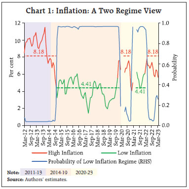 In line with the seminal work on the subject (Stock and Watson, 2007 and Cogley, et al., 2010), we decompose inflation into two components – trend and cycle. Changes in the trend component are highly persistent, whereas shocks to the cyclical component are temporary. Equations (1) and (2) are estimated as time-varying parameter regressions with stochastic volatility (TVP-SV) wherein inflation is measured by seasonally adjusted month-on-month (m-o-m) annualised rate of the Consumer Price Index (CPI). We observe that the “intrinsic” element, which represents the persistence of inflation due to its own past or price-setting inertia, was high during 2011-13. It declined from 2014 and remained low through 2016 till 2019. After the Covid-19 shock in early 2020, inflation persistence started to increase till it peaked in April 2022. More recently, intrinsic inflation persistence seems to be on a declining trajectory (Chart 2). Equations (1) and (2) can also be utilised to filter out the unobserved trend in inflation in India. Trend inflation in India fell down from the peak during 2011-13 and remained range bound around the target during 2016-19. It started to increase after the onset of the pandemic, i.e. from early 2020, but it is found to be very gradually returning to the target (Chart 3). 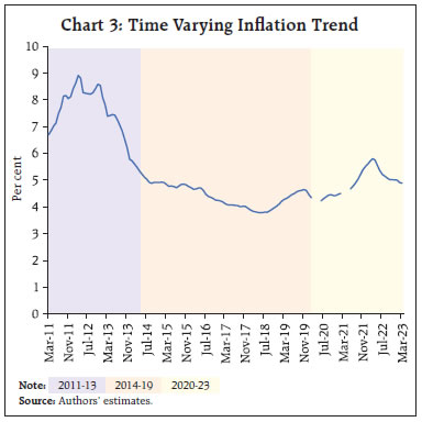 Decomposing the variability in inflation into trend and cyclical components shows a marked increase in both components, post Covid-19 period. Overall, in all regimes inflation variability has been mainly driven by its cyclical component, indicating the role of supply shocks. The variability of the trend component of inflation, has declined from its highs during 2011-13 and remained modest till 2019, indicating that inflation expectations were getting anchored. After the Covid-19 shock, however, volatility in the cyclical component of inflation caused by supply also translated into an increase in the variability of trend inflation suggesting de-anchoring of inflation expectations (Chart 4). III. Relative Price Dynamics and Inflation Spillovers Has the inflationary process been driven by relative prices or is it generalised? Without spillovers, commodity-specific price increases will die out over time rather than getting generalised. Even when commodity prices exhibit volatility, idiosyncratic changes independent of each other will get reflected in relative price changes rather than becoming broad-based. We measure the spillovers of price changes across different constituent sub-groups of the CPI by using the generalised forecast error variance decomposition (GFEVD) over a given horizon (say 12 months) as estimated from a Vector Auto Regression (VAR) of sub-group level m-o-m annualised inflation (Borio, et al., 2023). Off-diagonal elements of GFEVD matrix represent the shares of variance in inflation of each sub-group that is explained by inflation in other sub-groups. A measure of total spillovers can be constructed by a weighted aggregate of the off-diagonal elements of the GFEVD matrix. It represents the amount of variance in inflation pertaining to each sub-group, which is not explained by its own shocks, but instead by the transmission of shocks from other sub-groups inflation working through the lag structure of the VAR (Borio, et al., 2023). It is depicted in a heat map (Chart 5). Darker shades of red indicate greater spillovers from sub-groups on the horizontal axis to the sub-groups on the vertical axis. The diagonal elements of the matrices in Chart 5 represent own shocks and do not contribute to spillovers across sub-groups. The weighted sum of all the off-diagonal elements of the GFEVD matrix in the second sub-sample (2014-19) is 45 per cent, which is substantially lower than that of the first sub-sample (2011-13, 60 per cent). Post-2020, there is an increase in spillovers captured by the shading becoming darker – the average weighted spillover stood at 74 per cent during this period. 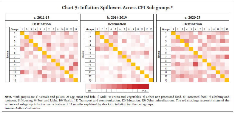 Another approach to measure the inflation spillovers is to decompose the cross-sectional variance of 12 month inflation into the portion attributable to two components: a) the aggregate weighted variance of inflation in sub-groups and b) the aggregate covariances between them, the latter being an indicator of inflation spillovers across sub-groups (Borio, et al., 2023). This decomposition shows a decline in overall variance in inflation during 2016-19 on account of reduced covariances in inflation among sub-groups and hence lower degree of their co-movement and anchoring. Total variance in inflation, its variances in sub-groups and covariance has increased after 2020, the latter pointing to generalisation of inflation. Hearteningly, total variance in inflation has shown a decline since October 2022 on account of a decline in covariance, however, individual sub-groups are exhibiting higher inflation volatility, which are idiosyncratic and independent of each other (Chart 6). In more recent months, therefore, inflation generalisation is getting weaker and it is localised price movements that are driving the inflation. IV. Headline-Core Convergence The underlying or core inflation rate filters out transitory fluctuations in headline inflation and provides a stable underlying measure of inflation that is free of the effects of sectoral shocks. Since volatility can also emerge from price changes in CPI sub-groups other than food and fuel, “outlier-exclusion” measures of core inflation have become popular (Ball, et al., 2023). The simplest type is the weighted median inflation in which 50 percent of the distribution of CPI item-level inflation rates is trimmed off on each side and core inflation is measured by the inflation rate in the middle. Two different types of weighted median measures of core inflation are constructed. For each month a measure of median inflation is computed over the previous 12 months. This is done by computing each CPI item’s inflation rate from month t-12 to month t and taking the weighted median. The weighted median inflation can be defined at time t by considering all CPI items under a ranking operator, which ranks item-specific inflation rates from smallest to largest and cumulates their corresponding weights. The weighted median inflation rate is selected as the inflation rate at time t for the CPI-item at which the sum of the ranked weights is at above the 50th percentile (Ball and Mazumder, 2019). The weighted median can become a biased estimator of core inflation that its average over time is lower than that of headline inflation. A bias adjusted measure is defined as the inflation rate at that percentile of the item-level inflations with the smallest average difference between its value and that of headline inflation (Ball, et al., 2023). The bias adjustment is dependent on the sample period. Here, we have adjusted the bias in the sample for the period January 2015 to March 2023 so that headline and core inflation have almost the same mean during that period. Weighted median inflation (y-o-y) shows persistence (Chart 7a). The bias adjustment pushes core inflation further up (Chart 7b). In contrast to the y-o-y measure, the m-o-m weighted median shows a decline since the Ukraine war related inflation spike in Q1:2022-23, indicating that the y-o-y weighted median inflation may also decline further going forward in the absence of any unfavourable shocks (Chart 8a, b). One way to check whether item-level price changes are likely to have significant consequences for underlying inflation is to investigate whether headline inflation tends to converge to core or vice versa. When headline converges to core volatile price changes incline to dissipate, by contrast, when core converges to headline, those price changes indicate potentially powerful second-round effects (Cecchetti and Moessner, 2008; Borio, et al., 2023). To examine this proposition, we estimate the following two regression equations allowing parameters to change over time:
V. Role of Demand and Supply By making use of historically determined weights based on correlations between sub-group level inflation and a measure of aggregate demand proxied by output gap (Patra, et al., 2021), cyclically sensitive inflation can be estimated (Stock and Watson, 2020; Patra, et al. 2022). There could be various explanations as to why the sensitivity of inflation to economic activity might differ from one sub-group to another. First, the cyclical sensitivity of the price of a good or service depends whether it is set on international or domestic market conditions. For example, with around 85 per cent of fossil fuel demand met through imports, India is typically a taker of prices set in global markets. Hence the link between domestic demand and the transportation costs will be influenced by import prices of crude oil. On the other hand, CPI categories such as household goods and services, education and housing have prices that are based on local market conditions and subject to domestic cyclical movements. In general, price-setting behaviour differs across sub-groups based on market structure, wage-setting process and other structural factors. Second, measurement issues also contribute to differences in sensitivity to inflation. Accordingly, Cyclically Sensitive Inflation (CySI) is computed for India to identify which parts of the CPI are impacted by economic cycles (demand). The weights attached to each part is extracted from time varying Phillips curves estimated at the sub-group level (Patra, et al., 2022). The results show that CySI has contributed substantially to the pre-2014 high inflation regime. Since the de facto adoption of the FIT in India in 2014, the contribution of CySI has declined. During the pandemic period (since Q1 of 2020), CySI remained persistently lower than acyclical inflation, indicating the collapse of demand (Patra et al., 2022). Thus, it were acylcial factors induced by supply bottlenecks and lockdowns that instead drove headline inflation. Since H2 of 2022-23 the contribution of CySI has been rising (Chart 10) and the gap between the acyclical inflation and CySI has turned negative, signalling the appropriateness of monetary policy action (Patra et al., 2022). 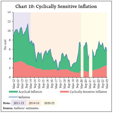 Global factors played a large role in the transition of inflation to a high regime since H2 of 2020-21 till H1 of 2022-23; in contrast, domestic factors were dominant in the earlier high inflation regime prior to 2014. From the second half of 2022-23, the contribution of imported inflation had been gradually declining and domestic factors were playing a larger role, reflecting the increasing role of cyclically sensitive inflation.1 VI. Conclusion Over the decade gone by, inflation in India has switched from a high pre-FIT regime to a low FIT regime and back under unprecedented and overlapping shocks. Since the second half of 2022-23, there are signs of a transition to a low inflation regime. Our findings can be summarised into two parts. First, it was the succession of supply shocks during 2020-22 that transited the Indian economy to a high inflation regime. Our measure of cyclically sensitive inflation remained persistently lower than the acyclical inflation even after the incidence of the shocks, indicating the absence of demand pull in the transition to the new regime. In the transition, inflation exhibited persistence and an upshift in its trend. Alongside, the volatility of both trend and cyclical components surged. Taken together, these results point to inflation expectations breaking loose from the anchoring that had occurred during 2016-19. The clear vision of hindsight would show that monetary policy action was warranted to restore credibility and re-anchor expectations, justifying the effective increase of 3.2 percentage points in the weighted average call money rate, the operating target of monetary policy in India, between March 2022 and March 2023. Influential work on a two-regime view of global inflation cited earlier highlights the importance of monetary policy being pre-emptive when the risk of a transition to a high inflation regime increases, although it acknowledges the challenge of assessing this risk in real time (Borio, et al., 2023). Delaying the response will warrant more forceful actions inevitably, with implications for the sacrifice of growth. The supply shocks of 2020-22 increased the total variance of headline CPI inflation as well as covariance among inflation in its sub-groups. This translates to evidence that in the high inflation regime, there has been a generalisation of price pressures – they have spread across many sub-groups, which are experiencing more co-movement of high inflation than normally seen. This is a clearer call for monetary policy action to quell inflationary pressures and contain their broad-basing. Again, the monetary policy actions and stance of the Reserve Bank through 2022-23 are validated. Second, what do our findings suggest for the way forward? In terms of the regime shift exercise, there is a rising probability since the second half of 2022-23 that the Indian economy is transiting away from the high regime. Absent unfavourable idiosyncratic shocks, conditions are right for early signs of grudging disinflation to firm up into a central tendency. Also, inflation persistence and trend are on the decline, however gradual, suggesting that inflation expectations are slowly getting re-anchored as policy actions and stance are gaining traction and have started showing demand restraining influences. For monetary policy, the recommendation would be: wait and watch, while guiding inflation towards the imminent onset of a low inflation regime. Since the second half of 2022-23, individual sub-groups are exhibiting higher volatility – sporadic supply shocks are at work – but, importantly, covariance is declining. This suggest that generalisation or broad-basing of inflationary pressures is on the ebb and increasingly localised price movements are influencing headline inflation. This calls for fine-tuning measures to align demand and supply of specific goods and services, which lies outside the realm of monetary policy but are being undertaken on an ongoing basis to head off potential price pressures from getting deep-seated. Additional evidence that inflationary pressures in India are easing is found in the decline in the m-o-m momentum of core inflation, reinforcing empirical support for a low inflation regime ahead of us from the proposition that headline inflation will inevitably converge to its core. A dissonant note in our findings is that our cyclically sensitive inflation measure is increasing. This indicates that demand pull is increasingly gaining traction. For monetary policy, therefore, there can be not letting down of the guard. Readiness to act pre-emptively to ensure that the disinflation that is underway is not interrupted is our policy recommendation for the way forward. References Ball, L. M., & Mazumder, S. (2019). The nonpuzzling behavior of median inflation (No. w25512). National Bureau of Economic Research. Ball, L. M., Carvalho, C., Evans, C., & Ricci, L. A. (2023). Weighted median inflation around the world: A measure of core inflation. IMF Working Papers, 2023 (044). Borio, C., Lombardi, M., Yetman, J., & Zakrajšek, E. (2023). The two-regime view of inflation. BIS Papers. Cecchetti, S. G., & Moessner, R. (2008). Commodity prices and inflation dynamics. BIS Quarterly Review, 55-66. Cogley, T., Primiceri, G. E., & Sargent, T. J. (2010). Inflation-gap persistence in the US. American Economic Journal: Macroeconomics, 2(1), 43-69. Hamilton, J. D. (1989). A new approach to the economic analysis of nonstationary time series and the business cycle. Econometrica: Journal of the econometric society, 357-384. Nakajima, J. (2011). Time-varying parameter VAR model with stochastic volatility: An overview of methodology and empirical applications. Patra, M. D., Behera, H., & John, J. (2021). Is the Phillips Curve in India dead, inert and stirring to life or alive and well? RBI Bulletin November. Patra, M. D., George, A. T., Nadhanael, G. V., & John, J. (2022). Anatomy of inflation’s ascent in India. RBI Bulletin December. Stock, J. H., & Watson, M. W. (2007). Why has US inflation become harder to forecast?. Journal of Money, Credit and banking, 39, 3-33. Stock, J. H., & Watson, M. W. (2020). Slack and cyclically sensitive inflation. Journal of Money, Credit and Banking, 52(S2), 393-428.
|