by Abhilasha#, Bhimappa Arjun Talwar^, Krishna Mohan Kushwaha^ and Indranil Bhattacharyya^ Open market operation (OMO) is a major liquidity management instrument of central banks in a modern market-based monetary policy framework. In India, OMOs have gained prominence in the toolkit of the Reserve Bank of India (RBI) over the last decade. In this context, this article provides an overview of the conduct of OMOs and its implications for the RBI’s balance sheet. An empirical assessment demonstrates the significant impact of key domestic and global factors on 10-year G-sec yields. Introduction Open market operation (OMO) is the process by which the central bank purchases (sells) government securities (G-secs) or other financial assets from (to) banks and financial institutions. In a modern market-based financial system, central banks use OMOs as one of the tools for implementing monetary policy. Generally, OMOs are conducted to adjust the supply of primary liquidity (base money) in an economy, thus influencing total money stock. The advantage of OMOs is that they can be flexibly used by the central bank and are easily reversible, thus considerably reducing the lags of monetary policy (Mishkin, 1997). Moreover, OMOs fit seamlessly into all monetary policy frameworks spanning inflation targeting, monetary targeting, currency boards, and exchange rate targeting. While OMOs figured prominently in the arsenal of central banks in advanced economies (AEs) for nearly a century (Vlieghe, 2020), they have gradually gained importance in emerging market economies (EMEs) with the development of markets and the proliferation of instruments. With several countries undertaking large scale asset purchases – mainly of government bonds – in the aftermath of the global financial crisis (GFC) and the COVID-19 pandemic, OMOs are at the center stage of policy making. The remark by a US Federal Open Market Committee (FOMC) member underscores this recognition – “we are running more open market operations, for greater sums, than at any time in our history” (Williams, 2020). Central bank purchases of G-secs through OMOs augment systemic liquidity by increasing the reserves of commercial banks thereby enabling the latter to expand their loan and investment portfolios. This can, inter alia, increase the price of G-secs with concomitant reduction in their yields; and facilitate reduction in the interest rates of financial instruments that are priced off the risk-free rate, i.e., G-sec yield, thereby stimulating economic activity. The impact is opposite in the case of sale of G-secs by the central bank. Thus, OMOs provide greater flexibility to central banks in conducting monetary policy through the market mechanism – the discretion to determine the timing and volume of monetary operations – rather than resorting to direct controls to regulate systemic liquidity (Axilrod, 1997). More recently, the Bank of England undertook temporary purchase of long-dated government bonds worth £19.3 billion for a limited period on financial stability considerations. In EMEs such as India, OMOs also serve the additional purpose of sterilising the monetary impact of large capital inflows arising out of global policy spillovers (Raj et al., 2018). In the Indian context, OMOs emerged as a key instrument with the progressive liberalisation of the economy and reforms in the G-sec market viz., the introduction of auctions and the shift towards market-based pricing of G-secs. In this regard, OMOs – both outright and reversible transactions – were conducted frequently, particularly with the introduction of the liquidity adjustment facility (LAF) in June 2000. Against the backdrop of India’s increasing integration with global financial markets, OMOs gained additional prominence in sterilising the liquidity impact of large capital inflows, which surged on account of search for yields and policy spillovers from AE central banks. Moreover, OMOs were also used to calibrate systemic liquidity1 in sync with the monetary policy stance and were used extensively to inject durable liquidity2 when systemic liquidity was in deficit. Thus, OMOs gradually supplanted the cash reserve ratio (CRR) as a flexible tool for management of durable liquidity. Furthermore, OMOs can assuage market sentiments and facilitate the orderly evolution of the yield curve, which is deemed as a public good (RBI, 2020). This objective was, for example, met through the (i) introduction in December 2019 of special OMOs – the simultaneous purchase and sale of G-secs – commonly referred as operation twist (OT); and (ii) the announcement of the secondary market government securities acquisition programme (G-SAP) in April 2021. In India, the spotlight has been on OMOs since the beginning of the last decade and especially after the introduction of flexible inflation targeting (FIT). OMOs emerged as a major tool of liquidity management even prior to the pandemic; for example in 2018-19, the RBI resorted to large scale OMO purchases to inject liquidity. Given the versatility of its use in recent years in a market-based monetary policy framework and especially after the outbreak of COVID-19, this article examines the key drivers, both global and domestic (including the conduct of OMO auctions), that have a bearing on 10-year G-sec yields. Specifically, this article focuses on outright OMOs which have a durable liquidity impact rather than the reversible transactions which are undertaken mainly to address transient liquidity variations. In this backdrop, the remaining part of the article is structured in the following manner. Section II presents a stylised view of OMOs and its variants while Section III provides an overview of the conduct of OMOs in India and its implications for the Reserve Bank of India (RBI)’s balance sheet. An empirical scrutiny of the various drivers of 10-year G-sec yields in India is taken up in Section IV while Section V concludes. II. Open Market Operation and its Variants As mentioned earlier, OMOs entail purchase (sale) of securities leading to injection (absorption) of liquidity to (from) the banking system. OMO is an umbrella term for various kinds of central bank operations – repo or reverse repo operations; outright purchase/sale of G-secs issued by the government or the central bank’s own bills; and forex operations/swaps – which impact the supply of reserves in the system. Most central banks classify repurchase operations, which are transient in nature, also as OMOs. In India, however, outright purchase or sale of G-secs resulting in injection/absorption of durable liquidity are classified as OMOs while temporary liquidity movements are managed through repurchase transactions conducted under the LAF. Central banks generally adjust the supply of money through OMOs to steer short-term interest rates which, in turn, influence longer-term rates and overall economic activity. Following the GFC, central banks in AEs eased monetary policy by reducing interest rates until short-term rates reached the effective lower bound (ELB) – close to zero – which constrained further rate reductions thereby limiting conventional monetary policy options. To circumvent the ELB problem, unconventional monetary policies (UMPs) were deployed on a large scale, including purchase of long-term bonds to further reduce long-term rates and ease monetary conditions. Central banks had undertaken large scale OMO purchases after the GFC and especially in response to COVID-19, to both inject liquidity and lower long-term yields, given the ELB constraint. Specifically, OMOs reduce yield through the supply channel – an OMO announcement can immediately moderate the risk premium in anticipation of reduced net supply of government bonds in the market (Arora et al., 2021). While a quantity target of OMO purchases (or other risky assets) is coined as quantitative easing (QE), a price target is known as yield curve control (YCC). Under QE, large scale purchases reduce yields thereby lowering longer-term rates and easing financial conditions. In case of YCC, the target price becomes the market price once the bond markets internalise the central bank’s commitment to buying any amount (BIS, 2019); i.e., the central bank continues to purchase bonds till bond prices stabilise at the target price. Therefore, both QE and YCC can potentially lead to unbridled expansion in the central bank’s balance sheet While the US Federal Reserve (Fed) undertook large scale QE after the GFC, the Bank of Japan (BoJ) adopted YCC3 in 2016 to peg yields on 10-year Japanese government bonds (JGBs) around zero to combat persistent deflation risks4. This has been categorised as quantitative and qualitative monetary easing – a policy by which the BoJ signals its strong commitment to price stability while purchasing massive amounts of JGBs, including bonds with longer residual maturities to actively influence expectation formation of private entities (Kuroda, 2016). OT is a variant of QE used by the Fed in 1961 and more recently in 2012. The “twist” in the operation occurs when the central bank uses sale proceeds of short-term treasury bills to buy long-term treasury notes, which lowers longer-term interest rates thereby reducing the term premium (Bernanke, 2020). OTs, thus, are usually liquidity neutral – purchases in select maturity segments are nullified through sales of other maturities of an identical amount. While OMO purchases lower the level of yields across the term structure, OTs alter the slope of the yield curve through targeted intervention at specific maturities (Patra and Bhattacharyya, 2022). Even as OMOs are integral to the toolkit of central banks globally, there are key differences in modalities (Annex Table 1). III. Open Market Operations – The Indian Experience The RBI has been conducting OMOs since its inception in 1935, but those operations were mainly undertaken in pound sterling. The RBI Annual Report of 1948 mentioned OMO purchase of G-secs for the first time; thereafter, a few years later, sharp movements in money supply were attributed to OMO purchases of G-secs. By the 1980s, the efficacy of OMOs, however, as a monetary policy instrument was blunted (Das, 2020), due to (i) an underdeveloped G-secs market; (ii) a system of administered rates; (iii) a captive investor base (banks) for G-secs ensured through periodic hikes in the statutory liquidity ratio (SLR); and (iv) deficit financing induced surplus liquidity conditions which reduced banks’ reliance on central bank funding. Post the initiation of economic reforms, the government borrowing programme was conducted through auctions for the first time in 1992. Moreover, the automatic monetisation of fiscal deficit came to an end in 1997 as the RBI terminated the practice of issuing ad hoc Treasury bills (T-bills). The SLR was also reduced to the then prevailing floor of 25 per cent of net demand and time liabilities (NDTL) in October 1997 and, thereafter, continued to be reduced gradually. From the second half of the 1990s to 2003-04, the RBI took frequent recourse to OMO sales to modulate the liquidity impact of capital inflows. Consequent to the enactment of the Fiscal Responsibility and Budget Management (FRBM) Act, 2003, RBI’s withdrawal from the primary market for G-secs in 2006 also facilitated the emergence of OMOs as a key tool for monetary management5. When the GFC flared up in 2008, the RBI, inter alia, undertook large scale OMO purchases to offset capital outflows triggered by financial market panic and “flight to safety”. The RBI issued an indicative calendar for OMOs in 2009-10 to address the liquidity requirements of the economy. During the last decade, RBI conducted two-way OMOs extensively to inject (absorb) durable liquidity (Table 1). In April 2016, the liquidity management framework was revised in a move to progressively lower the average ex ante liquidity deficit to a position closer to neutrality6. The RBI assured the market of meeting durable liquidity requirements; accordingly, liquidity injections through OMO purchases more than offset the liquidity drainage due to currency leakage and FCNR(B) redemptions during 2016-17. With the introduction of FIT in the same year, OMOs – more purchases than sales – remained a key instrument for liquidity management. After demonetisation, cash management bills (CMBs) were issued under the market stabilisation scheme (MSS) for a limited period to absorb surplus liquidity. Anticipating that the liquidity hangover from demonetisation may persist through 2017-18, the RBI provided liquidity guidance in April 2017 with a view to moderating systemic liquidity towards neutrality, which included inter alia the conduct of OMOs to manage durable liquidity. OMO purchases amounted to ₹2.99 lakh crore during 2018-19 – to infuse durable liquidity and manage the enduring liquidity impact of forex interventions. | Table 1: Open Market Operations | | (₹ crore) | | | Auction | NDS-OM | Total | | Purchase | Sale | Net Purchase | Purchase | Sale | Net Purchase | Purchase | Sale | Net Purchase | | 2013-14 | 54,535 | 2,532 | 52,003 | 44 | 45 | -1 | 54,579 | 2,577 | 52,002 | | 2014-15 | 0 | 29,268 | -29,268 | 10 | 34,160 | -34,150 | 10 | 63,428 | -63,418 | | 2015-16 | 71,409 | 8,270 | 63,139 | 16,715 | 27,530 | -10,815 | 88,124 | 35,800 | 52,324 | | 2016-17 | 1,10,014 | 0 | 1,10,014 | 500 | 20 | 480 | 1,10,514 | 20 | 1,10,494 | | 2017-18 | 0 | 90,000 | -90,000 | 1,235 | 10 | 1,225 | 1,235 | 90,010 | -88,775 | | 2018-19 | 2,98,502 | 0 | 2,98,502 | 780 | 50 | 730 | 2,99,282 | 50 | 2,99,232 | | 2019-20* | 1,32,500 | 28,276 | 1,04,224 | 13,190 | 3,845 | 9,345 | 1,45,690 | 32,121 | 1,13,569 | | 2020-21* | 3,02,132 | 1,90,545 | 1,11,587 | 2,05,588 | 3,880 | 2,01,708 | 5,07,720 | 1,94,425 | 3,13,295 | | 2021-22** | 2,30,000 | 40,000 | 1,90,000 | 48,061 | 24,085 | 23,976 | 2,78,061 | 64,085 | 2,13,976 | *: Includes OT.
**: Includes OT and purchases under G-SAP.
Source: RBI. | Besides injecting liquidity through OMOs amounting to ₹1.13 lakh crore during 2019-20, the RBI announced special OMOs – involving the simultaneous purchase of long-term and sale of short-term securities – or “operation twist” in December 20197, predating the COVID-19 outbreak in India. These operations aimed at compressing the term premia thereby reducing the slope (steepness) of the yield curve and distributing liquidity more evenly across the term structure8. Moderation in the long-term G-sec rates, in turn, got reflected in other financial market instruments that are priced off the G-sec rate, thereby improving monetary transmission. Up to August 2022, the RBI conducted 26 such operations which were generally liquidity neutral, i.e., purchases offset through sales of identical amount9 (Annex Table 2). In the wake of the pandemic, the RBI unveiled a slew of conventional and unconventional measures to stimulate market activity, ease funding cost and improve monetary transmission. OMOs figured prominently in this strategy with an unprecedented net purchase of ₹3.13 lakh crore during 2020-21. As a special case, three OMOs in State Development Loans (SDLs) were conducted during the year to improve their liquidity and facilitate efficient pricing. With a view to improving monetary policy transmission and enabling a stable and orderly evolution of the yield curve, the RBI implemented G-SAP during April-September 2021. Under the G-SAP, an upfront commitment was provided on the size of G-sec purchases. As in regular OMOs, G-SAP was confined to the purchase of G-secs from the secondary market. During Q1, three auctions were conducted under G-SAP 1.0 with purchases – including SDLs – amounting to ₹1.0 lakh crore. Under G-SAP 2.0, six auctions were conducted in Q2 aggregating to ₹1.2 lakh crore, of which the last two auctions were liquidity neutral (Table 2). Overall, net OMO purchases (net of sales) injected liquidity of ₹2.1 lakh crore during 2021-22, including ₹1.9 lakh crore through G-SAP. Under the G-SAP, both on the run (liquid) and off the run (illiquid) securities were purchased across the maturity spectrum. About two-thirds of the purchases were made in the mid-segment of the yield curve, thereby imparting liquidity to these maturities. | Table 2: Purchases under the G-SAP | | (Amount in ₹ crore) | | | Announcement Date | Auction Date | Settlement Date | Amount Notified | Amount of Bids Received | Amount Accepted | Bid-Cover Ratio | | G-SAP 1.0 | 08-04-2021 | 15-04-2021 | 16-04-2021 | 25,000 | 1,01,671 | 25,000 | 4.1 | | G-SAP 1.0 | 05-05-2021 | 20-05-2021 | 21-05-2021 | 35,000 | 1,21,696 | 35,000 | 3.5 | | G-SAP 1.0 | 04-06-2021 | 17-06-2021 | 18-06-2021 | 40,000 | 1,36,829 | 40,000 | 3.4 | | G-SAP 2.0 | 05-07-2021 | 08-07-2021 | 09-07-2021 | 20,000 | 80,835 | 20,000 | 4.0 | | G-SAP 2.0 | 15-07-2021 | 22-07-2021 | 23-07-2021 | 20,000 | 49,803 | 20,000 | 2.5 | | G-SAP 2.0 | 06-08-2021 | 12-08-2021 | 13-08-2021 | 25,000 | 1,02,289 | 25,000 | 4.1 | | G-SAP 2.0 | 18-08-2021 | 26-08-2021 | 27-08-2021 | 25,000 | 72,822 | 25,000 | 2.9 | | G-SAP 2.0# | 20-09-2021 | 23-09-2021 | 24-09-2021 | 15,000 | 78,841 | 15,000 | 5.3 | | G-SAP 2.0# | 23-09-2021 | 30-09-2021 | 01-10-2021 | 15,000 | 77,560 | 15,000 | 5.2 | | Total | | | | 2,20,000 | 8,22,346 | 2,20,000 | 3.7 | #: These auctions were liquidity neutral as they were accompanied by a simultaneous sale of G-secs worth an equal amount.
Source: RBI. | III a. Impact of OMOs on RBI’s Balance Sheet All OMOs have a bearing on the balance sheet of the central bank, altering either its size or composition. The following discussion illustrates how these operations impact the balance sheet of the RBI and hence base (reserve) money. Collateralised Operations – LAF Transactions, Fine-tuning Operations, Long Term Repo Operations (LTROs) The liquidity injection operations of the RBI against the collateral of G-secs leads to an expansion in its balance sheet and reserve money. These operations qualify as loans to banks and the corresponding liability (first step) is the increase in banks’ deposits with the RBI10. On the other hand, standing deposit facility (SDF) and collateral-based liquidity absorption measures11 are treated as deposit of funds and only entail a transfer from banks’ deposits to accounts earmarked for absorption operations. Therefore, the size of the balance sheet remains unchanged as the adjustment is within liabilities in the balance sheet. By its very design, liquidity injection by the RBI creates reserve money and absorption extinguishes it. A stylised representation of the RBI balance sheet is presented in Table 3. For simplicity, non-monetary assets and liabilities are assumed to be zero. With this assumption, reserve money is equal to the balance sheet size at time ‘t’. Accounting from the components side, reserve money is the sum of currency in circulation and banks’ deposits while it is the sum of net RBI credit to Government12, net RBI credit to banks (loans to banks) and RBI’s foreign currency assets (FCA) on the sources side. | Table 3: Stylised RBI Balance Sheet (₹) at Time ‘t’ | | Liabilities | Assets | | Currency in Circulation | 90 | Government Securities | 50 | | | | of which | | | | | Short-term Securities | 25 | | | | Long-term Securities | 25 | | Banks’ Deposits | 10 | Loans to Banks | 0 | | Deposits – Others | 0 | FCA | 50 | | Total Liabilities | 100 | Total Assets | 100 | | Memo: Reserve Money = ₹100 | When the RBI undertakes a collateralised lending operation, the loans to banks will increase by the amount injected through repo, variable rate repo or the long term repo operation, while the money would be credited into the deposit accounts of the participating banks with the RBI. Table 4 shows the impact13 of an injection worth ₹100. The RBI balance sheet as also reserve money expands by ₹100 to ₹200. If banks were to deposit half of this liquidity through the SDF or the variable rate reverse repo (VRRR) with the RBI, the change is depicted in Table 5. In this case, the balance sheet size remains unchanged as there is an adjustment within the liabilities. The reserve money, however, shrinks by ₹50. On the components side, the sum of currency and banks’ deposits with the RBI is ₹150. From its sources, reserve money is the sum of net RBI credit to Government, net credit to banks and foreign currency assets, adjusted for the net non-monetary liabilities, which is ₹50, i.e., the deposits earmarked for absorption. | Table 4: Stylised RBI Balance Sheet (₹) at Time ‘t+1’ – Liquidity Injection of ₹100 | | Liabilities | Assets | | Currency in Circulation | 90 | Government Securities | 50 | | | | of which | | | | | Short-term Securities | 25 | | | | Long-term Securities | 25 | | Banks’ Deposits | 110 | Loans to Banks | 100 | | Deposits – Others | 0 | FCA | 50 | | Total Liabilities | 200 | Total Assets | 200 | | Memo: Reserve Money = ₹200 |
| Table 5: Stylised RBI Balance Sheet (₹) at Time ‘t+2’ – Liquidity Absorption of ₹ 50 | | Liabilities | Assets | | Currency in Circulation | 90 | Government Securities | 50 | | | | of which | | | | | Short-term Securities | 25 | | | | Long-term Securities | 25 | | Bank Deposits | 60 | Loans to Banks | 100 | | Deposits – Others (Standing Deposit Facility/Reverse Repo deposits)14 | 50 | FCA | 50 | | Total Liabilities | 200 | Total Assets | 200 | | Memo: Reserve Money = ₹150 | Open Market Operations – Purchase/Sale (Outright/NDS-OM) and OT Open market purchase of G-secs by the RBI – outright, anonymous or through G-SAP – enlarge the balance sheet and augment reserve money by increasing the total portfolio of G-secs owned by the central bank. On the contrary, sale leads to reduction in both the balance sheet size and reserve money. OT, on the other hand, only alters the maturity profile of the portfolio of G-secs as the operations entail selling short-term securities while buying longer-term ones (or vice versa). To the extent that a sale does not fully offset the quantum of purchase, there will be a net increase in reserve money and expansion of balance sheet. Suppose the RBI announces an OT entailing a purchase of long-term securities worth ₹20 and sale of short-term securities for an equal amount. RBI’s balance sheet after the operation is presented in Table 6. The balance sheet size remains unchanged at ₹200, so does reserve money at ₹150. | Table 6: Stylised RBI Balance Sheet (₹) at Time ‘t+3’ – OT of ₹20 | | Liabilities | Assets | | Currency in Circulation | 90 | Government Securities | 50 | | | | of which | | | | | Short-term Securities | 5 | | | | Long-term Securities | 45 | | Bank Deposits | 60 | Loans to Banks | 100 | | Deposits – Others (Standing Deposit Facility/Reverse Repo deposits) | 50 | FCA | 50 | | Total Liabilities | 200 | Total Assets | 200 | Memo: Reserve Money = ₹150 | An OMO purchase of long-term securities worth ₹20 will expand the balance sheet by the same amount, as presented in Table 7. The reserve money will also increase to ₹170. Instead, if the RBI was to conduct an OMO sale of similar amount, the balance sheet would shrink to ₹180 while reserve money would reduce to ₹130. | Table 7: Stylised RBI Balance Sheet (₹) at Time ‘t+4’ – OMO Purchase of ₹20 | | Liabilities | Assets | | Currency in Circulation | 90 | Government Securities | 70 | | | | of which | | | | | Short-term Securities | 5 | | | | Long-term Securities | 65 | | Bank Deposits | 80 | Loans to Banks | 100 | | Deposits – Others (Standing Deposit Facility/Reverse Repo deposits) | 50 | FCA | 50 | | Total Liabilities | 220 | Total Assets | 220 | | Memo: Reserve Money = ₹170 | IV. Empirical Analysis – Key Determinants of 10-year G-sec Yields The conduct of OMOs is a layered process involving announcement of the auction, its actual conduct and final settlement of transactions (Figure 1). In the Indian context, while there has been considerable gap between announcements and auctions in the past, this lag has reduced significantly in the recent period. As per current practice, announcements typically predate the auctions by about 3 working days (i.e., k =3) while settlement is on the next working day after the auction (i.e., n = 4). 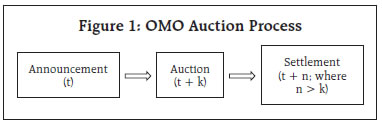 OMO auctions conducted by the central bank not only impact the quantum of liquidity in the economy but also government bond yields and other financial market instruments in terms of trading volume and volatility transmission. Based on Japanese tick-by-tick data, an empirical assessment of the immediate effects of notification of OMOs by the BoJ on trading volume and price volatility for the 10-year benchmark JGBs reveals that (i) outright OMOs increase the spikes in trading volume and price volatility in contrast to temporary OMOs (repurchase agreements); and (ii) unexpected changes in purchase amounts and notification times of OMOs increase the spikes (Inoue, 1999). In the context of the US, however, little systematic difference in market impact between OMO purchase and sale operations is found suggesting that the markets are potentially confused about the purpose of OMOs (Harvey and Huang, 2002). As the announcement effect of OMOs on G-sec yields has been examined earlier (RBI, 2021), the present exercise looks at the various domestic and global factors having an impact on the 10-year G-sec yields, based on daily data for the period January 2012 to March 2021. During this phase, 100 OMO auctions were conducted – 86 purchases and 14 sales. Therefore, the difference in closing yield of the previous trading day and the OMO auction day, controlled for other factors, captures the auction effect. Results from paired t-tests15 suggest negative and statistically significant softening in yields/rates, on an average, of (i) 2 basis points (bps) on announcement days: and (ii) 1 bp on auction days (Table 8). Similar tests for OMO sales announcements and auctions, however, suggest that the difference in yields is not statistically significant, hence the empirical exercise is confined to OMO purchases. The various domestic and global factors that are controlled for assessing the impact on 10-year G-sec yields are (i) changes in the policy repo rate (ΔPR); (ii) the size of the government market borrowing programme proxied by the market borrowing to G-sec market turnover ratio (GBR_T); (iii) the liquidity impact on yields (LIQUID) represented by the net LAF position as a proportion of NDTL of the banking system; (iv) volatility expectations in the Indian market as a proxy for India-specific uncertainty (INDVIX); (v) the 10-year US government bond yield (USYIELD) representing global factors; (v) positive domestic inflation surprises (AINFL_S) – consumer price index (CPI) inflation print being higher than the median estimate of professional forecasters – which have an adverse impact on long term bonds and the term premia; (vi) the lagged impact of changes in yields [GSEC (–1 to –2)] to reflect persistence16; (vii) the announced and auction amount as proportions of ₹10,000 crore (on an average, the usual auction size) on announcement dates (ANN) and auction dates (AUCT); and (viii) dummy variables for demonetisation period (DEM), taper tantrum (TT), pandemic (PAND) and quarter-end phenomenon (QDD) when banks reduce their lending exposure in the unsecured call market. | Table 8: Closing and Opening Rates – Paired t-test | | Variables | Window | Mean | t-stat. | p-value | | Announcement impact | | 10-year G-sec | Open (+1) - Close (0) | -0.02 | -2.22 | 0.01 | | Auction impact | | 10-year G-sec | Close (0) - Open (0) | -0.01 | -1.85 | 0.03 | Note: Open (0)/Close (0): Announcement/Auction day opening/closing.
Open (+1): Next day opening. | High frequency (daily) data of G-sec yields exhibit volatility clustering17, therefore, the generalised autoregressive conditional heteroscedasticity (GARCH) (1,1) framework (Bollerslev, 1986) is used with the mean and variance equation having the following specifications based on the variables mentioned above: 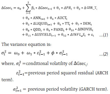 The diagnostics of the estimated model suggest that the volatility process is stable, and all coefficients are strongly significant with the expected sign; therefore, the model can be used for interpreting the estimated coefficients (Table 9). Change in the policy repo rate is found to have a direct impact on yields – an increase in the repo rate by 100 bps raises 10-year G-sec yield by 6 bps. As expected, higher market borrowing raises yields while increased liquidity has a sobering impact. While greater uncertainty and positive CPI inflation surprises raise yields, global disturbances like increasing US yields have a much stronger hardening impact suggesting the spillover effects of global factors on domestic financial markets. Controlling for the announcement effect, the impact of auction of about ₹10,000 crore is muted on yields. Finally, while yields hardened during the taper tantrum and during the quarter-ends, they softened significantly during the demonetisation and the pandemic period due to the ensuing liquidity glut. Overall, the findings suggest that 10-year yields are strongly influenced by global factors; in contrast, domestic factors have a more pronounced effect at the short-end as seen in the recent policy tightening phase. The above exercise is based on OMO auctions and not its variants such as OTs and G-SAP as separate analysis on those have been discussed earlier (RBI, 2021; RBI, 2022). | Table 9: Key Determinants of 10-year G-sec Yields | | Variable | Coefficients | | Constant | -0.001 | | ΣΔGSEC (–1 to –2) | -0.089*** | | ΔPR | 0.059*** | | GBR_T | 0.011*** | | ANN(-1) | -0.006*** | | AUCT | -0.009*** | | ΣOMO (Ann + Auc) | -0.015*** | | ΔLIQUID(-1) | -0.010*** | | TT | 0.084*** | | DEM | -0.016*** | | QDD | 0.022*** | | PAND | -0.011*** | | ΔINDVIX | 0.002*** | | ΔUSYIELD (-1) | 0.110*** | | ΔINFL_S | 0.010*** | | Variance Equation | | RESID(-1)^2 | 0.148*** | | GARCH(-1) | 0.598*** | | Diagnostics | | ARCH–LM test (p-value) | 0.1657 | Note: *, **, *** denote significance at 10, 5 and 1 per cent level, respectively.
Source: RBI staff estimates. | V. Conclusion The efficacy of OMOs in a market-based policy framework is well established in the literature as also in cross-country experiences on the operating procedure of monetary policy. It has gained importance in the Reserve Bank’s repertoire of liquidity management tools, particularly after the adoption of FIT. By reducing the policy lags, OMOs provide the wherewithal to the central bank in adopting a more nimble-footed approach while proactively managing liquidity conditions in consonance with the prevailing monetary policy stance. Besides altering liquidity conditions, OMOs also help in calibrating market expectations in sync with the monetary policy stance. The empirical exercise carried out in this article suggests that long-term (10 year) G-sec yields are significantly affected by global factors such as US financial market developments – much more than domestic factors like inflation surprises. In the present phase of policy tightening, the relatively synchronous movement of US long-term yields and domestic yields of similar maturities underscores this phenomenon. References: Arora, R, S Gungor, J Nesrallah, G O Leblanc and J Witmer (2021): “The Impact of the Bank of Canada’s Government Bond Purchase Program,” Bank of Canada, Staff Analytical Note 2021–23. Axilrod, S H (1997): “Introducing Open Market Operations, Reforms in Markets, and Policy Instruments” in T J T Balino and L M Zamalloa (eds), Instruments of Monetary Management – Issues and Country Experiences, International Monetary Fund, Washington DC. Bank for International Settlements (2019): “Unconventional Monetary Policy Tools: A Cross-country Analysis,” Bank for International Settlements, CGFS Papers No 63, October. Bernanke, B S (2020): “The New Tools of Monetary Policy,” American Economic Association Presidential Address, January 4. Bollerslev, T. (1986): “Generalized autoregressive conditional heteroskedasticity,” Journal of Econometrics 31, no. 3: 307–27. Das, S. (2020): “Seven Ages of India’s Monetary Policy”, Speech delivered at St. Stephen’s College, University of Delhi, January 24 Harvey, C.R., and R.D. Huang (2002): “The Impact of the Federal Reserve’s Open Market Operations”, Journal of Financial Markets 5, pp 223-257. Inoue, H. :(1999). “The Effects of Open Market Operations on the Price Discovery Process in the Japanese Government Securities Market: An Empirical Study,” CGFS Papers chapters, in: Bank for International Settlements (ed.), Market Liquidity: Research Findings and Selected Policy Implications, Volume 11, pages 1-21, Bank for International Settlements. Kuroda, H. (2016): The Practice and Theory of Unconventional Monetary Policy, in J. E. Stiglitz and M. Guzman (eds.), Contemporary Issues in Macroeconomics, Palgrave Macmillan Mandelbrot, B. (1963): ‘The Variation of Certain Speculative Prices’, Journal of Business, 36(4), pp 394-419. Mishkin, F S (1997): The Economics of Money, Banking and Financial Markets, Fifth edition, Addison-Wesley, Massachusetts, Boston. Patra, M. D., and I. Bhattacharyya (2022): Priming Monetary Policy For the Pandemic, Economic & Political Weekly, Money Banking & Finance, Vol LVII No 20, pp 41-48, May 14. Raj, J., Pattanaik, S., I. Bhattacharyya and Abhilasha (2018), “Forex Market Operations and Liquidity Management”, RBI Bulletin, August, pp 13-22. Rajan, R. G., (2016): Strengthening our Debt Markets, Annual Day Address to Foreign Exchange Dealers Association of India, Mumbai, August 26. Reserve Bank of India (2020): Governor’s Statement, October 9. Reserve Bank of India (2021): Monetary Policy Report, April 7. Reserve Bank of India (2022): Monetary Policy Report, April 8. Talwar, B A, K M Kushawaha and I Bhattacharyya (2021): “Unconventional Monetary Policy in Times of COVID-19,” RBI Bulletin, March, pp 41-56. Vlieghe, G. (2020): Monetary policy and the Bank of England’s balance sheet - Speech in an online webinar, April 23. Williams, J. C. (2020): A Time for Bold Action, Remarks at Economic Club of New York (delivered via videoconference), April 16.
ANNEX | Table 1: Open Market Operations – Select Country Practices (Contd.) | | Sr. No. | Name of the Central Bank | Repurchase OMOs | Forex Swaps | Central Bank Bills | Outright OMOs | | 1 | Reserve Bank of Australia | Every Wednesday morning, may do additional rounds on other business days and additional afternoon/evening rounds; these can be repo or outright | Short period swaps of usually not more than 3 months frequently conducted; Long-term swaps of up to 5 years also conducted | | Occasionally for government/semi-government securities of residual maturity >18 months (had conducted QE and YCC in response to the pandemic) | | 2 | Bank of Canada | Overnight and term repos | Yes | | Had conducted QE in response to the pandemic | | 3 | European Central Bank | Mostly one-week and 3-month tenor | May be conducted as fine-tuning operations | | Asset Purchase Programme launched in October 2014 and ended on July 1, 2022 (PEPP also conducted in response to the pandemic) | | 4 | Bank of Japan | Purchases for one year, sales for 6 months | Loans in foreign currency against pooled collateral for maximum duration of three months | The date of maturity of the bills must be within three months from the day following the sale date | Outright transactions in government securities, commercial paper, corporate bond, ETFs and J-REITs | | 5 | Bank of Korea | Mostly 7-day tenor | | Monetary Stabilization Bonds have relatively long maturities | Conducted limitedly in government/ government-guaranteed bonds | | 6 | Monetary Authority of Singapore | Intra-day, 28-day, 84-day | SGD-RMB swap facility of specified tenors for specified purposes | Monetary Authority of Singapore (MAS) bills are issued for tenor of 4/12 weeks; MAS floating rate notes for 6 month/1 year/2 year | | | 7 | Sveriges Riksbank | 7-day maturity | Yes | Riksbank certificates of 1-360 days maturity | Swedish government bonds were being purchased since 2015; in response to the pandemic SEK700 billion of government/covered/municipal/corporate bonds were purchased by December 2021 | | 8 | Swiss National Bank (SNB) | Repo transactions of tenor one day to several months; conducted daily | No liquidity providing foreign exchange swap outstanding since end-June 2012 | Issuance of SNB Bills for maximum tenor of one year (no outstanding since July 2012) | Purchase of SNB Bills in the secondary market | | 9 | Bank of England | Indexed Long Term Repo provides liquidity for 6 months; Contingent Term Repo Facility activated on need | Yes | | Asset purchases of gilts and corporate bonds completed and no-re-investment being done for maturing securities | | 10 | Federal Reserve System | Yes | Yes | | Various rounds of QE | | 11 | South African Reserve Bank | Yes | Yes | | Conducted during the pandemic | | 12 | Bank of Russia | Yes | Fine-tuning 1-2 day forex swap auctions | Bank of Russia bonds of 3/6/12 month terms | | | 13 | Reserve Bank of India | Yes | Yes | | Yes | | Source: Central banks’ websites (vetted mid-July 2022). |
| Table 2: Operation Twist (Special OMOs) | | (₹ crore) | | Date | Purchases | Sales | Net Purchases (+) / Sales (-) | | Announcement | Auction | Settlement | Amount notified | Amount accepted | Amount notified | Amount accepted | | 19-12-2019 | 23-12-2019 | 24-12-2019 | 10,000 | 10,000 | 10,000 | 6,825 | 3,175 | | 26-12-2019 | 30-12-2019 | 31-12-2019 | 10,000 | 10,000 | 10,000 | 8,501 | 1,499 | | 02-01-2020 | 06-01-2020 | 07-01-2020 | 10,000 | 10,000 | 10,000 | 10,000 | 0 | | 16-01-2020 | 23-01-2020 | 24-01-2020 | 10,000 | 10,000 | 10,000 | 2,950 | 7,050 | | 23-04-2020 | 27-04-2020 | 28-04-2020 | 10,000 | 10,000 | 10,000 | 10,000 | 0 | | 29-06-2020 | 02-07-2020 | 03-07-2020 | 10,000 | 10,000 | 10,000 | 10,000 | 0 | | 25-08-2020 | 27-08-2020 | 28-08-2020 | 10,000 | 10,000 | 10,000 | 10,000 | 0 | | 31-08-2020 | 03-09-2020 | 04-09-2020 | 10,000 | 7,132 | 10,000 | 10,000 | -2,868 | | 07-09-2020 | 10-09-2020 | 11-09-2020 | 10,000 | 10,000 | 10,000 | 9,900 | 100 | | 14-09-2020 | 17-09-2020 | 18-09-2020 | 10,000 | 10,000 | 10,000 | 10,000 | 0 | | 24-09-2020 | 01-10-2020 | 05-10-2020 | 10,000 | 10,000 | 10,000 | 10,000 | 0 | | 05-11-2020 | 12-11-2020 | 13-11-2020 | 10,000 | 10,000 | 10,000 | 10,000 | 0 | | 12-11-2020 | 19-11-2020 | 20-11-2020 | 10,000 | 10,000 | 10,000 | 10,000 | 0 | | 19-11-2020 | 26-11-2020 | 27-11-2020 | 10,000 | 10,000 | 10,000 | 10,000 | 0 | | 11-12-2020 | 17-12-2020 | 18-12-2020 | 10,000 | 10,000 | 10,000 | 10,000 | 0 | | 24-12-2020 | 30-12-2020 | 31-12-2020 | 10,000 | 10,000 | 10,000 | 10,000 | 0 | | 31-12-2020 | 07-01-2021 | 08-01-2021 | 10,000 | 10,000 | 10,000 | 10,000 | 0 | | 07-01-2021 | 14-01-2021 | 15-01-2021 | 10,000 | 10,000 | 10,000 | 10,000 | 0 | | 15-02-2021 | 25-02-2021 | 26-02-2021 | 10,000 | 10,000 | 10,000 | 10,000 | 0 | | 24-02-2021 | 04-03-2021 | 05-03-2021 | 15,000 | 15,000 | 15,000 | 15,000 | 0 | | 04-03-2021 | 10-03-2021 | 12-03-2021 | 20,000 | 20,000 | 15,000 | 10,895 | 9,105 | | 10-03-2021 | 18-03-2021 | 19-03-2021 | 10,000 | 10,000 | 10,000 | 4,750 | 5,250 | | 18-03-2021 | 25-03-2021 | 26-03-2021 | 10,000 | 10,000 | 10,000 | 10,000 | 0 | | 29-04-2021 | 06-05-2021 | 07-05-2021 | 10,000 | 10,000 | 10,000 | 10,000 | 0 | | 20-09-2021 | 23-09-2021 | 24-09-2021 | 15,000 | 15,000 | 15,000 | 15,000 | 0 | | 23-09-2021 | 30-09-2021 | 01-10-2021 | 15,000 | 15,000 | 15,000 | 15,000 | 0 | | Total | | | 2,85,000 | 2,82,132 | 2,80,000 | 2,58,821 | 23,311 | | Source: RBI. |
|