The article analyses volatility trend of currencies of select EMEs vis-à-vis US Dollar since 2007 covering major episodes of high-volatility such as the Global Financial Crisis, Eurozone Sovereign Debt Crisis, Taper Tantrum, Covid-19 outbreak, recent Russia-Ukraine conflict and Fed tightening of monetary policy. It also examines Indian Rupee’s volatility during these episodes and assesses the effectiveness of intervention by the Reserve Bank of India in curbing excessive volatility. The study finds that volatility expectations of the INR have come down over the study period. Further, the Reserve Bank has been able to achieve its intervention objectives over successive high-volatility episodes of global spillovers induced exchange market pressure. Introduction Currency volatility is a measure of the frequency and extent of changes in one country’s currency’s value vis-à-vis another country’s currency. It is measured by calculating the changes around the mean, expressed in terms of daily, weekly, monthly, or annual standard deviations. The larger the number, greater is the volatility over a period. In a world where sizable trades happen in currencies with market-determined exchange rates1, spikes in currency volatility are very common. While volatility of major currency (USD, Euro, Pound, Yen, Canadian Dollar, Australian Dollar, and Swiss Franc) pairs is usually low, that of Emerging Market Economy (EME) currencies (sometimes referred to as exotic currencies by traders) is relatively higher. Some of the important factors affecting volatility of a specific currency are interest rates, inflation, government debt, current account deficit, political stability, dependence on commodities as well as geo-political events. Further, overall liquidity of currency also matters, which is consistent with the fact that major currencies have lower volatility vis-à-vis so-called exotic currencies, with major currencies accounting for around 85 per cent of the turnover.2 Capital flows and associated exchange rate fluctuations affect macroeconomic and financial stability in EMEs through three main channels: (i) exchange rate pass-through to inflation; (ii) export competitiveness; and (iii) domestic financial conditions. The impact is more significant in EMEs than in advanced economies owing to their economic and financial structures (BIS, 2019). Thus, study of exchange rate volatility across EMEs is of paramount importance. With this backdrop, the article attempts to analyse volatility trend of currencies of select EMEs vis-à-vis the US Dollar since 2007. Section II covers volatility trends of the Indian Rupee, Indonesian Rupiah, Turkish Lira, Brazilian Real, South African Rand, South Korean Won, Philippines Peso and Thai Baht (first five were termed ‘Fragile Five’ currencies during the Taper Tantrum). The section also discusses realised volatility trends of select currencies. Section III further digs into volatility trend of the Indian Rupee, whereas Section IV discusses reasons for decline in volatility of EMEs in general and INR in particular. Section V concludes. II. Volatility trend of select EME currencies Trend of Implied Volatility To analyse the trend of volatility of select EME currencies, an equal-weighted implied volatility index of select EME currencies (one-month tenor) vis-à-vis US Dollar has been computed. As can be seen in the Chart 1, volatility has spiked quite a few times since 2007, most notably during the Global Financial Crisis (GFC) (2008-09), Eurozone Sovereign Debt Crisis (2010-11), Trade war (2018), onset of Covid-19 pandemic (2020), Russia-Ukraine conflict and Fed tightening (2022). Volatility measure for EME currencies was highest during the GFC with a peak value of around 40, whereas peak volatility levels are observed to trend lower in subsequent high volatility episodes mentioned above. 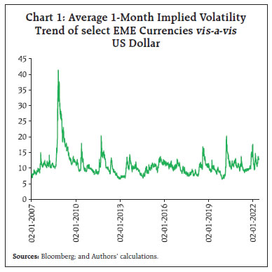 Another observation pertains to the tenor in each episode during which volatility has remained high i.e., above one standard deviation of computed index values . As can be seen in the Chart 2, it has also come down over the period from 203 trading days in GFC wherein values were more than one-sigma level of 14.71, to just one3 during the ongoing volatility phase (Russia-Ukraine conflict/ Fed tightening) (till end of May 2022). Moreover, average implied volatility during each of the episodes has also declined from around 23 during GFC to less than 15 during ongoing volatility phase. Generally, currency volatility is almost always associated with EME currencies or those of less-developed nations, though spikes in volatility are not totally uncommon4 in Advanced Economies’ (AE). Trend of Historical Volatility of select EM currencies Looking at the volatility of daily returns of select EM currencies on an individual basis vis-à-vis the US Dollar, it is observed that volatility of most currencies has fallen 2018 onwards relative to 2008-12 period (and in most cases relative to 2013-17 as well). Charts 3 and 4 plot the number of days the daily returns have exceeded one and two standard deviations. 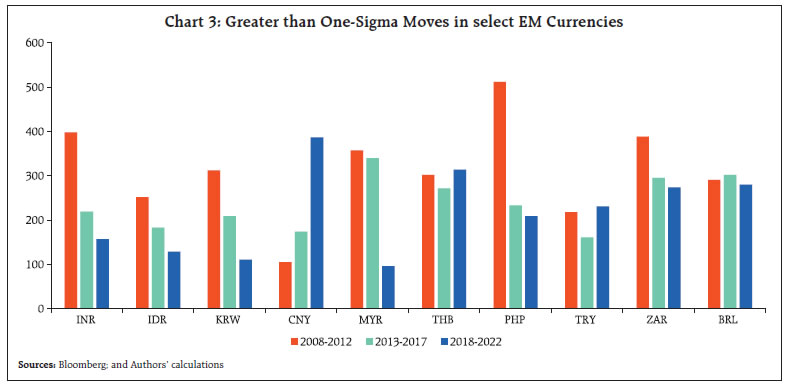 INR’s breach of 1-sigma level reduced from 398 days during 2008-12 to 157 days in the ongoing period. A similar trend is visible for the INR when we consider two-sigma moves. As regards the rise in CNY’s volatility, the same can be attributed to the depreciation of the currency during the trade-war era of 2018 and 2019 as well as around Covid outbreak in the first half of 2020. Further, introduction of a “countercyclical” component by China’s central bank in its model to calculate Yuan’s daily fix (central parity rate) in 2017 gave the central bank more control over the currency, making it harder for investors to predict the yuan’s value. The introduction of the counter-cyclical factor was seen to be increasing the weight of the discretionary part of the fixing by the bank and a step back from making the Yuan exchange rate more market driven (Chi Lo, 2017). Another study highlighted that the volatility of renminbi notably increased since the 2015 Yuan devaluation (Hong Kong Monetary Authority, 2021). Further, volatility has increased in case of Turkish Lira (TRY) and Thai Baht (THB) also, though to a lesser degree vis-à-vis CNY. 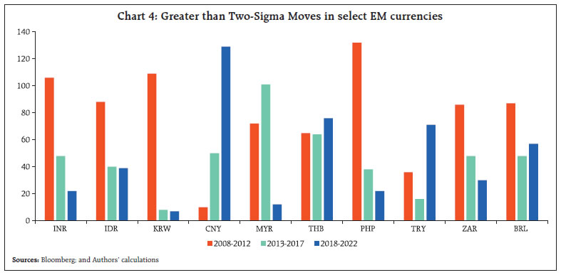 While currency volatility generally depends on economic fundamentals or country specific risks, factors such as delta hedging may also exacerbate it (Box 1) Box 1: Volatility in currencies due to Delta Hedging Traders provide liquidity by being willing to buy or sell options in return for compensation, but they get exposed to the potential large downside associated with short option positions. In this context, delta hedging allows traders to hedge the downside risk of short option positions (delta, one of the option greeks, measures change in the option position vis-à-vis change in the underlying asset’s price, while gamma is the rate of change in delta vis-à-vis change in the underlying’s price). However, delta-hedging is imperfect as delta changes with change in underlying asset’s price, thus requiring continuous rebalancing of the hedge. For options which are deep in-the-money or out-of-the-money or far from expiry, delta is generally stable (gamma is low), and there is lesser need to rebalance the hedge. However, for at-the-money options and/ or options approaching expiry, delta may fluctuate quickly, resulting in high gamma, making hedge rebalancing very difficult. (Iqbal, 2018). Traders monitor trend of the implied volatility of the currencies vis-à-vis historical volatility, while taking position in options. If the implied volatility for a currency pair (say USD-INR with USD being the base currency) is above historical standards, which results in the ratio of implied to historical volatility to be above 1, it may result in a view that volatility is over-priced. Thus, traders look to build short vega (vega is the rate of change in an option position vis-à-vis change in volatility of the underlying) position by selling options (for instance short straddle) which also results in short gamma position. If the traders’ expectations of low volatility are correct and market is confined within a specific range during the duration of the options contract, the strategy of selling options is profitable as the premium can simply be earned. However, if the currency breaks outside the expected range, the strategy exposes traders to unlimited risks. The more the currency moves, the more is the loss. For instance, if USD-INR level moves sharply upwards (i.e., INR depreciates), traders with a short call position will be forced to buy greater amounts of USD to hedge the exposure, whereas if the level moves sharply downwards (i.e., INR appreciates), traders with short put position have to short greater amounts of USD to limit losses. The ripple effect of such actions is that options players are the ones that assist the directional profile of a market (Evan, 2019). This is also the reason why a currency’s volatility increases during the expiry of options that have a large open interest. The spot market volatility increases if the hedge ratio of the trader, who has net short options (and therefore has a negative gamma exposure) is larger than the hedge ratio of the trader who has net long options. Further, typical option market makers (OMMs), e.g., large banks, dynamically hedge their positions, while option market takers (OMTs), e.g., investors, do not hedge their positions dynamically. This results in an asymmetric net delta hedge demand, which leads to an increase in the spot market volatility (if the OMM is short options or negative gamma) and vice-versa (Anderegg et. al., 2022). Some of the recent observations corroborate the findings of the above study. JPY’s depreciation vis-à-vis USD in April 2022 (it touched a 20-year low) intensified due to negative gamma positions (short call), while its 1-month implied volatility rose to highest level since 2017 (barring Covid-19 outbreak). Similarly, Yuan faced increased depreciation pressure due to covering of losses by traders holding short gamma position along with other factors, and its 1-month risk reversals rose to highest levels since March. 2020 on April 20, 2022. | III. Volatility Trend of the Indian Rupee The section analyses the general trend of INR volatility using various volatility measures and finds that the Reserve Bank has been able to achieve its objective of keeping INR’s exchange rate volatility low, which is reflected in trends of realised volatility, volatility cone and intraday range. Further, the currency’s volatility expectations have also come down over the study period as corroborated by trends in implied volatility, risk reversal and butterflies, etc. i. Implied volatility vis-à-vis historical volatility The historical volatility of the USDINR has remained below implied volatility most of the time (Chart 5). Further, if we look at the trend of implied volatility, we can see that it has reduced over the years. Therefore, notwithstanding occasional spikes, the hedging costs-as reflected by USDINR option premiums-has shown a downward trend which also points towards improvement in macro-economic and external sector fundamentals of India over the period as well as the confidence exhibited by the investors.
Not only has the spread remained in positive territory most of the time, it has also compressed over the last 15 years implying that the volatility predicted using option prices became more accurate over the years. Importantly, it also highlights that domestic forex market has deepened and has become more liquid over the period, allowing for proper pricing of instruments (Chart 6). ii. Volatility Cone Another way to view and compare spikes in volatility is volatility cone, which can be plotted using daily implied volatility values observed since 2007 across tenors. Highest realised volatility of INR during specific episodes can be compared vis-à-vis implied volatility’s historical highs, lows, median, etc., to gauge the extremity of movement in INR. Though the INR’s realised volatility was the highest during the Taper Tantrum, it is still below the highest implied volatility values observed during the study period across tenors. Importantly, during the ongoing crisis, highest one-month realised value is near the median implied volatility value (Chart 7). iii. High-Low spread Average high-low spread (in Rupee) has moved lower vis-a-vis the turbulent period of the taper tantrum, whereas the average of spreads as per cent of daily spot closing prices has also come down from about 0.80 in 2013 to around 0.40 levels in 2014 and is currently around 0.30 (Chart 8) iv. Risk Reversal The movement of the 25-delta risk reversal4 of the USDINR pair highlights that out-of-the-money call options have almost always been more expensive than the corresponding put options, implying expectations of depreciation of INR5 dominating expectations of appreciation (Chart 9). The market has always tilted towards depreciation of the Rupee, which, given the positive interest rate differential between India and the US, is expected. Although spikes have been observed during crisis events, similar to downward trend in implied volatility and IV-HV spread, the height of the spikes in RR, over the study period has declined, reflecting stronger economic fundamentals of India as well as effectiveness of RBI’s steps in controlling INR volatility.
v. Butterflies The trend of one-month butterfly6 for USDINR shows a distinct change in movement after 2015. Earlier, there were greater expectations of outsized movements with breaches above 0.6 not uncommon; however, post-2015, the measure has compressed, trending below 0.6 level most of the time (Chart 10). Further, the INR’s butterfly measure used to be much above CNY earlier, but it has now been trading near CNY’s levels, implying market expectations of outsized movements for INR have reduced considerably and are almost equal to that of CNY. This observation highlights the importance of India’s improved external metrics over years. vi. Term Structure of Volatility The trend of term structure of volatility (based on daily average) from 2009 to 2022 (till end-May 2022) shows that while daily average implied volatility was elevated with value exceeding 8 per cent for almost all tenors between 2009 to 2013, the curve fully submerged below the 8 per cent level in 2015 (Chart 11). Further, the curve never breached the 7 per cent level afterwards, implying that volatility expectations of INR have reduced in all tenors on a durable basis. vii. Volatility term spread The steepness of the term structure measured as the spread between implied volatility of 1-week /1-month tenors vis-à-vis 1-year tenor, has fallen over the years (except 2021), after having peaked in 2014, implying benign expectations of volatility across tenors (Chart 12). IV. EME Currency Volatility Post GFC, AE central banks flooded markets with liquidity whenever economic conditions became tough, dampening swings in asset prices generally, which involved large expansion of their balance-sheets (Chart 13). Further, as AE central banks largely moved in lockstep, the gaps between yields — key drivers of moves in exchange rates — also remained compressed. One of the important reasons of lower EME currency volatility over time is the accumulation of foreign exchange reserves by EME central banks. The trend has been evident post GFC, when liquidity infusion by AE central banks led to near/ sub-zero rates and yield hungry investors poured money into EMEs (Charts 14 and 15). 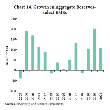 EME central banks accumulated reserves for a wide variety of reasons. A typical explanation highlights the precautionary role of holding reserves, though reserves were also accumulated as a by-product of other factors, including the pursuit of price and financial stability, and even export competitiveness (BIS, 2019). EMEs have experienced frequent crises since the 1980s: Latin America in the 1980s, Mexico in 1995, East Asia in 1997, Russia in 1998, Turkey in 1994 and 2001, Brazil in 1999, and Argentina in 2002 and 2018. One salient characteristic of these crises has been sudden stops in capital flows, which disrupted the financial system. Also given the absence of a fully adequate global safety net, EMEs have accumulated reserves in part as a form of self-insurance. Further, given the underlying uncertainty, judging reserve adequacy has remained very challenging, in turn, encouraging further prudence. The experience during and since the GFC indicates that reserves help EMEs navigate stormy waters. For example, during the GFC, the EMEs that held relatively more reserves experienced smaller currency depreciations, which was also the case during the taper tantrum in 2013. 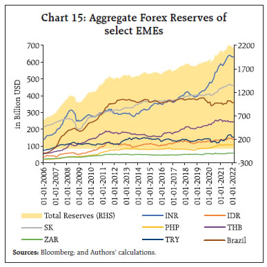
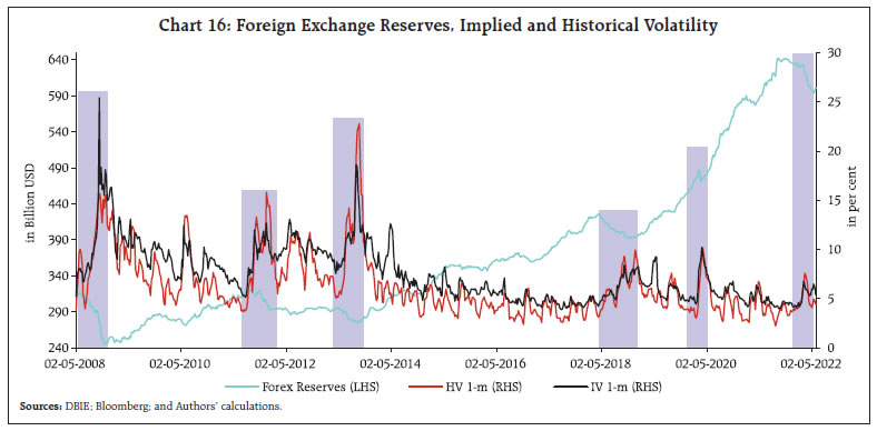 Decline in INR volatility Chart 16 depicts trend of domestic foreign exchange reserves along with the trends of 1-month implied and realised volatility of INR, with blue boxes highlighting trend of forex reserves and volatility during major crisis episodes. The declines in forex reserves are mainly on account of steps taken by the Reserve Bank during these episodes to contain excessive volatility. There has generally been a positive change in realised volatility (red portion above horizontal axis) along with a negative change in forex reserves (blue portion below horizontal axis) during each of the high volatility episodes, which has been followed by a negative change in realised volatility on a relatively durable basis (red portion below horizontal axis) (Chart 17). Moreover, the length and width of the blue portion below the horizontal axis has reduced generally over the study period, implying progressively lesser drawdown in forex reserves for containing volatility. For the period 2020 onwards (till the beginning of current high volatility phase), there has been a large accumulation of forex reserves by the Reserve Bank (the blue portion above the horizontal line). During large parts of the period between 2017-2021, the INR faced significant appreciation pressure on account of large-scale Foreign Portfolio Investors (FPI) and Foreign Direct Investments (FDI) inflows (barring downward pressure during 2018 and around Covid outbreak in 2020). Despite this, the realised volatility during this period has been low, as RBI absorbed a significant quantity of inflows in line with its objective of keeping the INR’s volatility low. 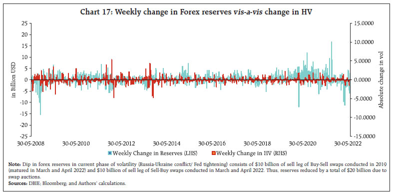 The drawdown in forex reserves was around $70 billion during the GFC which came down to $17 billion during Covid-19 outbreak (Chart 18). In the current Russia-Ukraine crisis and Fed tightening episode, while the drawdown in reserves stands at $56 billion (as on July 29, 2022), the net drawdown is much less when the depletion in reserves due to sell legs of swap auctions ($20 billion) and valuation losses is considered. Further, the size of the dip in forex reserves as a per cent to total forex reserves has come down from around 22 per cent during the GFC to six per cent during the Russia-Ukraine conflict and Fed tightening episode. This implies that due to a general reduction in volatility expectations of the INR over the study period and also because of accumulation and timely usage of foreign exchange reserves, the Reserve Bank has been able to achieve its intervention objectives with progressively lesser percentage drawdown in reserves. V. Conclusion The article analyses volatility trends of select EME currencies vis-à-vis the US Dollar since 2007. It also examines spikes in INR’s volatility during various episodes of global spillovers induced exchange market pressures and the effectiveness of the intervention by the Reserve Bank. The study finds that volatility expectations of the INR have come down over the time period. Further, the Reserve Bank has been able to achieve its intervention objectives with progressively lesser percentage drawdown in foreign exchange reserves. References: Anderegg, Benjamin, Ulmann, Florian and Sornette Didier (2022). The impact of option hedging on the spot market volatility. Journal of International Money and Finance 124, 102627. Arslan, Yavuz and Carlos Cantú (2019). The size of foreign exchange reserves. BIS Papers no. 104. Cai, Jun, Cheung, Yan-Leung, Lee, Raymond S.K. and Michael Melvin (2001). ‘Once-in-a-generation’ yen volatility in 1998: fundamentals, intervention, and order flow. Journal of International Money and Finance. Egea, Ivan Delgado (2019). What is Gamma Scalping and why it matters to trade forex markets. Accessed from https://www.nasdaq.com/articles/what-gamma-scalping-why-it-matters-trade-forex-markets-2019-01-04#:~:text=In%20a%20nutshell%2C%20gamma%20scalping,of%20a%20long%20gamma%20portfolio Bonanca, Jason J. (March 1999). Treasury and Federal Reserve Foreign Exchange Operations. Federal Reserve Bulletin. How Has the Value of the Pound Changed Since Brexit?. Accessed from https://www.ig.com/en/financial-events/brexit/value-of-the-pound-since-brexit Iqbal, Adam S. (2018). Volatility Practical Options Theory. Wiley. Lo, Chi (2017). PBoC introduces a ‘counter-cyclical’ factor in fixing of the renminbi. Accessed from https://investors-corner.bnpparibas-am.com/investing/pboc-introduces-a-counter-cyclical-factor-in-fixing-of-the-renminbi/
|