The article presents weekly activity indices to track the latest developments in the Indian economy with the least possible lag. Two different weekly indices have been developed using daily/weekly indicators – (i) a 7-indicator weekly activity index (WAI) using the dynamic factor model reflecting changes in economic activity on a year-on-year basis; (ii) a 15-indicator weekly diffusion index (WDI) reflecting directional movement on a sequential basis which compliments the model-based WAI. The WAI tracked the ebbs and flows in economic activity during the pandemic years followed by the more recent disruptions caused by the Russia-Ukraine war since February 2022. I. Introduction Outbreak of the COVID-19 pandemic called for prompt policy actions to safeguard livelihoods and make timely assessment of the economy to help in speedy recovery. With faster innovation and realignment of production processes due to the pandemic, the extant economic indicators fell short of keeping pace with rapid changes in the economy. This called for supplementing them with additional data, preferably with lower time lag. For the central banks, timely information on economic activity is crucial, particularly for exercising precise judgement in the monetary policy decisions. During each round of the monetary policy of the Reserve Bank of India (RBI), available information set for decision-making is found to be highly asynchronous. In terms of the data for the bimonthly policy, gross domestic product (GDP) is available quarterly and the conventional high frequency indicators (HFIs) at best on monthly basis with a lag of one or two-months (Table 1). During the August and February rounds of the policy, the information gap is especially large as the latest available official GDP data would lag by two quarters1. Moreover, the HFI set for the preceding quarter is not fully complete with no information available for the reference quarter. Leveraging the advancements in digitisation and automation, ministries, regulatory bodies and other private agencies are publishing additional economic data at a higher frequency. Such daily/weekly indicators available almost near real time, have the potential to bridge the information gap during the monetary policy rounds by supplying information till the week preceding the policy. | Table 1: Information Availability for Monetary Policy | | Round | Reference Quarter | Indicators Availability | Weekly Index
(complete up to) | | GDP | Monthly HFIs | | Complete | Partial | Scant | | April (t) | Q1 (t) | Q3 (t-1) | January | February | March | March | | June (t) | Q1 (t) | Q4 (t-1) | - | April | May | May | | August (t) | Q2 (t) | Q4 (t-1) | April, May | June | July | July | | October (t) | Q3 (t) | Q1 (t) | July | August | September | September | | December (t) | Q3 (t) | Q2 (t) | - | October | November | November | | February (t) | Q4 (t) | Q2 (t) | October, November | December | January | January | Note: 1. t indicates the current fiscal year.
2. Authors’ compilation. | In view of the above, this article presents weekly activity indices to track the latest developments in the Indian economy with least possible lag. Two different weekly indices have been developed using daily/weekly indicators – (i) a 7-indicator weekly activity index (WAI) using the dynamic factor model reflecting changes in economic activity on a year-on-year basis; (ii) a 15-indicator weekly diffusion index (WDI) reflecting directional movement on a sequential basis which compliments the model-based WAI. WDI presents sequential movement in activity to present an aggregate picture on the direction of trend movement. These indices apart from providing the weekly trajectory for the selected set of economic variables, also act as a robust indicator of the quarterly GDP. The rest of the article is structured as follows – section II provides an overview of the existing weekly indices developed by other central banks and private organisations, followed by a description of the constituent indicators in section III. Section IV discusses the methodology used in the construction of weekly indices. Section V presents the trajectory of the indices and their relationship with crucial macroeconomic indicators, viz., GDP and the index of industrial production (IIP). Section VI concludes highlighting the utility, existing limitations and future scope. II. Weekly Tracking in Central Banks Central banks, think tanks and other independent researchers engaged themselves in the practice of creating indices to nowcast/forecast economic activity with the available HFIs even before the pandemic. However, the search for an appropriate index intensified in the wake of abrupt economic developments during the outbreak of the pandemic. In the US, the Federal Reserve Bank of New York developed a weekly economic index (WEI) comprising a set of 10 HFIs (Lewis et al., 2020). The WEI is updated every Thursday with data till the preceding week, while also incorporating revisions, if any, for the earlier weeks. NY Fed’s WEI primarily gives a weekly picture of the real economic activity based on the latest available dataset at a fixed vintage, which is also tested to nowcast quarterly GDP growth. An unconventional weekly economic activity index for Germany created by the Deutsche Bundesbank used high frequency variables to track the quarterly GDP (Eraslan and Gotz, 2020). It used mixed frequency dataset comprising of the readily available high frequency variables along with the monthly industrial output and latest GDP estimate. The 13-week growth rates of the high frequency indicators are computed and a common factor within the mixed-frequency dataset is calculated by using principal component analysis (PCA). The index is viewed as rolling 13-week growth rate and at the end of a given quarter, the values of the index can be interpreted (in approximate terms) as quarter-on-quarter rate of change. Based on the data from five largest economies of the eurozone viz. France, Germany, Italy, the Netherlands, and Spain (comprising of 83 per cent of the eurozone output), the ING weekly economic activity index (ING-WAI) has been constructed by the ING to track the economic activity of the eurozone. Using the open access data on google search, google mobility, emission, energy consumption and trucking mileage, and a methodology similar to that of NY Fed and Bundesbank, the index shows the economic activity in the past week in comparison to the average over the entire data series. OECD also engages in real time tracking of economic activity of 46 countries (including India) through a series of three weekly trackers, one of which was discontinued at the end of 20212 while the other two continue to be updated. One of the two active trackers, provides estimates of weekly GDP relative to the same week in the previous year. The second one provides an estimate of weekly GDP relative to the same week two years before i.e., a 104-week difference. The trackers are computed by applying machine learning technique to a panel of google trends data and by aggregating together the information on search behaviour. The algorithm extracts and compiles information for various variables based on google search categories and collection of related keywords and groups them under separate heads such as consumption (e.g., “food and drink”, “autos & vehicles”, “households appliances”), labour markets (e.g. “unemployment”, “unemployment benefits”, “jobs”), housing (“real estate agency”, “mortgage”), business services (e.g., “venture capital”), bankruptcy (e.g., “bankruptcy”), industrial activity (e.g., “maritime transport”, “agricultural equipment”), trade (e.g., “exports”, “freight”) as well as economic sentiment (e.g., “recession”) and poverty (e.g., “food bank”). In India, both public and private stakeholders monitored the HFIs during the pandemic to track the course of economic activity under the emergency policy actions to contain the spread of infections. To name a few, the Narrow Recovery Index by Citi Bank, Business Activity Index by State Bank of India and Nomura India Business Redemption Index (NIBRI), became popularly discussed during the pandemic. As compared to February 2020 level (considered as 100), the NIBRI showed the activity status using Google’s daily community data on mobility around the workplace and retail and recreation spots, Apple Map’s index for driving mobility, weekly surveys on labour participation rate, and seasonally adjusted trends in weekly electricity demand. Owing to the country-wide lockdown induced restrictions, it was found that the activity dropped around 56 percentage points to a low of 44.4 by the end-April 2020. III. Data Description A total of 17 indicators dealing with different segments of the economy, have been considered which are broadly categorised into five buckets viz., soft, labour market, demand/sales, mobility, and payments (Table 2). | Table 2: High Frequency Indicators | | S. No. | Category | Indicators | Frequency | Source | | 1 | Soft | Google Trends | Daily | Google | | 2 | Consumer Sentiment Index | Weekly | CMIE | | 3 | Consumer Expectation Index | Weekly | | 4 | Current Economic Conditions Index | Weekly | | 5 | Labour | Unemployment Rate (%) | Weekly | | 6 | Labour Participation Rate (%) | Weekly | | 7 | Demand/Sales | Electricity Generation | Daily | Power System Operation Corporation Limited (POSOCO) | | 8 | Motor Vehicle Registration | Weekly | Vahan, Ministry of Road Transport and highways | | 9 | Railway Freight Loading | Daily | Ministry of Railways | | 10 | Air Cargo Traffic | Daily | Airport Authority of India (AAI) | | 11 | Mobility | Railway Passengers | Daily | Ministry of Railways | | 12 | Mobility (Retail, Grocery, Park, Transit & Workplace) | Daily | Google | | 13 | Aircraft Traffic | Daily | AAI | | 14 | Airport Footfall | Daily | AAI | | 15 | Payments | RTGS | Daily | RBI | | 16 | Retail Payments | Daily | | 17 | ATM and AePS Withdrawal | Daily | | Note: Retail Payments include National Electronic Funds Transfer (NEFT), Unified Payments Interface (UPI), Immediate Payment Service (IMPS), Bharat Bill Payment System (BBPS), Cheque Truncation System (CTS), Aadhaar Enabled Payment System (AePS) and National Automated Clearing House (NACH) payments. |
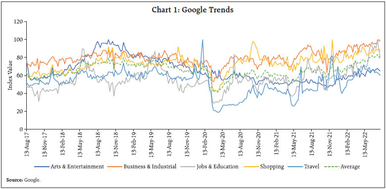 In the initial list of 17 indicators, long-time series were not available for a y-o-y comparison among a number of indicators as many were released for the first time during or after the pandemic outbreak. Accordingly, the indicators considered for the indices are a subset of the list presented in Table 2. The soft indicators viz., google trends data and the CMIE sentiment indices (consumer sentiments, current economic conditions, and consumer expectations) both of which are available since 2017 (Chart 1 and 2), showed a sharp dip during the first lockdown (March-April 2020). Sentiment indices particularly took a huge hit by around 60 index points. Recovery in the sentiments, which although on an upward trajectory, is still far below the pre-pandemic level. 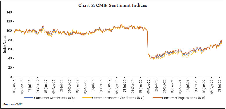
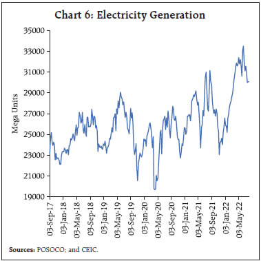
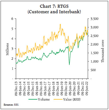
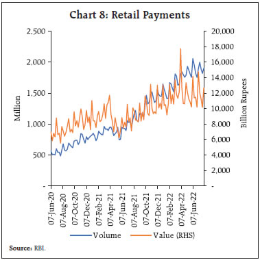
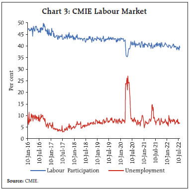 Labour market conditions are gauged through two indicators – unemployment rate and labour participation rate. Though no long-term trend is visible in the unemployment rate apart from the short-lived spikes during the first and the second waves, the labour participatipn has gradually declined in the recent past (Chart 3). For the model, the reciprocal of unemployment rate has been considered to control for the inverse relationship between unemployment and output. In the transport sector, passenger bookings and freight movement of the Indian railways also suffered sharp decline on account of the pandemic and the related uncertainty. Freight movement however registered a swift recovery (Chart 4). Vehicle registration and electricity generation are two important indicators of consumption demand. While the former tends to peak near the festive season (particularly during October-November) each year, electricity generation in addition to the upward trend over the past years, rises during every summer to meet the higher demand (Chart 5 and 6). 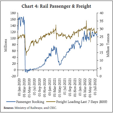 Payments data represent an unconventional source of tracing the underlying economic activity, given their crucial role in undertaking and settling transactions in a market economy (RBI, 2021). RTGS transaction (customer and interbank), which has been exhibiting an upward trend fecilitated by increasing digitisation, shows a seasonal peak at the end of every fiscal year (Chart 7). Retail payments (value and volume) data which RBI began publishing since June 2020 also exhibit similar upward trend. With majority of payments being made around the end of the month, a jump is visible in both value and volume of retail payments every month-end (Chart 8). Despite suffering a blow during the pandemic, both the data series have recovered well. Cash withdrawals from the ATMs recovered well after having suffered a dent in Q1:2021-22 (Chart 9). 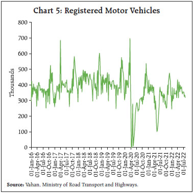
 Data on air cargo, aircraft movement and airport footfall are available on a daily basis only since June 2021 (Chart 10). Since the period is too short to be considered for the dynamic factor model (DFM), these data series have been used only in the diffusion index. With more data points collected in due course, air traffic data can be utilised in DFM for WAI as well.
An examination of the stationarity properties of the indicators shows that majority of them are stationary at first difference (Table 3). The correlation coefficient between the growth rates of the indicators aggregated at monthly and quarterly frequency with y-o-y real GDP and IIP growth have been examined prior to their inclusion in the model. Almost all the indicators exhibited strong correlation with target variables with expected signs. The magnitude of correlation is particularly strong in case of RTGS payments, electricity generation, google trends and vehicle registration (Table 4a and 4b). | Table 3: Stationarity of the Selected Indicators | | S. No. | Indicators | Diffusion Index | DFM-7 | Variable Transformation | | 1 | Google Trends | | √ | 1st Difference | | 2 | Consumer Sentiment Index (CSENT) | √ | √ | Level | | 3 | Unemployment Rate (Un Rate) | √ | √ | Level | | 4 | Labour Force Participation Rate (LFPR) | √ | √ | Level | | 5 | Electricity Generation (ElecGen) | √ | √ | 1st Difference | | 6 | Motor Vehicle Registration (MVReg) | √ | √ | 1st Difference | | 7 | Railway Freight Loading | √ | | 1st Difference | | 8 | Air Cargo Traffic | √ | | 1st Difference | | 9 | Railway Passengers | √ | | 1st Difference | | 10 | Mobility (Retail, Grocery, Park, Transit & Workplace) | | | Level | | 11 | Aircraft Traffic | √ | | 1st Difference | | 12 | Airport Footfall | √ | | 1st Difference | | 13 | RTGS | √ | √ | 1st Difference | | 14 | Retail Payments | √ | | 1st Difference | | 15 | ATM and AePS Withdrawal | √ | | 1st Difference | Note: 1. Google Mobility indicators are included only in the weekly activity index presented in level terms to exhibit the impact of different COVID-19 waves and subsequent resumptions in activities presented in Chart 12 in section 5.
2. First difference transformation for the variables is performed on year-over-year (y-o-y) basis for DFM and week-over-week (w-o-w) basis for Diffusion Index. |
| Table 4a: Correlation Matrix with Quarterly GDP growth | | | CSENT | LFPR | Un Rate | ElecGen | MVReg | RTGS | Google Trend | | CSENT | 1.00 | | | | | | | | LFPR | 0.82*** | 1.00 | | | | | | | Un Rate | 0.33 | 0.37 | 1.00 | | | | | | ElecGen | 0.46* | 0.61** | 0.49* | 1.00 | | | | | MVReg | 0.21 | 0.55** | -0.29 | 0.46* | 1.00 | | | | RTGS | 0.55** | 0.75* | 0.30 | 0.83*** | 0.64** | 1.00 | | | Google Trend | 0.70*** | 0.56** | 0.54** | 0.80*** | 0.24 | 0.60** | 1.00 | | GDP | 0.78*** | 0.90*** | 0.55** | 0.86*** | 0.48* | 0.86*** | 0.81*** | | Note: ***p < 0.01; **p<0.05; *p < 0.1. |
| Table 4b: Correlation Matrix with IIP Growth | | | CSENT | LFPR | Un Rate | ElecGen | MVReg | RTGS | Google Trend | | CSENT | 1.00 | | | | | | | | LFPR | 0.74*** | 1.00 | | | | | | | Un Rate | 0.33** | 0.40*** | 1.00 | | | | | | ElecGen | 0.40*** | 0.66*** | 0.51*** | 1.00 | | | | | MVReg | 0.13 | 0.53*** | -0.01 | 0.56*** | 1.00 | | | | RTGS | 0.51*** | 0.68*** | 0.28* | 0.72*** | 0.36** | 1.00 | | | Google Trend | 0.67*** | 0.57*** | 0.54*** | 0.76*** | 0.25* | 0.53*** | 1.00 | | IIP | 0.40*** | 0.79*** | 0.34** | 0.87*** | 0.83*** | 0.69*** | 0.59*** | | Note: ***p < 0.01; **p<0.05; *p < 0.1. | IV. Methodology The indices are expected to serve the two distinct purposes of (i) tracking developments in the real economy on year over year basis (WAI), and (ii) reflecting the sequential dynamics (WDI). For the above purpose, both model-based and simple aggregation approaches have been used, supported by a few sensitivity and robustness analysis. To monitor the economic recovery in level terms, relative to the pre-pandemic time, another version of WAI has also been developed. This is relevant during a period when there is heavy base effect and momentum serve as an appropriate yardstick to understand the pace of recovery, as it was the case during the pandemic. Activity as compared to the previous year may be improving, but it is equally crucial to know whether it is picking up with respect to immediately preceding period, or it has rebounded to the level existed before the shock, or is it able to sustain the recovery. DFM developed by Geweke (1977) and Sargent and Sims (1977), are the leading frameworks for the construction of a composite index from multiple time series. Factor model allows to use a rich dataset including large set of variables while dealing with the curse of dimensionality. The essence of DFM is to produce a small number of unobserved or latent series encapsulating the co-movements of the observed constituent indicators. Mathematically, the DFM posits the observed series as the sum of a vector of the common factors and that of idiosyncratic disturbances. In this study, DFM is used to forecast real GDP growth published at quarterly frequency based on the estimate of economic cycle represented by the monthly input variables, based on the approach specified in Giannone et al. (2008) and Banbura et al. (2011).  In the presence of a jagged edged data set, the dynamic relationship among the factors provides an edge over a static factor model by adding to the cross-sectional information and increasing the precision of the estimate of recent period with scarce information. The method used for estimating the unobserved factor Ft is the expectation-maximising (EM) algorithm under the state space framework, where the factor is estimated using the Kalman filter. DFM is useful for this purpose as a single model adopts to new data automatically as it becomes available to estimate the variable of interest3. An alternative approach to using HFIs for real time monitoring can be to forecast the specific economic variables and provide a model-based updates of the forecasts as and when new data comes. After estimating the WAI based on the constituent series, it is rescaled to track the quarterly real GDP growth. Apart from being the widely used macro-indicator, y-o-y GDP growth also aligns with the 52-weeks percentage change used for weekly seasonal adjustment. The scale and shift parameters are estimated using the following regression.
Weekly Diffusion Index The weekly sequential movement in activity has been presented in terms of a consolidated diffusion index using information from various indicators. The WDI, by construction, only present the direction of movement in activity and does not reflect magnitude. WDI has been constructed using a set of 15 indicators at weekly frequency starting from October 2020. The index is constructed following the methodology of the Conference Board4 showing the co-movement of multiple time series. It ranges between 0 and 100 and measures the proportion of the selected variables that contribute positively to the index. For example, an index value of 65 is interpreted as 65 per cent of the indicators registering week over week (w-o-w) acceleration, while index value of 50 implies w-o-w acceleration in 50 per cent of the total indicators. Construction starts with computing the w-o-w growth rates for each indicator. Indicators that grow by more than 0.5 per cent are given a value of 1, components that contract by more than 0.5 per cent are given a value of 0, and components with growth rates falling in between the range of 0.5 to (-) 0.5 per cent are given a value of 0.5. The values of the constituent series are aggregated, to obtain an index value between 0 to 100. V. Trajectory of the WAI Impact of the first COVID wave induced lockdown is evident from the deep downturn in the trajectory of the WAI (Chart 11). The milder impact of the second wave which is estimated to be around one-third in terms of loss of GDP was also corroborated by a decline in WAI levels (RBI, 2022). The third wave of COVID had no visible impact, except delaying the recovery, as exhibited by the WAI in the Month of February, March and April 2022. The value of 13-week MA of the WAI scaled to GDP (13-week MA) on the last week of a reference quarter encompasses the activity during that quarter and hence, is a rough nowcast of GDP growth for that quarter. Narrative of Indices Performance during Pandemic Unfolding of WAI trajectory can be seen in conjunction with the key events that took place during the two years since the outbreak of the pandemic. On March 11, 2020, the WHO declared COVID-19 as a global pandemic and on January 30, 2020 the first case of COVID-19 was reported in Kerala. Since then, India has experienced three waves of the pandemic, taking its total caseload to the second highest in the world. India imposed one of the most stringent restrictions in the world to curb the spread of infections during the first wave with the first phase of a nation-wide lockdown announced on March 24 continuing till the end of May 2020. Accordingly, the WAI for the week ending March 29, 2020 slipped to its lowest, contracting by 9.6 per cent on y-o-y basis, followed by contraction of 9.1 per cent and 8.9 per cent, respectively in April and May. The contraction in WAI was underpinned by broad-based decline in almost all the constituent indicators such as consumer sentiments, electricity generation, vehicle registration, various search categories of google trend, RTGS payment and skyrocketing unemployment rate. With gradual relaxations in restrictions, unlocking started since June 2020 over 6 phases - unlock 1.0 to unlock 6.0. Direct benefit transfers such as free ration per family members under the Pradhan Mantri Garib Kalyan Yojana followed by the Aatmanirbhar Bharat Abhiyan aimed at protecting jobs, providing financial support as well as regulatory relaxations, extensions, and guarantee schemes. As a result, V-shaped recovery was visible in some indicators such as RTGS transaction, electricity generation, unemployment, and labour force participation rates. Consumer sentiments, railway, air travel, vehicle registration, however improved at a slower pace. With the improvement in indicators, contraction in WAI also reduced steadily for 12 successive weeks since April last week till the second week of July 2020. With easing of contraction in each subsequent month in tandem with gradual unlocking, WAI turned positive in the second week of October 2020, after pandemic began to recede from its peak in September 2020. WAI aggregated over a quarter, which is available within a week after the end of a reference quarter and nearly two months before the official release of GDP data, tracked the quarterly GDP growth reasonably well in 2020-21. Hence, following the trend of quarterly GDP growth, WAI after two quarters of contraction, rebounded to positive territory in the third quarter and further strengthened in the fourth quarter of 2020-21. WAI’s approximate y-o-y changes were heavily influenced by base effects in 2021-22 emanating from the sharp contraction in 2020-21 and, therefore, obscured the subsequent impact of the COVID-19 waves in 2021-22. To address this issue, a weekly recovery index (WRI) is developed which is simply the WAI at levels, curated specifically for economic impact of different waves of the pandemic vis-à-vis., the pre-pandemic level (Chart 12). WRI surpassed its pre-pandemic level since the first week of December 2020. The launch of vaccination drive January 16, 2021 onwards, further bolstered momentum in economic activity which is reflected in sustained positive momentum in the index for fifteen successive weeks, till the second week of April 2021 when the second wave intensified. The economic impact of the second wave was moderate compared to the first wave. However, reinforcement of lockdowns by the central and the state governments thwarted economic recovery as the the WRI fell below the pre-pandemic level in May and June, 2021. The WRI rebounded in the first week of July with the plateauing of the second wave, removal of restrictive measures and government’s boost to accelerate vaccination drive and maintained steady momentum till September. Disruption caused by coal crisis, semi-conductor chip shortage across the globe started impinging on activity as was reflected in the downward trajectory in the recovery curve since late October and November 2021. Unlike the first two waves of COVID-19, the Omicron wave did not have any significant adverse economic impact as reflected by the WRI which remained above the pre-pandemic level in December and January 2022 and rebounded swiftly thereafter. Recent Trajectory: Since Russia-Ukraine War WAI recovered following a downturn during January caused by the Omicron wave. The WAI registered double-digit growth on average in the month of April and May 2022. However, the sharp uptick seen in these two months were partly due to the base effect emanating from the second wave. WAI moderated sharply in June and continued further on a downward trajectory in July 2022. The sequential movement evident from the weekly diffusion index (WDI) suggests continued sluggishness in momentum since March 2022. The 3-month MA of the WDI averaged at 61.1 for the months of February and March 2020, but moderated substantially thereafter, amidst the multiple headwinds arising from the ongoing Russia-Ukraine war (Chart 13). Out of 17 weeks from the first week of April to the week ending on July 24, the WDI remained below 50 on nine occasions. After touching 50 in May, 3-month MA of WDI deteriorated to 46.1 in June and further declined to 44.9 in July 2022. 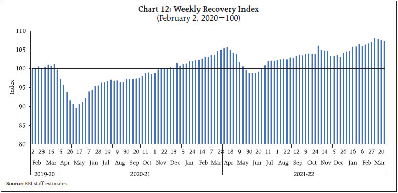
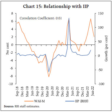
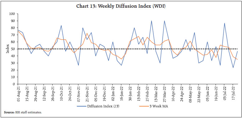 WDI presented since October 2020 displayed a sharp fall in momentum during the weeks of April 2021 when the second wave of COVID intensified. The index rebounded quickly in the subsequent months with more than half of the constituent indicators showing positive momentum. The index moved downwards in December 2021 and January 2022 primarily due to decline in employment rate and the third wave of pandemic. The Index rebounded sharply in February and remained resilient in March and April despite the headwinds in terms of spike in global commodity prices and supply disruptions as a fall out of the ongoing Russia-Ukraine war. Relationship with Macro-Aggregates The predictive relationship between the WAI and two primary macro indicators of output measures – real GDP and industrial production are also explored (Chart 14 and Chart 15). The quarterly average of WAI together with the y-o-y growth rate of real GDP exhibit strong co-movement over time. The correlation coefficient between two series also stood high at 0.79. The two months lag in the release of official GDP data makes it even crucial to look at the timely developments in the WAI. The quarterly aggregate of WAI scaled to GDP can provide a nowcast of GDP within a week since the end of the quarter. The monthly average of WAI tracks the y-o-y growth in IIP reasonably well with a correlation coefficient between the two series as 0.66. IIP for a particular month releases with a lag of forty-five days. Four-week average of the WAI which represents a month, on the other hand, become available within five days since the end of the month. Strong relationship with the lower frequency measures indicates that, despite the noise inherent in the raw high-frequency data, combining the indicators into a weekly index produces an informative and timely signal of real economic activity. 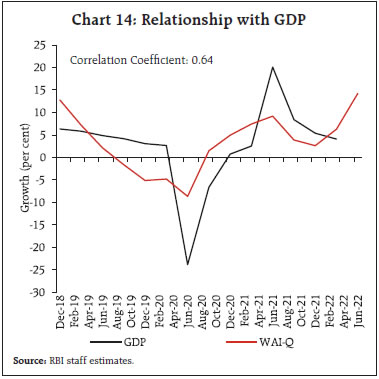 Forecasts being the natural application of the WAI, we further explore the predictive relationships between the WAI and lower-frequency real activity measures. We attempt to nowcast5 the target variable GDP by regressing the flow of information from the WAI, starting with the WAI for just the first month of the quarter and so on (Table 5a). 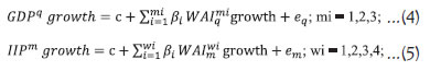
 Analogously, IIP is regressed starting with the WAI for the first week of the month and proceeded with additional information emanating from each subsequent week (Table 5b). The goal of these nowcasts is only to predict average variation in the target series over the frequency of the target variables which it performs well. For quarterly GDP, the WAI for all the three months is highly significant. However, the first month presents the strongest relationship with the highest value of adjusted R-square which decreases slightly over the next two months. In case of IIP, information from the first two weeks produced strongest relationship while the information from third and fourth weeks, despite remaining highly significant, did not improve the prediction further. Moreover, the Theil’s U statistic which is a relative accuracy measure that compares the forecasted results with the results of forecasting with minimal historical data, in case of both IIP and GDP stood less than one indicating that the WAI holds better predictive power over naïve forecast. | Table 5a: Monthly Information flow | | | WAI Month 1 | WAI Month 2 | WAI Month 3 | | Coefficient | 0.952*** | 1.034*** | 0.990*** | | Standard Error | 0.164 | 0.195 | 0.235 | | Adjusted R-square | 0.685964 | 0.64311 | 0.52790 | | F Statistics | 33.7652*** | 28.0304*** | 17.7730*** | | No. of Observations | 16 | 16 | 16 | | Theil’s U | 0.74136 | | | | Note: ***p < 0.01; **p<0.05; *p < 0.1. |
| Table 5b: Weekly Information flow | | | WAI Week 1 | WAI Week 2 | WAI Week 3 | WAI Week 4 | | Coefficient | 2.2845*** | 2.3015*** | 2.2548*** | 2.1884*** | | Standard Error | 0.3448 | 0.3425 | 0.3485 | 0.3576 | | Adjusted R-square | 0.4772 | 0.4844 | 0.4651 | 0.4368 | | F Statistics | 43.9043 | 45.1635 | 41.8636 | 37.4588 | | No. of Observations | 48 | 48 | 48 | 48 | | Theil’s U | 0.91980 | | | | | Note: ***p < 0.01; **p<0.05; *p < 0.1. | VI. Conclusion In a rapidly evolving economic situation, new sources of data to provide information about the current state of the economy have become a necessity for policymaking and economic analysis. In this respect, the WAI and WDI could serve as composite indicators of overall economic activity. This study finds that WAI tracks the ebbs and flows in economic activity during the pandemic years followed by the more recent disruptions caused by the Ukraine war since February 2022. Due to its timely availability, WAI holds the potential to bridge the information gap in the monthly high frequency indicators – a crucial input for monetary policy deliberations. The WAI tracks macroeconomic variables like monthly IIP and quarterly GDP reasonably well. In particular, the 4-week MA and the 13-week MA of the WAI provide nowcasts of IIP and GDP growth immediately after the end of the reference month or the quarter. To monitor the recovery relative to pre-pandemic time, WRI has also been developed showing the recovery in level terms. Unlike the first two waves of COVID-19, the Omicron wave did not have any significant adverse economic impact as the WRI moderated but remained above the pre-pandemic level in December and January 2022 and rebounded swiftly to an upward trajectory thereafter. WDI for a week presents momentum in economic activity by showcasing the overall direction where the economy is heading (upwards or downwards) in terms of a single index value. WDI is found to be useful in tracking the momentum in economic activity and suitably complements the model-based WAI. The weekly indices can supplement the more sophisticated nowcasting models of GDP. Presently, the set of daily and weekly high frequency indicators is limited but growing at a fast pace since the outbreak of the pandemic. Going forward, with the availability of sufficient data points, robust statistical and machine learning techniques can be used for enabling and strengthening real time tracking of real economic activity. References: Eraslan, S., and T. Gotz (2020), “An unconventional weekly economic activity index for Germany”, Technical Paper, Deutsche Bunesbank Eurosystem. Geweke, J. (1977), “The Dynamic Factor Analysis of Economic Time Series”, in Latent Variables in Socio-Economic Models, ed. by D.J. Aigner and A.S. Goldberger, Amsterdam: North-Holland. Giannone, D., L. Reichlin, and D. Small (2008), “Nowcasting: The Real-Time Informational Content of Macroeconomic Data”, Journal of Monetary Economics, 55, 665-676. Konings, Joana (2021), “Introducing the ING weekly economic activity index for the eurozone”, ING, Think Economic and Financial Analysis. Lewis, D.J., K. Mertens, and J.H. Stock (2020a), “Monitoring Real Activity in Real Time: The Weekly Economic Index”, Liberty Street Economics, March 30, 2020. https://libertystreeteconomics.newyorkfed.org/2020/03/monitoring-real-activity-in-real-time-the-weekly-economic-index/, accessed on May 22, 2022. Lewis, D. J., K. Mertens, and J. H. Stock (2020), “U.S. Economic Activity during the Early Weeks of the SARS-Cov-2 Outbreak”, Federal Reserve Bank of New York Staff Reports, no. 920, April. Lewis, D.J., K. Mertens, and J.H. Stock (2020b), “Tracking the COVID-19 Economy with the Weekly Economic Index (WEI)”, Liberty Street Economics, August 4, 2020. https://libertystreeteconomics.newyorkfed.org/2020/08/tracking-the-covid-19-economy-with-the-weekly-economic-index-wei.html, accessed on May 23, 2022. McCracken, M. (2020), “COVID-19: Forecasting with Slow and Fast Data”, On the Economy Blog, Federal Reserve Bank of St Louis. Reserve Bank of India (2021). Monetary Policy Report, October. Reserve Bank of India (2022). Report on Currency and Finance, October. Stock, J.H., and M.W. Watson (1989), “New Indexes of Coincident and Leading Economic Indicators”, NBER Macroeconomics Annual 1989, 351-393. Stock, J.H., and M.W. Watson (2002a), “Forecasting Using Principal Components from a Large Number of Predictors,” Journal of the American Statistical Association, 97:1167-1179. Stock, J.H., and M.W. Watson (2002b), “Macroeconomic Forecasting Using Diffusion Indices”, Journal of Business and Economic Statistics, 20:147-162. Woloszko, N. (2020), “Tracking activity in real time with Google Trends”, OECD Economics Department Working Papers No. 1634.
|