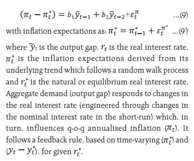
Revisiting the natural rate of interest in India with updated data, we obtain estimates in a range between 0.8 per cent and 1 per cent for Q3 of 2021-22, as against the range of 1.6–1.8 per cent estimated earlier for Q4:2014-15. Pandemic-induced factors have likely altered natural rate of interest which is sensitive to the choice of methodology and variables used, warranting careful interpretation within the assessment of the monetary policy stance.

Introduction

Since the 1990s, the natural rate of interest has transcended its Wicksellian origins and moved into centre-stage in the monetary policy apparatus of modern central banks that employ interest rates as their major policy instrument. The natural rate has emerged as a benchmark for assessing the policy stance. If the policy interest rate adjusted for inflation is higher than the natural interest rate, monetary policy is judged to be as anti-inflationary or contractionary. Analogously, if the real policy rate is lower than the natural rate, monetary policy is regarded as expansionary or accommodative. When the real policy rate is at or close to the natural rate, monetary policy is neutral, i.e., neither expansionary nor contractionary. This situation is expected to prevail when inflation is aligned to the target and output is at or close to its potential level.

The natural rate of interest is, however, unobserved in real life and has to be inferred from the data on its proximate determinants. It is determined by the efficiency of production, available amount of fixed and liquid capital, supply of labour and land (Wicksell, 1898); potential growth (Mendes, 2014; Garrison, 2006); demographics (Ikeda and Saito, 2014); fiscal policy and associated crowding-out effects (Engen and Hubbard, 2004); size of sovereign debt and default risk premium (Manasse et al., 2003); monetary policy shocks (Hanson and Stein 2015); financial cycles (Borio et al., 2019); globalisation and co-movement of real interest rates (Rogoff, 2006); and a host of heterogenous factors like fertility rate and life expectancy, inequality, relative price of capital goods, investment sentiment, capital flows and risk premium (Borio et al., 2017; IMF, 2022)¹. Consequently, the natural rate of interest, or r-star as it has come to be referred to in central banking parlance, becomes an empirical question (Wieland, 2018). Accordingly, accurate and statistically robust estimation of r-star and regular update of these estimates is a valid operational pursuit in the context of the conduct of monetary policy.

Estimates of the natural rate are notoriously imprecise, which weakens their utility as a reference guidepost for monetary policy. First, empirical estimation is inevitably model-driven and extremely methodology sensitive, with confidence intervals of imprecision. Model-specific differences and statistical uncertainties of estimates pose formidable obstacles to passing a judgement on the level of the natural rate of interest in real time (Brand et al., 2018). Second, these estimates also tend to be sensitive to the choice of time horizon – short-term, medium-term or long-term – and hence to the nature of shocks (i.e., whether they are temporary or structural and long-lived); the measure of inflation; and, the choice of underlying determinants. Third, it is important to be reminded by prescient voices in the literature that incorrect estimation of the natural rate could lead to significant welfare cost (Orphanides and Williams, 2002). Consequently, a central bank may generally talk about the level of interest rates that would broadly be neutral, instead of conveying any precise number (Chetwin and Wood, 2013).

In the post-pandemic world, identification of the level of this neutral interest rate has become even more challenging because several determinants of the natural rate have exhibited distinct shifts, with persisting uncertainty about whether and over what time frame they may normalise. The trajectory of potential growth, a key determinant of the natural rate, may rise due to large increase in public spending on infrastructure, digitisation, push to innovation from start-ups and new business opportunities, but it may also decline due to the scarring effects of the pandemic on education, labour market, globalisation, growing state influence in the economy and market concentration, and hence on productivity (Gromling, 2021; Tanaka et al., 2021). Pandemics typically depress investment demand, because of the overwhelming preference of households to save more/rebuild depleted wealth rather than consume, and as a result, the natural interest rate post-pandemic may decline by nearly 1.5 percentage points, reaching its lowest point after about 20 years, and then taking equal number of years to return to the pre-pandemic level (Jorda et al., 2020). While higher public spending and government debt could raise the r-star, a drop in desire to invest by the private sector and an increase in desire to save by the households may lower it, with the net impact likely to remain uncertain (Adolfsen et al., 2021). Two opposing forces – high public debt and expenditure on the one hand and the unusual swell in savings on the other – could influence the evolution of the natural rate post-COVID (Goy and End, 2020; Bismut and Ramajo, 2021). Extra caution, however, would be advisable while estimating the natural rate because the impact of the ongoing structural transformations ranging from climate change to the rise of shadow banking and fintech may be hard to approximate (IMF, 2022). Thus, for monetary policy assessment, what one can get is a broad range rather than a bright line drawn on the road: “It’s not something we can identify with any precision. So we estimate it within broad bands of uncertainty” (Powel, 2022)².

In India, net household financial savings surged to about 16 per cent of GDP in Q1:2020-21 during the first wave of the pandemic, from 8.0 pr cent of GDP during the financial year 2019-20, before moderating in the subsequent three quarters. During the second wave of the pandemic, it surged again to 14.8 per cent of GDP in Q1:2021-22 (RBI, 2022). On the other hand, general government debt increased to 89.4 per cent in 2020-21 (from 75.7 per cent in 2019-20) and is likely to remain sticky at around 84 per cent of GDP over the next five years (RBI, 2022). The potential growth of India is also assessed to have declined to marginally below 6 per cent post-COVID (RBI, 2022; Patra et al., 2021), though the steady state growth path is likely to normalise/rise to a range of 6.5 - 8.5 per cent in the medium-term as the beneficial impact of reforms in the pipeline as well as new reforms gain traction³. In the labour market, the labour force participation rate plummeted after the pandemic struck, which is yet to normalise (RBI, 2022). According to the recent National Family Health Survey (NFHA), India’s fertility rate has consistently declined over the last three decades to marginally below the replacement rate. Sharp changes in these underlying drivers of the natural rate call for a revisit of the estimates. This assumes relevance in the context of the recent observation that “It is time now (for the RBI) to withdraw crisis time accommodation in terms of moving towards the equilibrium or neutral real rates consistent with non-inflationary growth” (Goyal, 2022)⁴.

Set against this background, the main motivation of this article is to update estimates of r-star for India provided in Behera et al. (2015), while also exploring new estimates that incorporate the effects of financial cycles. Section II presents the theoretical framework used for estimation of the natural rate. Empirical results are set out in Section III. Concluding observations are given in Section IV.

2. Theoretical Framework for Estimation

The methodology used in this article follows the seminal work of Laubach and Williams (2003) (LW, henceforth) and its extended version (Juselius et al., 2016)⁵. In essence, the LW framework combines robust theoretical relationships embodied in Ramsey’s growth model and the standard New Keynesian or neo-Wicksellian policy dynamics with the Kalman filter estimation technique, in order to model unobservable/ unknown macro-dynamics. In the New Keynesian framework, the natural rate of interest is time-varying and could be influenced by shocks impacting both aggregate supply and aggregate demand.

If the time preference to consume today relative to tomorrow is high, r must exceed ρ to encourage saving today. The extent by which saving may increase will depend on the intertemporal elasticity of substitution. By rearranging (1):

The more general reformulation, as considered by LW, is presented below:

A modified version of equation (3), which considers a slow adjustment process in the movement of the natural rate, can be written as: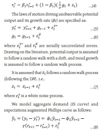

An important channel through which monetary policy could alter the trend real interest rate is the financial cycles (Borio et al. 2019). Incorporating financial cycles into a modified LW framework ensures that the equilibrium real interest rate is consistent not only with the requirement of actual output at close to potential and actual inflation close to its long-term trend but also with a state of financial equilibrium. Financial booms and busts can have permanent effects on output, and therefore, a measure of the natural rate that can also help limit financial disequilibrium in the system could also effectively help reduce output effects of financial booms and busts. The LW framework is augmented by incorporating the leverage gap as a proxy for the financial cycle, i.e., a measure of the leverage gap is introduced in the IS curve as a determinant of the output gap and a separate equation is added for the leverage gap (Juselius et al. 2016 and Borio et al. 2019).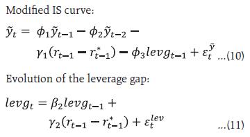

The leverage gap is estimated by first establishing a cointegrating relationship between credit to GDP ratio (cred) and real asset prices (rap), and then taking deviations from its steady state equilibrium relationship:

When the leverage gap is negative, that would indicate that asset prices are bullish, and through positive collateral valuation effects, the credit to GDP ratio could increase, leading to higher output. This inverse relationship between the leverage gap and the output gap in the modified IS curve is presented in eq. (10). The real interest rate gap (i.e., actual real interest rate minus the natural rate) matters for the leverage gap, as presented in eq. (11). If the actual real rate is above the natural rate, asset prices should decline to increase the leverage gap.⁶ The real interest rate is the difference between nominal policy rate (i_t) and inflation expectations (π_t^*), where i_t is based on a Taylor-type rule: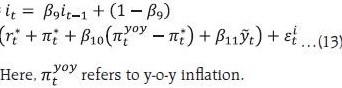

Quarterly data for various macroeconomic variables for the period 1999:Q4 to 2021:Q4 are used. GDP data are obtained from the website of the National Statistical Office with appropriate splicing (Bhoi and Behera, 2017). GDP data are adjusted for COVID-19 shocks (Patra et al., 2021). Data on consumer prices (CPI-combined), short-term nominal interest rates (91-day Treasury bill yields), bank credit and BSE Sensex (as a proxy for India’s equity prices) are taken from the Database on Indian Economy (https://dbie.rbi.org.in). The underlying real interest rate (r) used in the model is worked out by taking the difference between 3-month Treasury bill yields⁷ and the underlying trend inflation. The trend inflation, estimated endogenously within the model, is used as a proxy for inflation expectations. Real GDP, CPI, bank credit and equity prices are adjusted for seasonality using US Census X-13 ARIMA-SEATS⁸. The real equity price (rap) series is constructed by deflating seasonally adjusted equity prices with seasonally adjusted CPI inflation. The credit to GDP ratio variable is generated by dividing bank credit with nominal GDP.

In order to estimate the model with latent factors, the standard practice is to use maximum likelihood estimation (MLE) methods (Laubach and Williams 2003; Clark and Kozicki 2005; Behera et al. 2017; Holston et al. 2017). Here, the main challenge is fixing relevant priors on parameters, giving rise to the ‘pile-up problem’⁹, as the contributions from variations in some of the variables used in estimation to overall variability in the data are relatively small (Me´sonnier and Renne 2007; Laubach and Williams 2003; Stock and Watson 1998; Stock 1994). Consequently, maximum likelihood estimates tend to be biased, which can be mitigated by using the median unbiased estimator procedure, but it is based on a very precise implicit prior belief about the volatilities of latent factors and, therefore, highly restrictive (Lewis and Vazquez-Grande, 2018). To overcome these problems, we have used Bayesian methods with relatively loose priors on different parameters¹⁰. This not only provides a solution to the pile-up problem, but it also generates estimates which are more reliable (Primiceri 2005; Lewis and Vazquez-Grande 2018; Kim and Kim 2018).

Johansen maximum likelihood estimation results suggest the evidence of one cointegrating relationship, as the null hypothesis of ‘no cointegration’ is rejected at 5 per cent level of significance. The estimated leverage gap for India seems to capture credit booms and episodes of asset price bubbles and busts reasonably well (Chart 1). For the more recent period i.e., 2018-21, the leverage gap would suggest that asset (equity) prices are relatively bullish compared with the credit-GDP ratio in the economy, resulting in a negative leverage gap. If a “lean against the wind” policy is pursued, then asset prices could get better aligned with the credit to GDP ratio¹¹.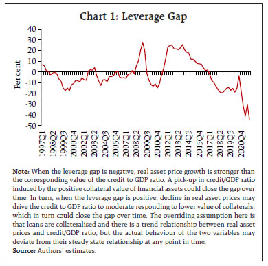

Employing a Bayesian approach as stated earlier, we have estimated the baseline LW version (eqs. 4 to 9’) and the modified LW version adjusted for financial cycle (replacing equation 8 with eq. 10 and adding eqs. 11 and 13). Given that the parameter set is large, we avoid specifying priors that are fully non-informative and consider a beta distribution for prior parameters for the coefficient value of all variables and a gamma distribution for shock variances. The assumptions on specifying the means and standard deviations of the priors are mostly motivated by existing estimates for India in the literature as well as estimates from HP filtered series of different variables wherever parameter estimates are not available in the literature. We calibrate the rate of time preferences (ρ) with a value equal to 0.99 in line with the literature. As we have estimated the model with non-stationary variables, we use diffuse Kalman filter along with Metropolis-Hastings algorithm to estimate the model. Each set of results is based on 180,000 posterior draws while considering an initial 50 per cent draws as burn-in. For computing each marginal likelihood value, we use 90,000 important sampling draws.

3. Empirical Results

The posterior estimates of the parameters in the model are found to be different from the priors, making them suitable for use to estimate the natural rate (Table 2). The posterior estimates indicate that the output gap is significantly influenced by the leverage gap (a la Rath et al., 2017 and Juselius et al., 2016). Some caveats, however, need to be recognised. First, the inclusion of the leverage gap in the IS curve equation increases persistence of the output gap, implying a weaker influence of monetary policy (or real interest rate gap) on demand conditions (or output gap). Second, the leverage gap also exhibits a high degree of persistence, indicative of long-run effects on the output gap. Third, we did not find a major role of monetary policy in influencing financial cycles in India as the coefficient of the real interest rate gap (γ₂) in the leverage gap equation is small.

Impulse responses from the estimated model suggest that a positive shock to the interest rate leads to an equivalent increase in the real interest rate gap, which lowers the output gap and inflation and also narrows the leverage gap. The magnitude of the impact on the leverage gap is relatively small though, and it also involves greater lags (Chart 2). This suggests that the use of macro-prudential measures instead of monetary policy may be the preferred policy option to stabilise the leverage gap.

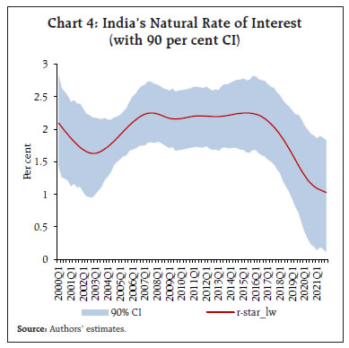
The results indicate that since 2014, growth in potential output has decelerated, and the output gap measures¹² show the presence of slack in the economy, which is in line with the findings of Patra et al. (2021) (Chart 3). Correspondingly, the natural rate is estimated to have declined to 1 per cent, with a higher confidence band (lower band at 0.15 per cent and the upper band at 1.9 per cent) to reflect the impact of post-COVID volatility in key determinants of the natural rate (Chart 4).

While LW based estimates using different measures of inflation (i.e., headline and core CPI) produce more or less similar time varying behaviour of the natural rate of interest, the estimates incorporating leverage dynamics produce different set of estimates (Chart 5). For Q3:2021-22, LW estimates are in the range of 0.8 per cent (when core CPI inflation is used as the deflator) to 1.0 per cent (when headline CPI inflation is used as the deflator), with a wide confidence band of around +/- 90 bps. Corresponding modified LW estimates are in the range of 2.0 per cent to 2.1 per cent with a confidence band of around +/- 60 bps.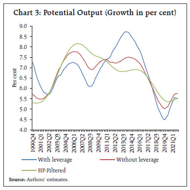

Available estimates of the natural rate of interest for India in the literature during the last decade offer useful insights. The trend level of the real policy rate in India derived from application of statistical filters declined by more than 200 basis points after the global financial crisis (Perrelli and Roache, 2014). Large downward shifts in estimated natural rates after the global financial crisis have been reported in the literature for both advanced and emerging economies. Natural rates in the Asian economies also declined after the global crisis, reflecting lower trend GDP growth at home and a lower global neutral rate. Three different methodologies – theoretical calibration; semi-structural modelling; and extended Taylor rule – suggested a decline in India’s natural rate after the global crisis to 2.6 per cent, 4.2 per cent and 1.1 per cent, respectively (IMF, 2015). Another study for the BRICS countries highlighted that in India the real interest rate has been systemically kept below the equilibrium value and must be raised (Klose 2018). A counter view is evident from the findings of Goyal et al., (2016), which highlighted that periods when the policy interest rate in India exceeded the natural rate were far more frequent, and as a result, monetary policy was largely contractionary. Thus, in the pre-pandemic period, different estimates were used to draw divergent inferences on the stance of monetary policy. Post-COVID, notwithstanding the higher uncertainty band around the estimated natural rate of India, it may be appropriate to infer that the natural rate might have moderated somewhat, as suggested by the decline in comparable estimates from a range of 1.6 -1.8 per cent¹³ in Q4:2014-15 to 0.8 -1.0 per cent in Q3:2021-22.

5. Conclusions

This article highlights why point estimates of the natural rate of interest may vary significantly over time, and more importantly, why the estimated values of the natural rate of interest may lie within a wide range at any point in time, depending upon the choice of methodology, model assumptions and the nature of the data. For India, our estimates of the natural rate for the post-pandemic period suggest a range of 0.8 per cent to 1.0 per cent for Q3 of 2021-22, which is lower by about 80 basis points than the earlier comparable estimate of 1.6-1.8 per cent for Q4:2014-15. This decline is consistent with the assessed moderation in growth of potential output during the corresponding period. Reflecting greater uncertainty surrounding the estimation of the natural rate post-Pandemic arising from more volatile paths of some of the key underlying drivers of the natural rate, the confidence band around the estimates has increased to +/- 90 basis points, as against +/- 50 bps for 2014-15.

An alternative model that takes into account both financial cycles and business cycles to generate the equilibrium real interest rate recognises the dynamic interactions between them, in the context of the debate on whether monetary policy must “lean against the wind” to avoid asset price bubbles. The alternative estimates of natural rate as per this approach turn out to be higher in the range of 2.0-2.1 per cent for Q3:2021-22, reflecting the post-pandemic negative leverage gap, i.e., the real asset prices being more bullish than prevailing credit market conditions, that may require higher interest rates than warranted to effectively lean against the wind to restore equilibrium. Impulse response analysis, however, shows that the magnitude of the impact of higher real interest rates on the leverage gap is relatively small and it also works with greater lags. Thus, even as financial cycles tend to influence the output gap, the sensitivity of leverage gap to changes in real interest rate is estimated to be modest, which could be interpreted as a case against using monetary policy to “lean against the wind”.

References

Adolfsen, J.F., Rasmussen, T.T.I., and Pedersen, J. (2020). “How does COVID-19 affect r*?”, Economic Memo, No. 14, December, Danmarks Nationalbank.

Behera, H. K., Pattanaik, S., and Kavediya, R. (2017), “Natural Interest Rate: Assessing the Stance of India’s Monetary Policy under Uncertainty”, Journal of Policy Modeling, 39(3), 482-498.

Behera, H. K., Pattanaik, S., and Kavediya, R. (2015). “Natural Interest Rate: Assessing the Stance of India’s Monetary Policy under Uncertainty”, RBI Working Paper WPS(DEPR)/05/2015

Bhoi, B. K., and Behera, H. K. (2017). “India’s Potential Output Revisited”, Journal of Quantitative Economics, 15(1), 101-120.

Bismut, C., and Ramajo, I. (2021). “ Nominal and Real Interest Rates in OECD Countries, Changes in Sight After Covid-19?”. International Economics and Economic Policy, 18(3), 493-516.

Borio, C., Disyatat, P. and Rungcharoenkitkul, P. (2019). “What Anchors for the Natural Rate of Interest?”, BIS Working Papers No 777, March.

Borio, C., Disyatat, P. Juselius, M. and Rungcharoenkitkul, P. (2017) “Why So Low for So Long? A Long-term View of Real Interest Rates”, BIS Working Papers No 685, December.

Brand, C., Bielecki, M., and Penalver, A. (2018). “The Natural Rate of Interest: Estimates, Drivers, and Challenges to Monetary Policy”, ECB Occasional Paper, No. 217.

Clark, T. E. and Kozicki, S. (2005), “Estimating Equilibrium Real Interest Rates in Real Time”, The North American Journal of Economics and Finance, 16(3), 395-413.

Chetwin W. and Wood, A. (2013). “Neutral Interest Rates in the Post-crisis Period”, URL: http://www.rbnz.govt.nz/research_and_publications/analytical_notes/2013/an2013_07.pdf.

Engen, E. M., and Hubbard, R. G. (2004). “Federal Government Debt and Interest Rates”, NBER Macroeconomics Annual, Cambridge, Massachusetts: National Bureau of Economic Research, 83-138.

Garrison, R.W. (2006). “Natural and Neutral Rates of Interest in Theory and Policy Formulation”, Quarterly Journal of Austrian Economics, 9(4): 57-68.

Goy, G. and End, J.W. (2020). “The Impact of the COVID-19 Crisis on the Equilibrium Interest Rate”, VoxEU, CEPR, April 20.

Goyal, A., and Arora, S. (2016). Estimating the Indian Natural Interest Rate: A Semi-structural Approach. Economic Modelling, 58, 141-153.

Grömling, M. (2021). COVID-19 and the Growth Potential. Intereconomics, 56(1), 45-49.

Hanson S.G. and Stein J.C. (2015). “Monetary Policy and Long-term Real Rates”, Journal of Financial Economics, 115: 429-448

Holston, K., Laubach, T. and Williams, J. C. (2017), “Measuring the Natural Rate of Interest: International Trends and Determinants”, Journal of International Economics, 108, S59-S75.

Ikeda, D. and Saito, M. (2014). “The Effects of Demographic Changes on the Real Interest Rate in Japan” Japan and the World Economy, November, 32: 37-48

International Monetary Fund (2015). Regional Economic Outlook: Asia and Pacific, April.

--- (2022). World Economic Outlook, Washington D.C., April.

Jordà, Ò., Singh, S. R., & Taylor, A. M. (2020). “The Long Economic Hangover of Pandemics”, Finance & Development, 57(2), 12-15.

Juselius, M., Borio, C., Disyatat, P. and Drehmann, M. (2016). “Monetary Policy, the Financial Cycle and Ultra-low Interest Rates”, BIS Working Papers, No. 569.

Juselius, M. and Drehmann, M. (2015), “Leverage Dynamics and the Real Burden of Debt”, BIS Working Papers, No. 501.

Kim, C. J., and Kim, J. (2018), “Trend- Cycle Decompositions of Real GDP Revisited: Classical and Bayesian Perspectives on an Unsolved Puzzle”. Available at SSRN: http://dx.doi.org/10.2139/ssrn.2883438

Klose, J. (2020). Equilibrium Real Interest Rates for the BRICS Countries. The Journal of Economic Asymmetries, 21, e00155.

Laubach T., Williams J.C. (2003). “Measuring the Natural Rate of Interest”, The Review of Economics and Statistics, 85(4): 1063-1070.

Lewis, K. F., and Vazquez-Grande, F. (2019). “Measuring the Natural Rate of Interest: A Note on Transitory Shocks”, Journal of Applied Econometrics, 34(3), 425-436.

Manasse, P., Roubini, N., Schimmelpfennig, A. (2003). “Predicting Sovereign Debt Crises”, IMF Working Paper, No. 03/221.

Mendes, R.R. (2014). “The Neutral Rate of Interest in Canada”, Bank of Canada Discussion Paper, September.

Me´sonnier J.S. and Renne J.P. (2007). “A Time-varying ‘‘Natural’’ Rate of Interest for the Euro area”, European Economic Review, 51: 1768–1784.

Orphanides, A. (2019) “Monetary Policy Strategy and its Communication”, Federal Reserve Bank of Kansas City 2019 Jackson Hole Economic Policy Symposium, Challenges for Monetary Policy, Jackson Hole, August 22-24.

Orphanides, A., and Williams, J. C. (2002). “Robust Monetary Policy Rules with Unknown Natural Rates”, Brookings Papers on Economic Activity, 2002(2), 63-145.

Patra, M.D., Behera, H. and John, J. (2021). Is the Phillips Curve in India Dead, Inert and Stirring to Life or Alive and Well?. RBI Bulletin, November, 63-75.

Pattanaik, S., Muduli, S. and Ray, S. (2019). “Inflation Expectations of Households: Do They Influence Wage-Price Dynamics in India?”, RBI Working Paper Series, No. 1, February.

Pescatori, A. and Turunen, J. (2016). “Lower for Longer: Neutral Rate in the U.S.”, IMF Economic Review, 64, 708-731.

Primiceri, G. E. (2005), “Time Varying Structural Vector Autoregressions and Monetary Policy”, The Review of Economic Studies, 72(3), 821-852.

Rath, D. P., Mitra, P. and John, J. (2017), “A Measure of Finance-Neutral Output Gap for India” RBI Working Paper Series, No. 3, February.

Reserve Bank of India (2022). “Report on Currency and Finance: 2021-22. April.

Rogoff, K. (2006). “Impact of Globalisation on Monetary Policy”, In: The New Economic Geography: Effects and Policy Implications, Federal Reserve Bank of Kansas City.

Singh, B. and Pattanaik, S. (2012), “Monetary Policy and Asset Price Interactions in India: Should Financial Stability Concerns from Asset Prices be Addressed Through Monetary Policy?”, Journal of Economic Integration, 27(1), 167-194.

Stock, J.H. (1994), “Unit roots, Structural Breaks and Trends”, In: Engle R., Mcfadden D. (ed) Handbook of Econometrics, vol. 4. Elsevier, Amsterdam, 2739-2841

Stock, J.H., Watson, M.W. (1998), “Median Unbiased Estimation of Coefficient Variance in a Time-varying Parameter Model”, Journal of the American Statistical Association, 93: 349–58

Tanaka, K., Ibrahim, P., and Brekelmans, S. (2021). “The Natural Rate of Interest in Emerging Asia: Long-Term Trends and The Impact of Crises”, ADBI Working Paper Series, No. 1263.

Wicksell, K. (1898). Interest and Prices, London, Macmillan (translation by R.F. Kahn published in 1936)

Wieland, V. (2018). “The Natural Rate”, https://www.hoover.org/sites/default/files/research/docs/ch02a_section1_cochrane_9780817921347.pdf

Williams, J. C. (2018). “‘Normal’ Monetary Policy in Words and Deeds”, Remarks at Columbia University, School of International and Public Affairs, New York City (No. 292). Federal Reserve Bank of New York.

* This article is prepared by Sitikantha Pattanaik, Harendra Kumar Behera and Saurabh Sharma of the Department of Economic and Policy Research. The authors are grateful to Dr. Michael Debabrata Patra for his edits, comments and suggestions. The views expressed in this article are those of the authors and do not represent the views of the Reserve Bank of India.

¹ Please see Behera et al.(2015) for a comprehensive review of literature on the range of possible determinants of the natural interest rate.

² As stated in the transcript of Chair Powell’s Press Conference of May 4, 2022 in response to a question on what constitutes a neutral policy setting in terms of the fed funds rate.

³ Post-pandemic, several sectors in the economy have exhibited remarkable resilience – agriculture, exports, start-ups, renewables and balance sheets of the organised corporate sector and the financial sector. After the impact of record high commodity prices and global supply chain disruptions on growth dissipates, the economy is likely to recover to a steady state of 6.5 – 8.5 per cent (RBI, 2022). Accordingly, while the estimated time varying natural rate may moderate/hover within a wider range for the immediate post-COVID period, it may converge to a range consistent with the assessed medium-term steady state path, whose lower range is similar to the average GDP growth of 6.6 per cent recorded pre-COVID (CAGR for 2012-13 to 2019-20).

⁴ Minutes of the Monetary Policy Committee Meeting, RBI, April 6 to 8, 2022 released on April 22, 2022.

⁵ According to Juselius et al. (2016), a real interest cannot be considered an equilibrium interest rate if it generates costly boom-bust cycles and therefore, any natural rate estimate that ignores the state of the financial cycle may have limitations in guiding monetary policy.

⁶ Since we did not find two cointegrating vectors between credit-GDP ratio, real asset prices and weighted average lending rate as found by Juselius and Drehmann (2015), we use only the first two variables to estimate the leverage gap, and accordingly estimate the model without a debt service gap as specified in eq. (10). By imposing two cointegrating vectors among the variables as in Juselius and Drehmann (2015), we did not find the path of the leverage gap altering much from what is used in our model.

⁷ A short-term risk-free money market rate like the 3-month Treasury Bill rate is commonly used to estimate the natural rate as it is market determined, and hence can capture the time varying impact of key determinants of an equilibrium interest rate.

⁸ Please see https://www.census.gov/srd/www/x13as/

⁹ The pile-up problem is said to occur when the maximum likelihood estimate of the variance of a state equation error is zero, even though its true value is small but not zero. This makes statistical inference more difficult as the usual asymptotic properties of the estimator do not hold.

¹⁰ Pescatori and Turunen (2016) have also shown that a Bayesian approach generates more plausible results than MLE for the unobserved variables in the LW model.

¹¹ For India, the specific reasons as to why monetary policy should not pursue a “lean against the wind” approach was highlighted in Singh and Pattanaik (2012).

¹² It is important to note here that standalone estimates of potential output and output gap using any standard time series technique (such as a Hodrick-Prescott Filter) could yield very different results compared with LW model consistent measures, and therefore, it is not advisable to use natural rate estimated from a LW framework in a Taylor type rule that otherwise uses independently estimated measures of output gap.

¹³ The revised estimate for Q4:2014-15 as per the updated model works out to 2.2 per cent.