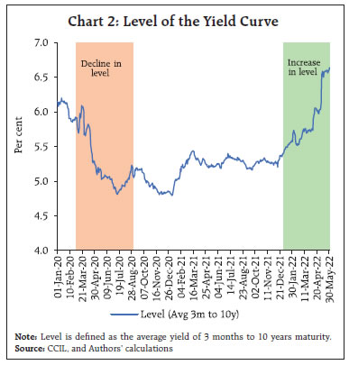
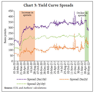
The government securities yield curve is widely regarded as a valuable predictor of future macroeconomic developments. Following the dynamic latent factor approach suitably modified to fit Indian conditions, this article uses a state space yield-macro model to show that in contrast to advanced economies, it is the level and curvature of the yield curve rather than its slope that contain useful information on market expectations about economic prospects and inflation expectations.

Introduction

Through 2021 and right up to the first half of 2022, government bond markets worldwide have experienced bouts of high turbulence. As elevated inflation pressures became persistent and broadened, monetary policy normalisation intentions were overtaken by front-loaded actions. As fear gained ground that inflation would remain stubborn due to supply disruptions exacerbated by the war in Europe, yields spreads – especially the difference between 10 year and 2 year yields or the ‘long-term spread’ – fell into negative territory in the US several times as if confirming that a recession was imminent. An animated debate has ensued, with detractors pointing to other yield gaps and ‘near-term forward spreads’ conveying no such early warning of an impending downturn in economic activity (Engstrom and Sharpe, 2022).

Market participants and the financial press have for long regarded the slope of the yield curve or the spread between long- and short-term yields as a valuable predictor of future macroeconomic developments. Economists have joined them since at least the early 1990s to show that it even outclasses indices of leading indicators and surveys of professional forecasters in its ability to scent future expansions and contractions (Mishkin,1990a; 1990b;1991; Estrella and Mishkin, 1996). Recent empirical evidence has been turned in to show that the predictive power of term spreads remains undiminished, and this statistical strength in predicting historical inflations and recessions over the year ahead is robust to the inclusion of additional predictors (Diebold and Li, 2006; Rudebusch and Wu, 2008). A contrarian view is that the presence of other factors such as liquidity and risk premiums make it tough to separate out ex ante real rates and expected inflation that are supposed to be embedded in the nominal interest rate (Patra et al., 2021a).

To the best of our knowledge, extracting the information content in the yield curve on macroeconomic prospects, which is essentially an empirical exercise, has not found much appeal in the Indian context. Hence, this article, which attempts to do so, needs to be regarded as exploratory. It uses a state space model which allows dynamic interaction between the yield curve, i.e., it’s level, slope and curvature, and relevant macroeconomic variables using a yield-macro model (as in Patra et al., 2021a) that follows the dynamic latent factor approach (Diebold et al., 2006) suitably modified to fit Indian conditions. The latent factor model considers two-way causality – components of the yield curve to macroeconomic variables and vice versa – so that potential bi-directional feedback from the yield curve to the economy and back are nested in the model (Diebold et al., 2006).

We find that in the Indian context, it is the level and curvature of the yield curve rather than its slope that contain useful information on market expectations about economic prospects and inflation expectations. The level of the yield curve has increased since 2021 after a steep decline during the pandemic. Furthermore, the yield curve is concave compared to 2019 levels, indicative of strengthening prospects for the recovery, higher inflation expectations and hence market expectations of front-loaded monetary policy normalisation.

The rest of the article is divided into three sections. Empirical evidence on the temporal movements in the yield and it’s latent factors are discussed in Section II. The estimation of the yield curve and its interlinkages with the macroeconomic variables of interest is set out in Section III. Section IV concludes with some forward-looking perspectives.

II. The Empirical Evidence

The yield curve depicts the interest rate path for different maturities of similar quality bonds. The long-term yield is a combination of the short-term interest rate set by the central bank, the expected future short-term interest rate embodied in the monetary policy stance, and the term premium – the difference between long-term and short-term yields.

Early explanations of the term premium were based on the expectations hypothesis under which the long-term interest rate is deemed to be the average of expected short-term rates over the maturity period of the bond (Fisher, 1896; Froot, 1989). Although simple, intuitive and elegant, empirical support for the expectations hypothesis is weak (Gürkaynak and Wright, 2012). In terms of the market segmentation hypothesis, on the other hand, long and short-term interest rates are not related to each other and should be viewed separately like items in different markets (Campbell, 1980). Investors have strong maturity preferences and they typically invest in their preferred maturity segment. Yields are determined by supply and demand forces within each market segment based on specific investor preferences in terms of durations, bond characteristics, and investment habits (Ang and Piazzesi, 2003). The criticism has been that this hypothesis can at best be used to explain any particular shape of the yield curve, but not the whole yield curve (Taylor and Masson, 1991; Gürkaynak and Wright, 2012). The preferred habitat theory – which is an extension of the expectations theory – postulates that investors generally prefer short-term bonds vis-a-vis long-term bonds, but they care about both expected returns and maturity. Since investors have different investment horizons based on their own preferences, they can only be incentivised to hold bonds other than their preferred maturity if adequately compensated for the additional risk through a premium i.e., higher interest rates. The liquidity premium theory is an offshoot of the expectations theory, but it places more weight on the risk appetite of market participants. Risk aversion causes forward rates to be higher than expected spot rates, usually increasing with maturity. Put differently, longer-term interest rates include a premium for holding longer maturities, which is the compensation demanded by the investor for the risk of illiquidity – tying up money for a longer period as well as price variability and relatively low marketability of longer-term securities.

Based on daily data for 2021-22 on trading volume in the government securities (g-sec) market in India, it is observed that 95.6 per cent of the total trading volume is in the residual maturity segment of up to 15 years (Chart 1).

For the period from March 2020 to May 2022 i.e., the pandemic period, the effective yield curve i.e., up to 15 years maturity, is segmented into various maturity buckets. Events which have a significant bearing on the shape of the yield curve are categorised as policy events and macroeconomic events. Specifically, monetary policy decisions and budget announcements constitute the policy events while GDP and inflation data releases are considered as macroeconomic events. The impact of each event is analysed through a 3-working day window prior to and post the event, which translates into a 7-day operating window. Spreads are considered for the following maturity segments: (i) 3 months and 2 years; and (ii) 2 years and 10 years, as they are the most liquid segments of the G-sec market (Table 1).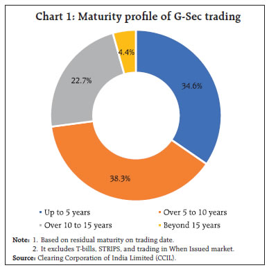

The measures announced on March 27, 2020 to counter the pandemic had a pronounced impact on the 2 years to 10 years maturity segment. Pandemic related measures significantly lowered the level of the yield curve (Chart 2). Short term rates plummeted, resulting in a steepening of the yield curve across various maturity segments (Chart 3).

The spread in the 3 months to 2 years segment increased by 8 bps on the policy day from the average of the previous three working days. The cumulative increase in the spread in the 2 years to 10 years segment was 35 bps (Table 1). Beyond 10 years maturity, however, the spread became flat, reflecting illiquidity. The surprise element in advancing the scheduled policy announcement from April to March 2020 amidst the nation-wide lockdown and an unprecedented rate cut of 75 bps accompanied by liquidity injections through targeted long term repo operations (TLTROs) and reduction in cash reserve ratio (CRR) undertaken by the RBI unsettled the market. The impact on spreads in the subsequent policy of May 22, 2020 when the policy repo rate was reduced by a further 40 bps was muted in comparison.

On January 8, 2021 when the RBI announced the reintroduction of the 14-day variable rate reverse repo (VRRR) auctions for rebalancing liquidity conditions, the market misinterpreted it as a precursor to policy tightening. Consequently, the spread in the 3 months to 2 years maturity segment steepened by 11 bps after the announcement (t+3) although the spread in the 2 years to 10 years segment moderated by 12 bps.

The announcement of the Union Budget on February 1, 2021 had a marginal impact on various segments – the spread in the 2 years to 10 years segment increased by 4 bps despite the announcement of a large market borrowing programme. Subsequently, the announcement of a secondary market G-sec acquisition programme (G-SAP) for Q1:2021-22 on April 7, 2021 assuaged market concerns and the yield curve flattened by 4 bps in the 2 years to 10 years maturity segment. The termination of the G-SAP programme on October 8, 2021 raised long term rates relative to those in the short term segment, thereby increasing the spread in the 2 years to 10 years segment. The announcement of the Union Budget for 2022-23 increased the spread of the 2 years to 10 years segment by 10 bps reflecting the unanticipatedly large borrowing programme of the government and India’s non-inclusion in the global bond indices, which resulted in a sharp spike in longer term rates.

With the announcement of the standing deposit facility (SDF) in April 2022 which came as a surprise to the market, the spread increased by 7 bps in the 3 months to 2 years segment, despite the floor of the liquidity adjustment facility (LAF) corridor (overnight SDF rate) being raised by 40 bps to 3.75 per cent. Similarly, the unexpected increase in the policy repo rate by 40 bps and the hike in CRR by 50 bps on May 4 increased the spread in the 3 months to 2 years segment by 7 bps; however, the impact on the 2 years to 10 years segment was moderate at 3 bps.

Turning to macroeconomic data releases, the monthly CPI inflation print is usually released on the 12th day of every month (unless it is a holiday). Prior to the release, professional forecasters’ median projections are characterised as a consensus forecast. Any noticeable positive divergence (actual more than consensus forecast) creates market unease, which generally gets reflected in the hardening of long term rates and steepening of the yield curve. In the Indian context, however, such surprises tend to have a mixed impact because of the interplay of such releases with monetary policy operations. For example, during the first COVID-19 wave (up to December 2020), inflation surprises increased the spread in the 2 years to 10 years segment (Table 2). Subsequently, however, such surprises resulted in an increase in the spread in the 3 months to 2 years segment as the RBI embarked on liquidity rebalancing, which was interpreted by the market as a reversal of the policy stance. Post October 2021, however, markets started factoring in higher inflation risks. The upward shift in the floor of the LAF corridor through introduction of the SDF in April 2022 increased the spread perceptibly at the short end.

This unequal increase in the spread in various segments has an impact on curvature – increasing the mid-segment of the curve more than the end-points and resulting in the hump shape of the curve getting more pronounced.

The latent yield curve factors provide vital information about future macroeconomic outcomes. To illustrate, Q1:2020-21 GDP growth, which provided the earliest official estimate of the impact of the pandemic, was released on August 31, 2020. Yield curve factors provided an early view of the imminent contraction even before the data release – a sharp decline in the level of the yield curve; little increase in the spread in the 3 months to 2 years segment, but a sharp increase in the 2 years to 10 years spreads, indicating that markets were expecting a recovery thereafter with expectations of continued monetary policy accommodation (Chart 3). During 2022 so far, increasing levels have co-existed with declining spreads, especially in the 2 years to 10 years segment. The spread between 3 months and 2 years yields increased, resulting in an increase in curvature (concavity) of the yield curve, indicative of an upbeat economic outlook amidst rising inflation expectations. The long term spread (between 3 months and 10 years yields) also declined sharply indicating expectations of monetary policy tightening, going forward.

In this background, curvature movements are illustrative of the evolving state of the economy and emerging developments. For example, the curvature underwent a significant decline as market liquidity and economic activity dried up with the onset of the pandemic (Chart 4). With the introduction of the COVID related measures, however, it reversed its trend and increased sharply during March to May 2020. The curvature again increased during the run up and announcement of the Union budget 2021-22, which unveiled a large market borrowing programme. This phase continued till the announcement of G-SAP in April 2021 which mollified market sentiments thereafter. This, along with the rapid surge of the second wave of COVID-19 infections, reduced the curvature significantly. Thereafter, the curvature continued with its uptrend till the announcement of policy rate hikes in May 2022 which raised short term rates much more in proportion to the medium term.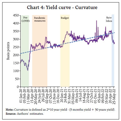

The empirically estimated yield curve factors¹ are dynamically cross-correlated with macroeconomic variables to identify lead-lag relationships (Chart 5). The results indicate that increase in economic activity measured by the output gaps and higher inflation are associated with an increase in the level of the yield curve and a reduction in the slope and curvature.

On the other hand, correlations of slope and curvature and macro-outcomes (economic activity, inflation) and the policy rate do not produce the expected results. This could be due to the fact that simple correlations ignore the complex underlying interlinkages. This deficiency can be overcome by using a yield-macro model adapted to India specific characteristics of the debt market to which we now turn.

III. Methodology and Results

In order to extract the macroeconomic signals contained in the yield curve, we use a state space model which allows dynamic interaction between the yield curve factors – level², slope³, and curvature⁴ – and the macroeconomic variables (Patra et al., 2021a)⁵. The estimation framework follows the tradition of the dynamic latent factor approach (Diebold et al., 2006), which augments the yield-only model with macroeconomic variables representing real activity, inflation, the monetary policy stance, global factors, liquidity conditions and the government market borrowing programme (Diebold and Li, 2006). For this purpose, g-sec yields with maturities of 3 months to 30 years for the period Q1:2011 to Q1:2022 are considered.

The model is estimated by using Bayesian methods with relatively weak priors (i.e., assuming the parameters to vary over a wide range rather than confined to a tight range as we are less confident of the value of the parameters a priori). Impulse responses are generated by using the identification followed in Diebold et al., (2006). The steady states are solved by applying a Newton-type algorithm. The unobservables (latent variables) are filtered out by using a smoothed Kalman filter.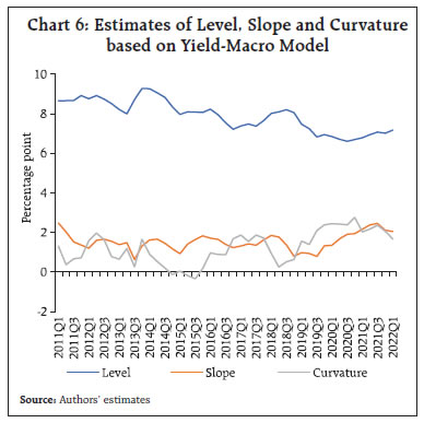

The estimated Lt, St and Ct from the model point to a steady softening of the level of yields from Q4 of 2018 till 2020, which indicates that the yield curve shifted downwards. Subsequently, the level has shown as upward movement. The slope of the yield curve was found to be increasing till mid-2021 and it remained at that level thereafter. The curvature too had shown an increasing concavity till 2020, but remained relatively stable subsequently. In Q1:2022, both slope and curvature were much above where they were during Q1:2019 (Chart 6).

Temporal changes in yield curve factors and the information in them regarding future macroeconomic developments can be explored by using impulse response functions (IRFs) from the yield-macro model (Chart 7). A positive surprise change in the level of the yield curve is followed by hump-shaped responses in slope and curvature. This implies that while initially yields of all maturities move up in lockstep, short-and medium-term maturities’ yields increase more than longer maturities in the subsequent quarters. An increase in the level factor points to rising economic activity, the policy rate and inflation. An increase in the level factor is equivalent to an increase in future expected inflation, which lowers the ex ante real interest rate. This boosts economic activity.⁹ The nominal policy rate rises in response to the level shock, which dampens the inflationary impact (Chart 7a).

An increase in the slope (30 years over 3 months) steepens the yield curve and is expected to be pointing to output gains. Contrary to the majoritarian view (Diebold, Rudebusch and Aruoba, 2006; Estrella and Mishkin, 1996), however, we could find only negligible responses of macro variables to shocks in the slope factor (Chart 7b). This suggests that, controlling for the level and curvature, changes in the slope are not very informative about future economic growth in India.

On the other hand, curvature provides interesting insights into future macroeconomic developments, in contrast to mainstream literature, which assigns an insignificant role to it (Diebold et al., 2006). The larger role of curvature vis-a-vis the slope in providing more information on future macroeconomic developments in an emerging market economy like India is attributed to the fragmentation of demand across maturity segments. For instance, the demand for long-term maturity bonds comes mostly from ‘buy and hold’ investors such as insurance companies and provident funds as the revenue streams from long-term g-secs are broadly aligned with their liability pattern. This leads to infrequent trading, resulting in low turnover in the medium to long segment compared to that of short to medium-term maturities. The higher demand for short to medium-term securities, particularly up to 10 years is reflective of active trading in managing portfolios, rendering them more responsive to evolving developments and expectations about macroeconomic outcomes. Thus, one would expect the mid-segment of the yield curve to be more sensitive to evolving developments, which would characterise the curvature as being more representative of market sentiments and expected outcomes than other latent factors.

A curvature surprise suggests a boost to economic activity for about 4 quarters and then a slow reversion sets in (Chart 7c). With the curvature shock, expected inflation rises in the medium term, triggering an increase in the policy rate which suppresses the actual inflation outcomes.

IV. Conclusion

The yield curve contains important clues on the likely behaviour of the economy, but a discerning assessment of the underlying latent factors is warranted, tempered by country-specific conditions and a methodological framework that allows for the dynamic interaction between the latent factors and key macroeconomic variables.

The empirical investigation we conduct here is focussed on India’s pandemic experience and interesting insights emerge. First, the slope of the yield curve steepened with the onset of pandemic-related policy easing. This trend has reversed in the recent policy tightening phase. Second, the declining level of the yield curve pointed to a contraction even before the data release in 2020-21. Third the curvature increased sharply during the pandemic-related easing and after the announcement of a large market borrowing programme for 2021-22 till the announcement of G-SAP in April 2021.

The results from a yield-macro model indicate that the level and curvature of the yield curve have more information content on future macroeconomic outcomes than the slope. This finding contrasts with the received wisdom and the experience of other countries. In sum, the yield curve is indicating an improvement in long-term growth prospects and an upshift in ex ante inflation expectations. At the same time, the fact that the yield curve has become steeper and concave reconfirms expectations of tighter monetary policy in the period ahead.

References

Ang, A., and Piazzesi, M. (2003). A no-arbitrage vector autoregression of term structure dynamics with macroeconomic and latent variables. Journal of Monetary Economics, 50(4), 745-787.

Campbell, T. S. (1980). On the extent of segmentation in the municipal securities market. Journal of Money, Credit and Banking, 12(1), 71-83.

Diebold, F. X., and Li, C. (2006). Forecasting the term structure of government bond yields. Journal of Econometrics, 130(2), 337-364.

Diebold, F. X., Rudebusch, G. D., and Aruoba, S. B. (2006). The macroeconomy and the yield curve: a dynamic latent factor approach. Journal of Econometrics, 131(1-2), 309-338.

Engstrom, E. C., and Sharpe, S. A. (2022). (Don’t Fear) The yield curve, reprise. FEDS Notes, March 25. Available at https://www.federalreserve.gov/econres/notes/feds-notes/dont-fear-the-yield-curve-reprise-20220325.htm.

Estrella, A., and Mishkin, F. S. (1996). The yield curve as a predictor of US recessions. Current issues in economics and finance, 2(7).

Fisher, I. (1896). Appreciation and interest. Publications of the American Economic Association, 11, 21-29.

Froot, K. A. (1989). New hope for the expectations hypothesis of the term structure of interest rates. The Journal of Finance, 44(2), 283-305.

Gürkaynak, R. S., and Wright, J. H. (2012). Macroeconomics and the term structure. Journal of Economic Literature, 50(2), 331-67.

Mishkin, F. S. (1990a). What does the term structure tell us about future inflation?. Journal of Monetary Economics, 25(1), 77-95.

____________ (1990b). The information in the longer maturity term structure about future inflation. The Quarterly Journal of Economics, 105(3), 815-828.

____________ (1991). A multi-country study of the information in the term structure about future inflation, Journal of International Money and Finance 19, March, 2-22.

Patra, M.D., Behera, H. and John, J. (2021a). A macroeconomic view of the shape of India’s sovereign yield curve. RBI Bulletin, Reserve Bank of India, June.

_______(2021b). Is the Phillips Curve in India Dead, Inert and Stirring to Life or Alive and Well?. RBI Bulletin, Reserve Bank of India, November.

Rudebusch, G. D., and Wu, T. (2008). A macro-finance model of the term structure, monetary policy and the economy. The Economic Journal, 118(530), 906-926.

Taylor, M.P. and Masson, P.R. (1991). Modelling the yield curve. IMF Working Paper, December.

* This article is prepared by Michael Debabrata Patra, Joice John, Krishna Mohan Kushwaha and Indranil Bhattacharyya of the Reserve Bank of India. The views expressed in this article are those of the authors and do not represent the views of the Reserve Bank of India.

¹ Level is equal to the average yield on all maturities; Slope is the difference between 30 years and 3 months yield; Curvature is 2 times 10 years yield minus the sum of 30 years and 3 months yields.

² Level is the average yield across maturity and usually co-move with equilibrium long rate.

³ Slope is defined as long-term rates minus short-term rates. Thus, an increase in slope means steepening of the yield curve. This notion is used throughout the article.

⁴ Curvature of the yield curve describes the relationship between yields at short, medium and longer maturities. Higher curvature means higher concavity of the curve i.e. the yield curve is steep in the short to medium tenure compared to medium to long-end yields and therefore shows a hump in the yield curve. This notion is used throughout the article.

⁵ The details of the model structure, estimation methodology and goodness of fit can be found in Patra et al. (2021a).

⁶ Source: Bloomberg.

⁷ Exponential decay describes the process of reducing an amount by a consistent percentage rate over a period of time.

⁸ Real activity is represented by the output gap (OG) (as estimated in Patra et al. 2021b), inflation (INF) by seasonally adjusted quarter on quarter changes in the CPI and monetary policy is proxied by the weighted average call money rate, the operating target of monetary policy. Liquidity conditions are captured by the outstanding absorption/injection under the Reserve Bank’s liquidity adjustment facility as a proportion to banks’ net demand and time liabilities or LIQU, government market borrowing is proxied by the market borrowing to market turnover ratio (GMB) and global uncertainty is represented by the Global Economic Policy Uncertainty index. The global factors are represented using the GEPU Index which is a GDP-weighted average of national EPU indices for 21 countries, each reflecting the relative frequency of own-country newspaper articles that contain a trio of terms pertaining to the economy (E), policy (P) and uncertainty (U). The data are available at https://www.policyuncertainty.com/global_monthly.html

⁹ An ex-post real interest rate does not appear to produce an equivalent response, as a positive shock to inflation does not boost economic activity (Diebold, Rudebusch and Aruoba, 2006).