This article investigates the relationship between external debt and growth with a view to identify the growth maximising threshold level of external debt for India. The empirical results suggest that as against India’s current external debt to GDP ratio of 20 per cent, the estimated threshold level is higher in the range between 23 per cent and 24 per cent of GDP, indicating space for attracting more debt flows of the order of USD 90 billion. Given the risk of amplifying external vulnerabilities because of higher exposure to external debt, the estimated space may be used carefully balancing the objective of growth and macro-stability. Introduction External debt, by supplementing domestic savings, can help countries grow faster. But a large stock of external debt can potentially create vulnerabilities and dent growth prospects. Since the onset of the pandemic, many countries have expanded public spending to support the recovery, which has led to a build-up of their external debt (IMF, 2022). For the low-and middle-income countries, excluding China, the ratio of external debt to GNI averaged 42 per cent in 2020, a 4.9 percentage point jump from 2019. Similarly, the external debt to exports ratio rose to 154 per cent from 126 per cent during the corresponding period (World Bank, 2022). Against this evolving global backdrop, this article investigates the relationship between external debt and growth in India and estimates growth maximising optimal threshold level of external debt by employing various models, such as spline regression, threshold regression and smooth transition regression, in addition to the quadratic regression. Rest of the article is organised into six sections. Section 2 outlines stylised features of India’s external debt in terms of historical and recent trends. Section 3 provides a brief review of literature. Section 4 presents the methodology and data, while Section 5 discusses the empirical results. Finally, Section 6 concludes. II. Stylised Features of India’s External Debt Historical Trends On the eve of Independence, India had little external debt. In the aftermath of independence, India adopted a planned era of economic growth and development anchored by Five-Year Plans with an overarching theme of import substitution through public sector attaining the commanding heights of the economy. India’s external debt rose from below 2 per cent of GDP at end-March 1955 to about 13 per cent by end-March 1970. The focus was to augment the economy’s investment rate by supplementing domestic savings with foreign borrowing and external transfers in the form of grants. During the 1970s, the external debt ratio remained range-bound in the neighborhood of just below 15 per cent. However, the widening of the current account deficit during 1980s was increasingly funded by the debt capital in the form of costly external commercial borrowings (ECBs), IMF loans and NRI deposits. Accordingly, the ratio of external debt to GDP rose to 38.7 per cent as at the end of 1991. A new policy on external debt came into being on the basis of the lessons emanating from the balance of payments (BoP) crisis of 1991 and the recommendations of the High-level Committee on Balance of Payments, 1993 (Chairman: Dr. C. Rangarajan). The new policy was guided by (i) restrictions on size, maturity and end-use of ECBs; (ii) LIBOR-based interest ceiling on non-resident deposits to discourage the volatile component of such deposits; (iii) pre-payment and refinancing of high-cost external debt; and (iv) measures to encourage non-debt creating financial flows such as foreign direct investment (FDI) and foreign portfolio investment (FPI). In the aftermath of the new policy, the ratio of external debt to GDP moderated significantly and consistently and reached around 17.0 per cent by the end of 2005. Even though it accelerated post 2005, the ratio remained low in relation to the levels witnessed in the early 1990s (Figure 1). The World Bank classifies external debt into long-term debt, short-term debt and IMF credit. The long-term debt is further broken down into public & publicly guaranteed debt (PPG) and private non-guaranteed debt (PrNG). In terms of share in the total external debt, the PPG accounted for over 80 per cent through the decades till 2000, barring 1980s. The PPG constituted basically borrowing from multilateral and bilateral sources. During the first half of 2000s, these high-cost multilateral and bilateral loans were prepaid as part of a conscious policy choice. Further, reliance on concessional borrowings from official creditors was pared down. As a result, the share of PPG halved from about 80 per cent in 2000 to about 38.0 per cent in 2006. As at the end of 2020, the share of PPG in total external debt stood at 34.2 per cent. On the other hand, as the process of reforms and liberalization rolled out during the 1990s, room for greater private corporate participation opened up, requiring modernization of the manufacturing sector by allowing greater access to foreign technology and foreign capital. Consequently, the share of PrNG rose to 46.0 per cent from about 15.0 per cent during the same period. As at the end of 2020, the share of PrNG in total external debt stood at 46.5 per cent (Figure 2). 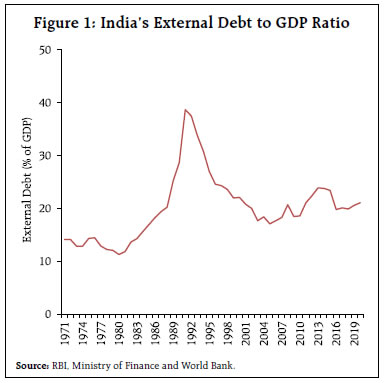 Another stylised feature discernible from a cross-country perspective involving low-and-middle-income countries is that countries with higher per-capita income are typically the ones with lower share of public & publicly guaranteed debt (Figure 3a) and higher share of private non-guaranteed debt in the total external debt (Figure 3b). In the case of India, the former ratio is below, while the latter ratio is above the cross-country trend line. This implies perhaps that among the low-and-middle-income-countries, India proactively, though in a carefully calibrated manner, encouraged private sector access to foreign debt capital, while exercising conservatism in providing public sector access to such capital. This policy approach to foreign debt within a broader policy on capital account convertibility has indeed served the country well.
Recent Trends On March 31, 2022, Department of Economic Affairs, Ministry of Finance, Government of India published India’s external debt statistics for the quarter ending December 2021. According to these estimates, India’s external debt stood at US$ 614.9 billion as at end-December 2022. Commercial borrowings (CBs) at US$ 226.4 billion, NRI deposits at US$ 141.9 billion and short-term trade credit at US$ 110.5 billion, together account for about 78 per cent of the total external debt (Figure 4). The external debt to GDP ratio as at end-December 2021 was 20.0 per cent. An analysis of the relative performance of India’s external debt in the aftermath of the pandemic/Great Lockdown (GLD) and the global financial crisis (GFC) reveals interesting insights. Outstanding external debt as at the end of the pre-crisis quarter is rebased to 100. Q2 of 2008 and Q4 of 2019 is identified as the pre-crisis quarter for the GFC and GLD, respectively. As can be seen from Figure 4, the total external debt, which fell below the pre-crisis levels in the immediate aftermath of the GLD, crossed the pre-pandemic levels as at end-December 2020 and consolidated further helped by NRI deposits crossing pre-pandemic levels as at end-June 2020; commercial borrowings crossing the pre-pandemic levels as at end September 2021; and short-term trade credit crossing the pre-pandemic levels as at end-December 2021. In contrast, India’s external debt remained relatively immune to the GFC reflecting the resilience of commercial borrowings, the most growth-sensitive and the largest component of India’s external debt. The resilience of commercial borrowings in the wake of the GFC stemmed largely from relatively muted impact of GFC on growth in sharp contrast to that during GLD (Figure 5). 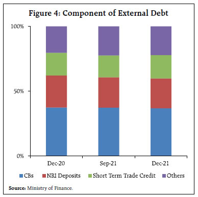 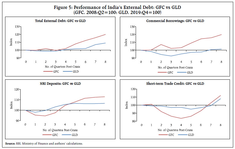 III. Literature Review In a typical neo-classical framework, for a country facing scarcity of capital, supplementing its domestic savings with external capital in the form of debt could fund larger investment, leading to higher economic growth. Some endogenous growth models have similar implications. Then, why does larger levels of accumulated external debt result in lower growth? There are two channels showcased in the literature: overhang and crowding-out. Debt overhang and crowding-out challenges arise when a country’s debt levels exceed its ability to repay in future, with the expected rise in debt service preempting the country’s output. In other words, returns on investing in the country which could have otherwise accrued to the investors would instead be taxed away by foreign creditors and as a consequence, new investment is discouraged (Krugman, 1988; Sachs, 1989). The channels via which adverse impact of external debt overhang and crowding out on growth could be realised are through lower volume of investment and efficiency of investment. In addition, uncertainty arising out of large debt stock could reduce investment, output, consumption and hours worked/employment (Moore, 2016; Basu & Burdick 2015; Leduc & Lie, 2016). There are models underscoring non-linear effects of debt on growth, through reduced investment and productivity of investment (Cohen, 1994). Non-linear models advocate existence of a Laffer curve type effect of debt on growth. Along the left (or on the good) side of the curve, increase in the stock of external debt is associated with higher growth through increasing investment and productivity. On the other hand, a rise in the stock of external debt on the right (or the bad) side of the curve would manifest in lower growth with reduced investment and productivity. The tipping/inflexion point of such an external debt Laffer curve is the growth-maximising threshold. There have not been many empirical studies on the impact of external debt on growth. In the empirical literature, typically a reduced form Barro-type growth model is employed, augmented with relevant external debt variables to capture the impact of external debt on growth. Further, these studies are basically cross-country in nature (Pattilo et al 2002, 2004, 2011; Clements, et al., 2003; Jayaraman et al 2009; Lau et al 2014; Siddique et al., 2016; Quareshi et al 2019; and Felix, 2020). Pattilo et al (2002, 2004, 2011) assess the non-liner impact of external debt on growth using a large panel data set of 93 developing countries over 1969-98. The findings support that while the average impact of debt becomes negative at about 30-40 per cent of GDP, the marginal impact turns negative at about half of the above range. Clements et al (2003) examine the channels through which external debt affects growth in 55 low-income countries covering the period 1970-99. The results indicate a threshold level of around 30-37 per cent of GDP. Siddique et al (2016) analyses the extent to which the external debt burden impacts growth, both in short-run and long-run, in 40 heavily indebted poor countries based on the data for 1970-2007. The results support the debt overhang hypothesis. Qureshi et al (2019) examines the relationship between the types of external debt (total, public and private external debt) and income growth using data for 23 countries from 1990 to 2015. While the total external debt appears to have a negative effect on growth rate at the generic level, it is positively related with income growth in lower and upper-middle-income countries. Further, public external debt negatively impacts economic growth for all countries, while the impact of private external debt is not statistically significant. Contrary to other studies cited above, the authors don’t find evidence of a common threshold level for external debt. Jayaraman et al (2009) used panel data for six Pacific Island Countries (PICs) covering a 17-year period of 1988-2004. The results underscore that while in the long-run there is no relationship between external debt and growth, in the short-run, external debt promotes growth. Lau et al (2014) examine the nexus between external debt and growth in 17 Asian countries during 1988 to 2006. The results provide evidence that external debt contributes to growth in these countries. Felix (2020) determines the influence of external debt on economic growth in the Economic Community of West African States (ECOWAS) using the data from 1990 to 2016. The results support that in the short-run, the threshold stood at 45 per cent, while in the long-run, it was at 42.5 per cent. Thus, apart from presenting a mixed picture, the empirical literature is mostly populated with cross-country studies, not amenable to country-specific implications. Methodologically, most of the empirical studies employ estimation methods based on instrument variables, fixed effects, system GMM, Panel Vector Auto Regressive (PVAR) model, or Auto Regressive Distributed Lag models. Against the aforesaid review of literature, the present study attempts to contribute to the sparse country-specific empirical literate, focusing on India, modeling non-linearity by employing spline regression for detecting regime change, supplemented by smooth transition regression. The methodological details are presented in the following section. IV. Methodology and Data Nonlinear Multivariate Regression: Drawing on the empirical literature reviewed above, a standard Barro growth model is augmented with a quadratic function debt variable to evaluate the impact of external debt on growth. where y is real GDP per capita income growth, X is a vector of control variables and Θ is their associated vector of coefficients; D is the external debt variable represented by external debt as a per cent of GDP, and u is an error term which is an independent and identically distributed (IID) with mean zero and variance σ2. The parameters are estimated based on ordinary least square (OLS) method. To have a robust estimate of the optimal threshold of external debt which maximises economic growth, various econometric approaches based on spline regression with two regimes, threshold regression model and smooth transition regression method which are based on structural break are considered in this article. Spline Regression Model: A spline regression model allows for changes in slope, with the estimated line being continuous and can consists of two or more straight line segments. Thus, the model is continuous, with a structural break. In this article, accordingly two segmented line is considered to estimate the threshold and is expressed as follows: After some manipulation, the following equation is obtained: where, D* represent the external debt threshold and I(D > D*) is an indicator variable taking the value 1 if D > D*, and 0, otherwise. Here the coefficient δ is measured in terms of the change in the slope from β1, to examine whether the change in the slope is significant or not. The significant of this change in slope at given threshold will indicate optimal threshold. In this article, the threshold along with other coefficients of the model are estimated using nonlinear least square (NLLS) method. Threshold Regression Model Threshold regression approach is employed by Sarel (1996) and Khan and Senhadji (2001) to estimate the inflation threshold in inflation-growth nexus model. Sarel (1996) runs a series of regression models for given threshold level and the optimal threshold is chosen based on maximum R-squared or minimum root mean square error (RMSE). However, Khan and Senhadji (2001) argued that since the threshold is unknown, it should be estimated along with other parameters of the model rather than the procedure suggested in Sarel (1996). The model suggested by Khan and Senhadji (2001) is used in this article to estimate the optimal threshold of external debt and is presented below. H0: β1 = β2 is tested against H1: β1 ≠ β2 for checking for the existence of optimal threshold. The model is estimated using nonlinear least square (NLLS) method. Smooth Transition Regression Model Most economic variables change regimes in a smooth manner, with transition from one regime to another taking some time. Smooth transition regression (STR) model allows for incorporating regime switching behaviour both when the exact time of the regime change is not known with certainty and when there is a short transition period to a new regime. Therefore, STR models provide additional information on the dynamics of variables that show their value even during the transition period. Further, smooth transitions between regimes are often realistic than abrupt switches. In this article, the model described in Espinoza et al. (2010) and Deepak et al (2011) is adopted with slight modification and is given below. G(.) stands for a continuous transition function usually bounded between 0 and 1. Most popularly used transition functions are logistic and exponential function and are defined as follows: The slope parameter γ > 0 is an indicator of the speed of transition between 0 and 1, whereas the threshold parameter c points to where the transition takes place, and the transition variable is denoted by d. In this article, both the logistic smooth transition regression (LSTR) as well as exponential smooth transition regression (ESTR) models are used. The parameters of the model including transition parameter and threshold are estimated using nonlinear least square (NLLS) method. The logistic specification of smooth transition is based on the cumulative logistic function, while the exponential specification if based on the inverted normal density function. This article uses annual data from 1970 to 2020 sourced basically from the Database on Indian Economy (DBIE), Reserve Bank of India1. However, wherever data is not available from RBI, such data is supplemented from the database of World Development Indicators, World Bank. V. Empirical Results To begin with, the real GDP per capita growth is plotted against the external debt to GDP ratio in Figure 6 to assess the relationship between them. There appears to be a nonlinear relationship between external growth and growth in India (Figure 6). In order to better understand the type of nonlinear relationship that exists between external debt and economic growth, and the sensitivity of inflexion point, a bivariate polynomial regression with various power functions including quadratic is investigated. The estimated coefficients of polynomial regression with various power along with their optimal external debt threshold is presented in Table 1 and the results are illustrated in Figure A.1 in Annex. The results from applying different functional forms show that the relationship between external debt and economic growth remains nonlinear (concave) and it depicts an inverted U-shaped relationship, corroborating the presence of a Laffer-curve type relationship. Higher power yields slightly higher optimal level of external debt2. The estimated optimal level of external debt estimated using different functional form is in the range of around 23.8 to 25.4 per cent. The optimal level of external debt estimated with power 2 is at 24.51 per cent. 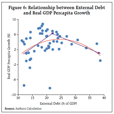
| Table 1: Sensitivity of Turning point of External Debt | | Power | Constant | Coeff. of External Debt | Coeff. of External Debt Power term | Optimal Point | | 1.2 | -15.20** | 5.02** | -2.22** | 23.77 | | (7.12) | (1.95) | (0.87) | | | 1.4 | -12.66** | 2.53** | -0.51** | 23.95 | | (6.17) | (0.98) | (0.20) | | | 1.6 | -10.77* | 1.71** | -0.16** | 24.14 | | (5.47) | (0.66) | (0.06) | | | 1.8 | -9.30* | 1.30** | -0.06** | 24.32 | | (4.94) | (0.50) | (0.02) | | | 2.0 | -8.12* | 1.05** | -0.02** | 24.51 | | (4.52) | (0.41) | (0.01) | | | 2.2 | -7.17* | 0.88** | -0.01** | 24.69 | | (4.181) | (0.343) | (0.003) | | | 2.4 | -6.38 | 0.77** | -0.004** | 24.87 | | (3.907) | (0.299) | (0.001) | | | 2.6 | -5.71 | 0.68** | -0.002** | 25.05 | | (3.679) | (0.266) | (0.001) | | | 2.8 | -5.14 | 0.61** | -0.001** | 25.23 | | (3.4888) | (0.2409) | (0.0003) | | | 3.0 | -4.65 | 0.56** | -0.0003** | 25.41 | | (3.3277) | (0.2213) | (0.0001) | | Note: (1) Figures in parentheses are the Standard Error.
(2) * indicates significance at 10%, ** significance at 5% and *** significance at 1%. | To have a robust estimate of the inflexion point, nonlinear multivariate regression is considered by including a set of control variables drawn from the literature such as log of real per capita income with a lag (initial level of per capita income)3, percentage change in the terms of trade, gross domestic investment as a per cent of GDP, openness indicator (exports plus imports as a ratio to GDP), population growth rate, enrolment rate in primary school, gross fiscal deficit of general government as a ratio to GDP, CPI-Combined inflation rate, total external debt service as a per cent of GDP and external debt indicator (external debt to GDP). The same set of control variables are included in other nonlinear models considered in this article. Initial level of per-capita (log of real per capita income) is expected to have a negative coefficient, drawing from income convergence hypothesis. Population growth and investment rate represent the conventional factors of production, while the primary school enrolment rate proxies for the quality of human capital. The coefficient on population rate is typically found to be negative in the empirical literature while that on investment and primary school enrolment are expected to be positive. The terms of trade variable is meant to capture external shock. For a commodity-importing country like India, coefficient on terms of trade is expected to be negative. The openness indicator is meant to reflect the strand in the literature that more open economies tend to have higher longterm growth in per-capita income. The fiscal balance variable accounts for the role of the fiscal in growth and the coefficient is expected to be positive. Inflation variable represents the impact of price rise on growth and hence expected to have a negative coefficient. As the data on external debt ratio and debt services ratio are available in DBIE from 1990-91 onwards, the data for these variables including enrolment in primary school prior to 1990-91 are collected from the World Bank. Nonlinear Multivariate Regression: Initially the nonlinear multivariate regression is estimated using all the control variables. However, population growth and gross fiscal deficit are found to be insignificant. Therefore, to have a more parsimonious model of estimating threshold, these two variables are excluded in further investigation as inclusion of these statistically insignificant variables may influence the estimation of other coefficients in the model, which in turn impact the estimated threshold. Ordinary Least Square estimation of the models exhibits presence of serial autocorrelation and heteroskedasticity. Therefore, these equations are estimated using the newey-west standard errors for coefficients estimated by OLS regression as newey-west standard error estimates are robust to heteroskedasticty and autocorrelation4. Results of the nonlinear multivariate regression excluding population growth and gross fiscal deficits are presented in Table 25. The initial income is statistically significant with negative sign supporting the conditional growth convergence hypothesis. Investment rate and the schooling enrolment rate too are statistically significant with positive sign, an empirical finding in line with the growth literature. The coefficient on terms of trade is negative and statistically significant, underscoring the fact that India is a commodity importing country. The coefficient on openness indicator is negative and statistically significant. Inflation coefficient has proper negative sign and statistically significant. The positive and statistically significant external debt (D) indicates that accumulation of external debt leads to higher growth up to a certain level and the negative statistically significant coefficient of external debt-squared (D2) shows that the stock of external debt results in lower growth beyond a threshold. Based on the coefficients of D and D2, the threshold level of external debt for India is estimated to be around 27 per cent of GDP6. | Table 2: Linear and Quadratic Effect of External Debt on Growth | | | Linear | Quadratic | | Constant | 38.264** | 42.941*** | | (7.893) | (6.140) | | Log(Income)t-1 | -7.681*** | -8.829*** | | | (0.911) | (0.980) | | Term of Trade Growth | -0.050** | -0.043*** | | (0.014) | (0.014) | | Investment Rate | 0.472* | 0.506** | | (0.243) | (0.244) | | Openness | -0.125 | -0.189** | | (0.039) | (0.049) | | Schooling | 0.396** | 0.394** | | (0.156) | (0.150) | | Inflation | -0.199*** | -0.168*** | | (0.036) | (0.034) | | (Debt Service/GDP) | 0.001 | -0.104*** | | (0.022) | (0.029) | | D | 0.021 | 0.858*** | | | (0.037) | (0.130) | | D2 | | -0.016*** | | | | (0.002) | Note: (1) Figures in parentheses are the Standard Error.
(2) * indicates significance at 10%, ** significance at 5% and *** significance at 1%. | Spline and Threshold Regressions: Using the spline and threshold regression model as described in the methodology, the existence of optimal threshold external debt is tested. The empirical results from the spline and threshold regression estimated using NLLS method are presented in Table 3. | Table 3: Estimated Turning Point of External Debt Ratio: Spline and Threshold Regression Models | | | Spline Regression | Threshold regression | | Constant | 46.595*** | 47.742*** | | (6.203) | (6.091) | | Log(Income)t-1 | -8.873*** | -8.990*** | | | (1.401) | (1.307) | | Term of Trade Growth | -0.042*** | -0.042*** | | (0.015) | (0.015) | | Investment Rate | 0.550** | 0.539** | | (0.259) | (0.266) | | Openness | -0.195*** | -0.198*** | | (0.043) | (0.051) | | Schooling | 0.400** | 0.403** | | (0.165) | (0.161) | | Inflation | -0.179*** | -0.180*** | | | (0.045) | (0.049) | | (Debt Service/GDP) | -0.073 | -0.089* | | (0.050) | (0.046) | | β1 | 0.273** | 0.297** | | | (0.122) | (0.118) | | δ | -0.057*** | | | | (0.017) | | | β2 | | -0.438*** | | | | (0.107) | | Threshold (D*) | 23.40*** | 23.60*** | | (5.057) | (2.736) | | Test (H0: β1 = β2) | | 16.72*** | | | (p = 0.0002) | Note: (1) Figures in parentheses are the Standard Error.
(2) * indicates significance at 10%, ** significance at 5% and *** significance at 1%. | The significance of slope change in both the spline and threshold regressions suggest that there is a structural break in the external debt-growth relationship. The estimated threshold of external debt from spline and threshold regression is at 23.4 per cent and 23.6 per cent, respectively. This provides evidence that the impact of external debt on growth changes when external debt to GDP ratio crosses 23.4 to 23.6 per cent. Smooth Transition Regression: The empirical results from the smooth transition regression using both logistics and exponential transition function are presented in Table 4. The threshold of external debt estimated from logistic smooth transition regression (LSTR) and exponential smooth transition regression (ESTR) is at 23.5 per cent and 23.6 per cent, respectively. The findings from the LSTR and ESTR support the threshold estimated from the spline and threshold regression. The transition of the external debt-growth relationship from one regime to another at estimated threshold level based on the logistic and exponential transition function is illustrated in Figure 7. | Table 4: Estimated Turning Point of External Debt Ratio Based on Smooth Transition Regression (STR) | | | Logistic STR | Exponential STR | | Constant | 48.263*** | 42.567*** | | (5.346) | (6.325) | | Log(Income)t-1 | -9.021*** | -8.273*** | | | (1.330) | (0.741) | | Term of Trade Growth | -0.047*** | -0.058*** | | (0.012) | (0.013) | | Investment Rate | 0.547** | 0.546* | | (0.262) | (0.314) | | Openness | -0.191** | -0.154** | | (0.044) | (0.066) | | Schooling | 0.402** | 0.404** | | (0.172) | (0.178) | | Inflation | -0.189*** | -0.227*** | | | (0.042) | (0.048) | | (Debt Service/GDP) | -0.072 | 0.009 | | (0.046) | (0.046) | | β1 | 0.257*** | 0.160*** | | | (0.116) | (0.008) | | β2 | -0.117** | -0.149*** | | | (0.043) | (0.026) | | γ | 58.150 | 7.233 | | | (2159) | (6.714) | | Threshold (D*) | 23.49*** | 23.57*** | | (3.637) | (0.022) | Note: (1) Figures in parentheses are the Standard Error.
(2) * indicates significance at 10%, ** significance at 5% and *** significance at 1%. | The trend behaviour in the relationship between external debt and growth based on the above models are presented in Figure A.2 of Annex. The regime change and the threshold level are discernible from the spline regression, threshold regression and smooth transition regression as they are based on the structural break. On the other hand, the trend of the non-linear quadratic multivariate regression is smoother, making it relatively difficult to identify the threshold. The quadratic polynomial may not perhaps be the suitable representation of a nonlinear relationship, given that threshold estimates are sensitive to the form of nonlinear function included in the model and their estimated coefficients as seen in Table 1. Based on the thresholds emanating from the above structural break models, it could broadly be inferred that the growth maximising external debt to GDP ratio (optimal threshold) for India could be between 23.4 per cent and 23.6 per cent7,8. VI. Conclusion The article examines the relationship between external debt and economic growth in India. It finds evidence that there is a nonlinear relationship between them within a conventional conditional growth convergence framework, reflecting a typical inverted U-shaped external debt Laffer curve. The inflexion point or the growth-maximising external debt to GDP ratio threshold is estimated in the range of 23.4 per cent to 23.6 per cent. The actual external debt to GDP ratio as at end-December 2021 is estimated at 20 per cent, indicating a potential space to promote growth enhancing external debt by about 3 percentage points of GDP, equivalent to additional US$ 90 billion of debt at the current level of India’s GDP. India’s debt market is being progressively opened up to the foreign capital in a careful and calibrated manner. As part of the annual budget in 2020, the government announced a list of government securities that are fully opened to foreign investors without a limit under Fully Accessible Route (FAR). The Statement on Developmental and Regulatory Policies announced by the RBI on February 10, 2022 enhanced the investment limit under the Voluntary Retention Route (VRR) by ₹1 lakh crore. Further, efforts are underway for a possible inclusion of Indian G-sec in global bond indices. There are estimates that such an inclusion would prompt additional bond inflows into the Indian debt market, given the bourgeoning size of the FAR securities. These policy developments may be seen in the context of the findings of this study. At present, a rule-based dynamic limit for outstanding stock of ECBs at 6.5 per cent of GDP is in place. As India aims at higher, sustainable and inclusive growth, the need for attracting larger external debt flows within the estimated threshold may be assessed along with other external vulnerability parameters so that the growth objective is pursued while preserving overall macro-stability. References Basu, Susanto and Bundick Brent. 2017. “Uncertainity stocks in model of effetive demands.” Econometrica, Volume-85, No-3. 937-958. Clements, B., Bhattacharya, R., & Nguyen, T. 2003. “External debt, public investment, and growth in low-income countries.” IMF (IMF Working Paper No.249, WP/03/249). 249. Cohen, D. 1993. “Low investment and large LDC debt in the 1980’s.” American Economic Review. 437-449. Espinoza, R.,Leon, H., & Prasad, A. 2010. “Esatimating the Inflation-Growth Nexus - A Smooth Transition Model.” IMF Wroking Papers, WP/10/76. Jayaraman, T.K., & Lau, E. 2009. “Does external debt lead lead to economic growth in Pacific Island countries.” Jounal of Policy Modelling, 31, 272-288. Khan, M.S., & Senhadji, A.S,. 2001. “Threshold effects in the relationship between inflation and growth.” IMF Staff Papers, SP/01/48 1-21. Krugman, P. 1987. “Financing vs. forgiving a debt overhang: some analytical notes.” Journal of Development Economics, 29, 253-268. Lau, E., & Thain-Ling, K. 2014. “External Debt, Exports.” Journal of Applied Sciences 14 (18) 2170-76. Patillo, C., Poirson, H., & Ricci, L. A. 2011. “External debt and growth.” Review of Economics and Institutions 2 (3). Patillo, C., Poirson, H., Ricci L.,. 2004. “What are the channels through which external debt affects growth?” IMF (IMF Working Paper No-WP/04/15). Patillo, C., Poirson, H., Ricci, L.,. 2002. “External debt & growth.” IMF (IMF Working Paper No-WP/02/69). Qureshi, Irfan and Liaqat, Zara. 2020. “The Long-term consequences of external debt: Revisiting the evidence and inspecting the mechanism using panel VARs.” Journal of Macroeconomics. 63. Sachs, J.D.,. 1989. Developing country debt and economic performance. Volume 1. Chicago: University of Chicago Press. Sarel, M. 1996. “Non-linear effects of inflation on economic growth.” IMF Working Staff Papers, WSP/96/43 199-215. Schclarek, A.,. 2004. “Debt and economic growth in developing and industrial countries.” Lund University Department of Economic, 34 Working Paper,. Siddique, Abu, Selvanathan, E.A. and Selvanathan, Saroja. 2016. “The impact of external debt on growth: Evidence from highly indebted poor countries.” Journal of policy modeling 38 874-894. Sylvain, Leduce and Liu, Zheng. 2015. “Uncertainty shocks are aggregate demand shocks.” Federal reserve bank of san franscisco working paper 2012-10. WP/12/10.
Annex
|