Forward looking surveys on household sentiments are commonly used as leading indicators of economic conditions. This article focuses on the Consumer Confidence Survey for India. It examines the efficacy of the Survey parameters in forecasting some key macro-economic indicators, such as the Gross Domestic Product (GDP) growth and inflation. The article reveals that the survey contains useful leading information about economic conditions. In particular, it is observed that consumers’ expectations about prices and general economic conditions have a reasonable ability to predict consumer price inflation. Introduction Consumer confidence is regarded as a common leading indicator on the prevailing economic conditions as well as their future outlook by central bankers and researchers alike (Greenspan, 2002; Dees and Brinca, 2013). The Organisation for Economic Cooperation and Development (OECD) defines consumer confidence as an indicator of future developments of households’ consumption and saving based on their expectations about the financial and general economic situation, unemployment and savings, and considers it to be a leading indicator on the current economic situation as well as an early warning about the future turning points in the state of the economy (OECD, 2019). Both advanced and emerging economies conduct regular consumer surveys, while customising these surveys to suit their local needs. To illustrate, in the US, the University of Michigan has been the pioneering organisation conducting monthly Survey of Consumers in the US and compiling the Index of Consumer Expectations. The focus of the index is three pronged viz., the household prospects about their own financial situation, their opinion about the general economy in the near term, and their outlook about the general economy for the long term. Additionally, it also compiles an Index of Current Economic Conditions. The index gathers households’ perception of their own current financial situation vis-à-vis a year ago and their assessment of whether the present times are suitable for major household expenditures, such as expenditure on furniture and consumer durables, among others. Similarly, the Consumer Confidence Survey of the European Commission garners households’ responses on survey parameters, such as financial situation, general economic situation and spending, both for the previous and the ensuing year. Among emerging economies, the Bureau of Economic Research of South Africa is responsible for conducting the consumer survey since 1975. The final confidence index, derived by the Bureau, is a combination of the responses on expectations about the performance of the economy, expected financial situation of households and suitability to buy durable goods. Similarly, in Brazil, the Index of Consumer Confidence, compiled by the Federaçao do comercio do Estado de São Paulo (FCESP), is based on the consumers’ perceptions of their financial condition, their future prospects and the general economic conditions. Bank Indonesia too conducts a monthly consumer survey to gauge consumer confidence in the economy. While the general utility of the consumer confidence surveys in providing leading information on economic conditions is well-accepted, this article goes a step further and attempts a statistical evaluation of the efficacy of such surveys in forecasting economic conditions in the Indian context. The article begins with a brief literature review on the inter-relationship brought out by studies from various economies between consumer sentiments and macroeconomic parameters in Section 2. It then provides a detailed discussion on the Consumer Confidence Survey of the Reserve Bank in Section 3, followed by the details on the empirical methodology adopted in the article for establishing the interlinkage between consumer outlook and economic conditions in Section 4. The results from empirical exercise are discussed in Section 5 with conclusions in Section 6. 2. Literature Review The empirical literature on the inter-relationship between consumer sentiment indicators and macroeconomic parameters is fairly rich, with studies on this subject available from both advanced and emerging economies. Mendicino and Punzi (2013) employ a Vector Autoregression (VAR) model to study the impact of consumer confidence on macroeconomic variables, such as inflation rate, nominal interest rate, as well as measures of economic activity, including industrial production and unemployment rate for Portugal. Their results suggest that an unexpected increase in consumer confidence raises industrial production and pushes up the inflation rate. Similarly, sudden improvements in consumer sentiments leads to decline in unemployment rate. The significance of consumer confidence for predicting consumption spending has also been analysed for the US and the Euro area (Dees and Brinca, 2013). The authors utilise the University of Michigan’s Consumer Sentiment Index for the US and the index constructed by European Commission for the Euro area from 1985 to 2010 at quarterly frequency. Employing again a VAR framework, the results show that the consumer confidence indices can be, under certain conditions, good predictors of consumption expenditure. A time-series relationship between investor sentiments and stock returns has been explored, using consumer confidence as a measure of investor optimism, by Lemmon and Portniaguina (2006) for United States based on University of Michigan and Conference Board Survey of consumer confidence. The study reveals that consumer confidence has forecasting power for the returns on small stocks and future economic activity. A rich cross-country data panel has been used by Golinelli and Parigi (2004) to assess the validity of consumer sentiment indices in anticipating the evolution of economic activity. Their panel extends to eight countries viz., Australia, Canada, France, Germany, Italy, Japan, UK and USA over a period of about 30 years. Applying co-integrated VAR structure and considering a common set of variables for all countries, their findings suggest that consumer confidence cannot be simply summarised based on common macro-economic variables. Moreover, they show that consumer confidence indices have an ability to forecast economic activity, provided that their coincident nature is taken into account. The Consumer Confidence Survey (CCS) of the Reserve Bank captures information about various demographic characteristics of respondents, including their occupations. An examination of whether households’ assessment and expectations about their general economic situation is contingent on their occupation was attempted by Kumar et al. (2019). Applying an ordered logistic regression, the authors showed that opinions about general economic conditions do not vary across occupation groups. 3. Data We have used the quarterly data of the CCS from June 2010 to December 2018 (35 quarters).1 The CCS elicits households’ responses on five parameters viz., general economic situation, employment scenario, price level, household income and spending. The respondents’ views on both current situation as compared to a year ago, and the future outlook over a one-year period are solicited. Responses are solicited on a three-point scale, viz., improve/ will improve, worsened/ will worsen and remained/ will remain same. The aggregate sample size for each survey round is about 5,400 households. The details of the survey are elaborated in Annex A. As the study focuses on forecasting ability of households’ outlook, the net response2 (NR) for one year ahead expectations regarding the various survey parameters is used in addition to the Future Expectations Index (FEI)3. The macro-economic variables used in this article include the rates of growth of GDP and Private Final Consumption Expenditure (PFCE) (both at current prices) as obtained from the National Statistical Office (NSO). Additionally, the quarterly average of CPI (Urban) inflation rate, as available from Ministry of Statistics and Programme Implementation (MOSPI), is also considered. The CPI (Urban) has been chosen instead of CPI (Combined) as the CCS, at present, covers only urban areas. 4. Methodology Similar to the studies discussed earlier, we employ the VAR framework to analyse the impact of households’ expectations about the survey parameters4 on changes in our macro-economic variables and vice versa. The VAR(p) can be represented as: Consumer outlook variables and macro-economic indicators comprise the set of endogenous variables. Separate VAR formulations have been devised for each consumer outlook variable to examine its forecasting significance. Impulse response functions trace the reaction of current and future values of endogenous variables to a one-time external shock. Impulse responses were generated only for select cases, where survey variables were found to be significant. The various VAR formulations are described in Table 1 (Annex B). The common set of macro variables studied for the CCS parameters, except for household spending and employment outlook, are GDP growth rate and CPI(U) inflation. As household spending is more closely related to consumption expenditure, PFCE growth has been chosen in addition to GDP growth rate for spending outlook. Also, since it is generally observed that levels of economic activity and employment are closely associated, only GDP growth rate has been selected while examining responses for employment. 5. Empirical Evidence 5.1 Stylised Facts Before embarking on the discussion of the results from the empirical analysis, we bring out certain stylised facts about the representativeness of the CCS. First, we analyse the respondents’ profile for select past rounds (Chart 1 in Annex B). It is evident that the distribution of households has been largely similar over these rounds. A majority of respondents (around 90 per cent) belong to the age group of 22 to 59 years. There is no significant gender variation across these rounds, with male and female respondents being equally represented. Majority of the households participating in the Survey have income of Rs. 3 lakh or below. The family size for most of the respondents ranges between three and four. Homemakers lead the survey respondents followed by employed (salaried) and self-employed categories. Secondly, the respondents’ distribution is validated using data from Census 2011. Broadly, the distribution of sampling units matches the Census 2011 distribution for various demographic factors, as depicted in Chart 2 (Annex B). Thirdly, Chart 3 (Annex B) traces changes in FEI along with other macro-economic variables, helping us to correlate it with some of the major economic developments. Post-December 2016, the FEI has been above 120, reaching a peak of 129 in December 2017 that seems to portray the upbeat outlook of households on account of demonetisation. Over the last few rounds, GDP and PFCE growth rates are found to be co-moving. Moreover, it is observed that inflation has been consistently below 6 per cent mark since December 2014. 5.2 Coherence5 - General Economic Situation vis-à-vis Other Indicators The future General Economic Situation (GES) may portray a combination of underlying factors. Therefore, it may be insightful to ascertain the parameter(s) that may influence consumers’ expectations about future GES the most. Accordingly, coherence of expectations about future GES with expectations about other indicators are depicted in Table 1. It is observed that the outlook on employment has been the key driver for future GES; it is followed by the outlook on households’ income, which has been consistently the second-most coherent driver of future GES. The Spearman rank correlation coefficient depicts the strength and direction of correlation between two ordinal variables. Similar to the coherence outcome, the Spearman rank correlation coefficient between employment responses with GES expectations too is seen to be the highest and statistically significant (Table 2 in Annex B). Employment responses are followed by income responses, which too share a positive and significant relation with GES. Outlook on spending is observed to have negative association (although low) with future GES for certain survey rounds, suggesting that higher spending is associated with pessimism about future GES. | Table 1: Coherence of Expectation on General Economic Situation vis-à-vis Other Indicators | | (Percentage of respondents) | | Round | Employment | Price | Spending | Income | | Sep-2016 | 55.4 | 23.0 | 53.9 | 54.6 | | Dec-2016 | 59.6 | 27.6 | 57.5 | 57.6 | | Mar-2017 | 62.6 | 33.6 | 49.3 | 49.8 | | Jun-2017 | 64.8 | 36.9 | 47.7 | 51.5 | | Sep-2017 | 67.0 | 33.4 | 47.9 | 52.6 | | Dec-2017 | 66.0 | 29.8 | 51.0 | 53.0 | | Mar-2018 | 64.8 | 34.3 | 47.7 | 50.8 | | Jun-2018 | 64.6 | 32.6 | 48.3 | 52.4 | | Sep-2018 | 68.9 | 36.3 | 48.4 | 49.4 | Apart from capturing households’ outlook on various pertinent economic aspects for next 12 months, the CCS also gathers their perceptions about the current economic scenario vis-à-vis previous year. In this context, it may be useful to understand the key drivers of current GES. With this objective, both coherence and Spearman rank correlation tests have been performed for current GES. The coherence results again highlight employment to be the most important driving factor for current GES (Table 2). Spearman correlations also show that the responses on current employment scenario are highly correlated (with a positive sign) with current GES (Annex B - Table 3). Household income level turns out to be the second-most important variable determining current GES. In sum, the perceptions about the current and expectations about the future GES are more aligned with those of employment scenario followed by household income. | Table 2: Coherence of Assessment on General Economic Situation vis-à-vis Other Indicators | | (Percentage of respondents) | | Round | Employment | Price | Spending | Income | | Sep-2016 | 47.9 | 31.2 | 44.3 | 44.7 | | Dec-2016 | 48.3 | 33.8 | 41.9 | 44.4 | | Mar-2017 | 53.2 | 42.6 | 35.3 | 43.4 | | Jun-2017 | 54.7 | 43.7 | 34.0 | 42.9 | | Sep-2017 | 56.6 | 42.1 | 35.5 | 43.5 | | Dec-2017 | 55.5 | 39.3 | 36.8 | 44.2 | | Mar-2018 | 55.1 | 44.7 | 34.8 | 43.1 | | Jun-2018 | 56.5 | 44.0 | 35.2 | 43.0 | | Sep-2018 | 59.1 | 45.4 | 33.2 | 41.2 | 5.3 CCS Indicators vis-à-vis Macroeconomic Indicators - Forecasting Ability To analyse the forecasting ability of CCS parameters, we plot the rolling correlations over a two-year period6 between net responses (NR) on CCS indicators and macro-economic indicators. The rolling correlations have been calculated for two-year window to assess the dynamic relationship between the variables. Also, a two-year window helps to reduce the impact of any shock/structural change in the component series. The rolling correlations reveal – -
a positive correlation for both NR on current and future GES with GDP growth rate, especially since September 2016; this, however, has declined in the recent period (Annex B - Chart 4a); -
a mixed picture in respect of correlation between NR on employment scenario and GDP growth rate – To illustrate, improving correlations with NR on current employment scenario and declining correlations with NR on future employment scenario, more so in the recent rounds (Annex B - Chart 4b); -
inverse correlations between the NR on price and CPI(U) during the period from 2013 to 2016 (Annex B - Chart 4c); -
broadly, a positive correlation between NR on current household income and GDP growth rate, particularly since 2015 (Annex B - Chart 4d); -
negative correlation between NR on future spending and CPI(U) inflation for most part of our study period, although it has turned positive in the recent period (Annex B Chart 4e). We investigate the Granger causality among the various pairs of variables. Granger causality enables to examine whether the joint lags of a variable are able to improve the overall estimation result. As our focus is to explore the possible impact of CCS expectations on macro indicators, we assess whether the various components of CCS are able to Granger cause relevant macro indicators. We apply the Toda and Yamamoto (1995) methodology, which is appropriate wherein variables may probably be integrated. The results of the Granger Causality reveal some cases wherein the impact of CCS variables is statistically significant (Annex B - Table 4). First, both price and GES responses of consumers seem to have forecasting information for inflation. Secondly, consumption expenditure seems to be driven by spending expectations. Thirdly, employment outlook has some impact on GDP growth rate. As variables in our analysis are I(1)7, Johansen Cointegrating test is performed for all specifications to examine if there exist any cointegrating relationship. It is found that in most of the cases there is no indication of any cointegration amongst the variables. So, we choose an unrestricted VAR wherein both CCS and other macro variables are included with first difference. VAR framework is modeled to assess the interplay of consumer sentiments on various indicators, including the relevant macro-economic factors. An appropriate lag specification of consumer NR series is selected in all VAR models such that it provides a better fit. Deeper lags imply more time may be required for transmission of the impact of consumer expectations to economic variables, whereas shorter lags imply quicker transmission. The VAR8 results indicate that the FEI does not have a significant relationship with both GDP growth and inflation (Annex B - Table 6). NR on price outlook has a statistically significant and negative impact on CPI(U) inflation (Annex B - Table 7). The result implies that an improvement in public outlook about prices results in easing of consumer inflation with a lag. Generally, food prices are a major concern for households, which may even play a major role in the formation of their future price and inflation expectations. Accordingly, the influence of future price NR on consumer food price inflation is also analysed (Annex C). As found earlier for price NR and CPI(U) relationship, the results reveal a significant impact of price outlook on food prices based on urban Consumer Food Price Index (CFPI(U)) inflation. The outcome underlines the strong influence of price expectations on food inflation in due course of time. It establishes the robustness of the result obtained earlier based on VAR estimation result of price NR with economic parameters. Similarly, NR on future GES has a strong and inverse influence on CPI(U) inflation (Annex B - Table 8). A positive and significant impact of the spending outlook is evident both on GDP and PFCE growth rates (Annex B - Table 9 & Annex B - Table 10 respectively).9 However, consumer outlook regarding future household income and future employment scenario do not seem to have a significant effect on economic variables (Annex B - Table 11 & Annex B - Table 12 respectively). Impulse response function (IRF) traces the impact of one-time shock in one parameter on the current and future values of other variables. It is noted that the AR roots lie within unit circle, which is a vital diagnostic for the stability and validity of IRF (Lutkepohl, 2005). Similar to outcome from VAR, it is seen that a unit standard deviation (SD) positive shock (beneficial price regime) to NR on price outlook leads to a slight decline in growth rate, which is statistically insignificant (Annex B - Chart 5). On the other hand, a favourable shock to NR on price outlook leads to decline in CPI(U) inflation. Likewise, a unit SD positive shock in future GES has a positive impact on CPI(U) inflation (Annex B - Chart 6). A shock to NR on future spending has a beneficial impact on GDP growth, although it is not significant (Annex B - Chart 7). A similar impact is seen on PFCE growth as a result of the shock to NR on future spending (Annex B - Chart 8). Proceeding further, the variance decomposition of each VAR formulation is carried out, as already enumerated in Table 1 (Annex B). The variance decomposition is a useful tool to understand the quantum, speed of adjustment and persistence due to a stochastic innovation in the system. The variance decomposition results for FEI is depicted in Chart 9A (Annex B). The results show that only 10 per cent of variation in GDP growth rate is explained by FEI by third quarter, which remains largely static over the rest of the period. The role of FEI is observed to be negligible in explaining the variation in inflation. More than 30 per cent of deviation in inflation is attributable to consumer price expectations by the second quarter, which shows a rising trend till the fifth quarter and stabilises thereafter (Chart 9B in Annex B). Although, household price expectations have a miniscule contribution in describing GDP growth rate, Chart 9C (Annex B) shows that more than 20 per cent variation in inflation is explained by public perception about the general economic conditions by the third quarter, which is quite similar to that obtained for price expectations. Charts 9D (Annex B) and 9E (Annex B) focus on the influence of spending outlook on GDP and PFCE growth rates, respectively. In both cases, the influence of consumer expectations takes three quarters to reach their respective highest points. Nearly 20 per cent of divergence is explained by spending responses for GDP growth rate, while the explanatory power for consumption expenditure is relatively low. Roughly, only 4 per cent of variation in GDP growth is attributable to consumers’ response for income (Annex B - Chart 9F). The impact of employment expectations on economic growth rate is seen to be trivial (Annex B - Chart 9G). | Table 3: Root Mean Square Error | | Macro variable | Baseline Random Walk | Price NR | GES NR | Spending NR (GDP) | Spending NR (PFCE) | | | [1] | [2] | [3] | [4] | [5] | | GDP growth rate | 1.71 | 2.72 | 2.97 | 3.32 | --- | | PFCE growth rate | 2.02 | --- | --- | --- | 2.82 | | CPI(U) inflation | 0.83 | 0.33 | 1.34 | 0.76 | 0.78 | The out-of-sample evaluation of VAR forecasting results has been performed with a baseline random walk10. For comparison, economic indicators till 2017 have been considered. Thereafter, forecast evaluation is performed for next four data points based on the root mean square error (RMSE). VAR regressions were re-run for the sub-sample period, i.e., June 2010 to December 2017, in addition to simple random walk. The RMSE based on four quarters of the next year are tabulated in Table 3 for various models. It is evident that the multivariate VAR framework provides considerable gains in inflation forecasting for models [2], [4] and [5] as the RMSE of said models is less than the baseline random walk. Apart from the VAR framework, as indicated above, the impact of outlook on prices, controlling for ‘inflation targeting’, on CPI(U) based inflation has also been examined using a single equation regression. The details are provided in Annex D. The results corroborate a decline in CPI(U) inflation with the improvement in consumer expectations about price after controlling for the inflation targeting regime. Summing up, it is found that net responses on price, GES and spending have valuable information about the future trajectory for CPI(U), GDP and PFCE growth rates. These results for India are not isolated; such outcomes are echoed in other studies as well.11 6. Conclusion The study examines if the CCS indicators have any forecasting ability with respect to major macro-economic indicators. The findings suggest that consumers’ outlook on price and general economic situation has significant forecasting power for inflation (CPI(U)). The NR on households’ overall spending has a positive and significant impact on both GDP and PFCE growth rate. It may be mentioned that the strong impact of price outlook can be corroborated using consumer food price inflation data also. However, the statistical results presented in this article may be considered as indicative, due to a limited sample size. Future research can build on the research presented in this article using a larger information set. References Bank Indonesia (2016), Metadata, Consumer Expectation Survey, URL: https://www.bi.go.id/en/statistik/metadata/survei/Documents/1-Metadata-Consumer-Survey-2016.pdf (Accessed on 03 April 2019). Bureau of Economic Research (2018), “Changes to the BER consumer survey”, URL: https://www.ber.ac.za/Knowledge/pkDownloadDocument.aspx?docid=9331 (Accessed on 03 April 2019). Christiano, L. J., Eichenbaum, M and Evans, C (1997), “Monetary shocks: what have we learned, and to what end?”, Handbook of Macroeconomics (Eds.: Woodford, M.). Elsevier, Amsterdam, pp.65-148. Dees, S. and Brinca, P.S. (2013), “Consumer confidence as a predictor of consumption spending: Evidence for the United States and the Euro area”, International Economics, 134, pp.1-14. Golinelli, R. and Parigi, G. (2004), “Consumer sentiment and economic activity”, Journal of Business Cycle Measurement and Analysis, 2004(2), pp.147-170. Greenspan, A. (2002), “Remarks to the Bay Area Council Conference.” San Francisco, California, January 11; Available at http://www.federalreserve.gov/boarddocs/speeches/2002/20020111/default.htm. Kumar, N., Mishra, A. and Singh, D.P. (2019), “The Consumer Rules! Some Recent Survey-based Evidence”, RBI Bulletin, April 2019, pp.117-131. Lemmon, M. and Portniaguina, E. (2006), “Consumer confidence and asset prices: Some empirical evidence”, The Review of Financial Studies, 19(4), pp.1499-1529. Lutkepohl, H. (2005), “New Introduction to Multiple Time Series Analysis”, New York, Springer. Mendicino, C. and Punzi, M.T. (2013), “Confidence and economic activity: the case of Portugal”, Economic Bulletin and Financial Stability Report Articles, Banco de Portugal, pp.39-49. OECD (2019), Consumer confidence index (CCI) (indicator).doi: 10.1787/46434d78-en (Accessed on 03 April 2019). Toda, H.Y. and Yamamoto, T. (1995), “Statistical inference in vector autoregressions with possibly integrated processes”, Journal of Econometrics, 66, pp.225-50.
Annex - A Consumer Confidence Survey 1. Sample Coverage and Survey Questionnaire The survey elicits households’ responses about five parameters viz., general economic situation, employment scenario, price level, household’s income and spending, with respect to the current situation as compared to a year ago and expectations one year ahead. Responses are solicited on a three-point scale (viz., improve/ will improve, worsened/ will worsen and remained/ will remain same). The survey is conducted in 13 cities since September 2017, viz., Ahmedabad, Bengaluru, Bhopal, Chennai, Delhi, Guwahati, Hyderabad, Jaipur, Kolkata, Lucknow, Mumbai, Patna and Thiruvananthapuram. In each round of the survey, 5,400 respondents are selected; using a hybrid two stage sampling design. At the first stage in a city, the polling booths are selected by systematic random sampling after arranging all polling booths according to their constituencies. In second stage, 15 respondents are selected from each selected polling booth area, following the right-hand rule, skipping 10 houses. From Q4:2014-15 onwards, information relating to expenditure on essential and non-essential items, and households’ current financial situation are also being collected. 2. Current Situation Index and Future Expectations Index In standard opinion surveys, respondents generally have three reply options such as up/same/down; or above-normal/normal/ below-normal; or increase/remain-same/decrease. Because of the difficulty of interpreting all three percentages, the survey results are normally converted into a single quantitative number. One of the most common way of doing this is to use ‘Net-Responses’ (also called ‘Balances’ or ‘Net Balances’). It is defined as the percentage of the respondents reporting a decrease (negative), subtracted from the percentage reporting an increase (positive). Net Responses can take values from –100 to +100. In this survey, Net Response is used to analyse the Consumer Confidence Survey results. To combine the consumer confidence perceptions on various factors, two indices are worked out. These are Current Situation Index (CSI) for reflecting current situation as compared to one year ago and Future Expectations Index (FEI) to reflect the expectations one year ahead. For calculating the index, the following formula has been used. Overall Index = 100 + Average (Net Response of selected factors) where, Net Response = Positive perceptions (%) – Negative perception (%) The average net responses on the current perception on various factors, viz. economic conditions, employment, price level, income and spending are used for the calculation of the Current Situation Index. The average net responses on the future perceptions on various factors, viz. economic conditions, employment, price level, income and spending are used for the calculation of the Future Expectations Index. The range of CSI and the FEI lies between 0 to 200. An index value below 100 represents pessimism whereas a figure above 100 signals optimism.
Annex B
| Table 1: Description of VAR Formulations | | Sr. No. | CCS Variable | Macro Variables | | 1. | LN_FEI | CGDP_YOY, CPIU_QTR_AVG | | 2. | F_PRICE | CGDP_YOY, CPIU_QTR_AVG | | 3. | F_GES | CGDP_YOY, CPIU_QTR_AVG | | 4. | F_SPEN | CGDP_YOY, CPIU_QTR_AVG | | 5. | F_SPEN | CPFCE_YOY, CPIU_QTR_AVG | | 6. | F_INC | CGDP_YOY, CPIU_QTR_AVG | | 7. | F_EMP | CGDP_YOY | Note: a) All variables are taken as endogenous variables.
b) LN_FEI denotes log of Future Expectations Index, F_PRICE is NR (net response) of price expectations, F_GES is NR of general economic situation expectations, F_SPEN is NR of spending expectations, F_INC is NR of income expectations, F_EMP is NR of employment expectations, CGDP_YOY is nominal GDP growth rate, CPFCE_YOY is nominal PFCE growth rate, CPIU_QTR_AVG is quarterly average of CPI (Urban) inflation rate. |
| Table 2: Spearman Rank Correlation of Expectation on General Economic Situation vis-à-vis Other Indicators | | Round | Employment | Price | Spending | Income | | Sep-2016 | 0.32*** | -0.04*** | 0.05*** | 0.29*** | | Dec-2016 | 0.33*** | 0.07*** | 0.04** | 0.32*** | | Mar-2017 | 0.49*** | 0.12*** | -0.05*** | 0.26*** | | Jun-2017 | 0.54*** | 0.13*** | -0.02 | 0.28*** | | Sep-2017 | 0.56*** | 0.15*** | -0.07*** | 0.33*** | | Dec-2017 | 0.52*** | 0.12*** | -0.04*** | 0.31*** | | Mar-2018 | 0.52*** | 0.13*** | -0.01 | 0.29*** | | Jun-2018 | 0.53*** | 0.12*** | -0.01 | 0.32*** | | Sep-2018 | 0.59*** | 0.17*** | 0.04*** | 0.25*** | | *, **, *** indicate significance at 10%, 5%, 1% level respectively. |
| Table 3: Spearman Rank Correlation of Assessment on General Economic Situation vis-à-vis Other Indicators | | Round | Employment | Price | Spending | Income | | Sep-2016 | 0.27*** | -4E-3 | -0.01 | 0.23*** | | Dec-2016 | 0.30*** | 0.04*** | -0.03** | 0.27*** | | Mar-2017 | 0.37*** | 0.13*** | -0.03* | 0.24*** | | Jun-2017 | 0.39*** | 0.13*** | -0.06*** | 0.20*** | | Sep-2017 | 0.43*** | 0.11*** | -0.06*** | 0.27*** | | Dec-2017 | 0.39*** | 0.10*** | -0.04*** | 0.27*** | | Mar-2018 | 0.37*** | 0.15*** | -0.05*** | 0.24*** | | Jun-2018 | 0.42*** | 0.14*** | -0.04*** | 0.27*** | | Sep-2018 | 0.48*** | 0.15*** | -0.02 | 0.24*** |
| Table 4: Granger Causality Test | | Causal Variable | Effect Variables | | CGDP_YOY | CPIU_QTR_AVG | CPFCE_YOY | | LN_FEI | 1.16 | 1.46 | | | F_PRICE | 1.85 | 6.11*** | | | F_GES | 1.31 | 2.73* | | | F_SPEN | 0.57 | 1.06 | | | F_SPEN | | 1.06 | 2.95** | | F_INC | 0.62 | 0.44 | | | F_EMP | 2.42* | | | | *, **, *** indicate significance at 10%, 5%, 1% level respectively. F-statistics reported. 4 lags taken in each case. |
| Table 5: ADF Test Statistics for Stationarity | | Variable | Level | First Difference | | LN_FEI | -2.29 | -6.87^ | | Future Price NR | -1.92 | -8.05^ | | Future Employment NR | -0.82 | -7.89^ | | Future Income NR | -2.53 | -6.33^ | | Future Spending NR | -1.59 | -5.97^ | | Future GES NR | -2.31 | -5.32^ | | GDP growth rate | -1.35 | -5.53^ | | CPI(U) inflation | -2.31 | -6.39^ | | PFCE growth rate | -1.11 | -7.90^ | | ^: indicates rejection of null hypothesis of unit root. |
| Table 6: Result of FEI Impact | | | D(LN_FEI(-3)) | D(CGDP_YOY) | D(CPIU_QTR_ AVG) | | D(LN_FEI(-4)) | -0.088611 | -9.159109 | -0.287921 | | | (0.21603) | (5.78616) | (4.19226) | | | [-0.41018] | [-1.58293] | [-0.06868] | | D(LN_FEI(-5)) | -0.086833 | 5.746392 | 1.340260 | | | (0.20393) | (5.46212) | (3.95748) | | | [-0.42580] | [ 1.05204] | [ 0.33866] | | D(CGDP_YOY(-1)) | 0.004892 | -0.568585 | -0.039266 | | | (0.00806) | (0.21575) | (0.15632) | | | [ 0.60736] | [-2.63542] | [-0.25120] | | D(CGDP_YOY(-2)) | 0.008346 | -0.262087 | -0.051336 | | | (0.00760) | (0.20367) | (0.14756) | | | [ 1.09761] | [-1.28683] | [-0.34789] | | D(CPIU_QTR_AVG(-1)) | -0.014162 | 0.877226 | -0.096442 | | | (0.01233) | (0.33020) | (0.23924) | | | [-1.14876] | [ 2.65664] | [-0.40312] | | D(CPIU_QTR_AVG(-2)) | -0.017645 | 0.090200 | 0.016715 | | | (0.01348) | (0.36106) | (0.26160) | | | [-1.30897] | [ 0.24982] | [ 0.06390] | | C | -0.000657 | -0.056045 | -0.221138 | | | (0.01206) | (0.32290) | (0.23395) | | | [-0.05452] | [-0.17357] | [-0.94523] | | Log likelihood | | -43.11277 | | | Akaike information criterion | | 4.579484 | | | Schwarz criterion | | 5.578637 | | | Note: Standard errors are reported in ( ) & t-statistics in [ ]. C denotes the intercept term. |
| Table 7: Result of NR Price Impact | | | D(F_ PRICE(-1)) | D(CGDP_YOY) | D(CPIU_QTR_ AVG) | | D(F_PRICE(-2)) | -0.436093 | -0.047000 | -0.088841 | | | (0.20910) | (0.05727) | (0.02588) | | | [-2.08557] | [-0.82061] | [-3.43287] | | D(F_PRICE(-3)) | -0.178208 | -0.045270 | -0.098003 | | | (0.19830) | (0.05432) | (0.02454) | | | [-0.89866] | [-0.83343] | [-3.99308] | | D(CGDP_YOY(-1)) | -0.381956 | -0.447391 | -0.013762 | | | (0.76226) | (0.20879) | (0.09434) | | | [-0.50108] | [-2.14277] | [-0.14588] | | D(CGDP_YOY(-2)) | 0.047081 | -0.325693 | -0.140756 | | | (0.74787) | (0.20485) | (0.09256) | | | [ 0.06295] | [-1.58992] | [-1.52068] | | D(CPIU_QTR_AVG(-1)) | -2.047710 | 0.868260 | -0.115307 | | | (1.41829) | (0.38848) | (0.17554) | | | [-1.44379] | [ 2.23500] | [-0.65689] | | D(CPIU_QTR_AVG(-2)) | -0.494361 | -0.039648 | 0.015664 | | | (1.52275) | (0.41710) | (0.18846) | | | [-0.32465] | [-0.09506] | [ 0.08311] | | C | 0.012808 | -0.217005 | -0.176932 | | | (1.26455) | (0.34637) | (0.15651) | | | [ 0.01013] | [-0.62651] | [-1.13050] | | Log likelihood | | -182.8805 | | | Akaike information criterion | | 13.59203 | | | Schwarz criterion | | 14.57287 | |
| Table 8: Result of NR GES Impact | | | D(F_GES(-1)) | D(CGDP_ YOY) | D(CPIU_ QTR_AVG) | | D(F_GES(-2)) | 0.234320 | -0.018747 | -0.032974 | | | (0.22238) | (0.03865) | (0.02006) | | | [ 1.05369] | [-0.48506] | [-1.64374] | | D(F_GES(-3)) | -0.053710 | -0.042423 | -0.053377 | | | (0.20346) | (0.03536) | (0.01835) | | | [-0.26398] | [-1.19972] | [-2.90823] | | D(CGDP_YOY(-1)) | -0.579608 | -0.413182 | 0.053779 | | | (1.37160) | (0.23838) | (0.12373) | | | [-0.42258] | [-1.73333] | [ 0.43465] | | D(CGDP_YOY(-2)) | -0.652209 | -0.178660 | 0.092955 | | | (1.22167) | (0.21232) | (0.11020) | | | [-0.53387] | [-0.84148] | [ 0.84348] | | D(CPIU_QTR_AVG(-1)) | -0.985100 | 0.694840 | -0.340992 | | | (2.18113) | (0.37907) | (0.19675) | | | [-0.45165] | [ 1.83304] | [-1.73308] | | D(CPIU_QTR_AVG(-2)) | 0.714844 | -0.193006 | -0.268029 | | | (2.43339) | (0.42291) | (0.21951) | | | [ 0.29377] | [-0.45638] | [-1.22103] | | C | -0.817237 | -0.263699 | -0.254783 | | | (1.96745) | (0.34193) | (0.17748) | | | [-0.41538] | [-0.77121] | [-1.43556] | | Log likelihood | | -196.6297 | | | Akaike information criterion | | 14.50865 | | | Schwarz criterion | | 15.48949 | |
| Table 9: Result of NR Spending Impact (GDP) | | | D(F_SPEN(- 3)) | D(CGDP_ YOY) | D(CPIU_ QTR_AVG) | | D(F_SPEN(-4)) | 0.072706 | -0.020505 | 0.003831 | | | (0.21636) | (0.01954) | (0.01418) | | | [ 0.33604] | [-1.04911] | [ 0.27025] | | D(F_SPEN(-5)) | 0.053437 | 0.043552 | 0.018157 | | | (0.20097) | (0.01815) | (0.01317) | | | [ 0.26590] | [ 2.39908] | [ 1.37882] | | D(CGDP_YOY(-1)) | 0.351660 | -0.499517 | -0.011466 | | | (2.16845) | (0.19588) | (0.14209) | | | [ 0.16217] | [-2.55008] | [-0.08070] | | D(CGDP_YOY(-2)) | 2.394625 | -0.248878 | -0.025184 | | | (2.06355) | (0.18641) | (0.13522) | | | [ 1.16044] | [-1.33513] | [-0.18625] | | D(CPIU_QTR_AVG(-1)) | -0.805190 | 1.014716 | -0.138650 | | | (3.70606) | (0.33478) | (0.24284) | | | [-0.21726] | [ 3.03099] | [-0.57095] | | D(CPIU_QTR_AVG(-2)) | -4.576137 | -0.110038 | -0.096655 | | | (4.10340) | (0.37067) | (0.26888) | | | [-1.11521] | [-0.29686] | [-0.35948] | | C | 0.788774 | -0.120335 | -0.278061 | | | (3.53945) | (0.31973) | (0.23193) | | | [ 0.22285] | [-0.37636] | [-1.19893] | | Log likelihood | | -200.5123 | | | Akaike information criterion | | 15.82230 | | | Schwarz criterion | | 16.82146 | |
| Table 10: Result of NR Spending Impact (PFCE) | | | D(F_SPEN (-3)) | D(CPFCE_ YOY) | D(CPIU_ QTR_AVG) | | D(F_SPEN(-4)) | 0.010971 | -0.033013 | 0.004837 | | | (0.20412) | (0.03588) | (0.01308) | | | [ 0.05375] | [-0.92003] | [ 0.36981] | | D(F_SPEN(-5)) | 0.013466 | 0.059537 | 0.018758 | | | (0.19876) | (0.03494) | (0.01274) | | | [ 0.06775] | [ 1.70397] | [ 1.47290] | | D(CPFCE_YOY(-1)) | -0.115442 | -0.503868 | 0.028648 | | | (0.87003) | (0.15294) | (0.05575) | | | [-0.13269] | [-3.29447] | [ 0.51389] | | D(CPFCE_YOY(-2)) | -0.810151 | -0.293171 | 0.030527 | | | (0.86787) | (0.15256) | (0.05561) | | | [-0.93349] | [-1.92163] | [ 0.54895] | | D(CPIU_QTR_AVG(-1)) | -0.164316 | 1.279087 | -0.179591 | | | (3.37936) | (0.59406) | (0.21653) | | | [-0.04862] | [ 2.15313] | [-0.82940] | | D(CPIU_QTR_AVG(-2)) | -2.130785 | 0.265161 | -0.159077 | | | (3.35207) | (0.58926) | (0.21478) | | | [-0.63566] | [ 0.44999] | [-0.74064] | | C | 0.592024 | 0.319962 | -0.279156 | | | (3.56396) | (0.62651) | (0.22836) | | | [ 0.16611] | [ 0.51070] | [-1.22244] | | Log likelihood | | -219.9832 | | | Akaike information criterion | | 17.21309 | | | Schwarz criterion | | 18.21224 | |
| Table 11: Result of NR Income Impact | | | D(F_INC) | D(CGDP_ YOY) | D(CPIU_ QTR_AVG) | | D(F_INC(-1)) | -0.126304 | 0.072413 | -0.011360 | | | (0.20315) | (0.04423) | (0.02861) | | | [-0.62172] | [ 1.63703] | [-0.39704] | | D(F_INC(-2)) | 0.027657 | 0.022550 | -0.005354 | | | (0.20383) | (0.04438) | (0.02871) | | | [ 0.13569] | [ 0.50810] | [-0.18650] | | D(CGDP_YOY(-1)) | 1.175647 | -0.452231 | -0.012674 | | | (0.90911) | (0.19795) | (0.12804) | | | [ 1.29318] | [-2.28457] | [-0.09899] | | D(CGDP_YOY(-2)) | -0.258854 | -0.364762 | -0.034137 | | | (0.91367) | (0.19894) | (0.12868) | | | [-0.28331] | [-1.83351] | [-0.26528] | | D(CPIU_QTR_AVG(-1)) | -0.439862 | 1.019397 | -0.142077 | | | (1.62081) | (0.35291) | (0.22828) | | | [-0.27138] | [ 2.88851] | [-0.62239] | | D(CPIU_QTR_AVG(-2)) | 1.665250 | 0.036419 | -0.088045 | | | (1.62367) | (0.35354) | (0.22868) | | | [ 1.02561] | [ 0.10301] | [-0.38501] | | C | -0.082810 | -0.134784 | -0.229862 | | | (1.55828) | (0.33930) | (0.21947) | | | [-0.05314] | [-0.39724] | [-1.04735] | | Log likelihood | | -201.1574 | | | Akaike information criterion | | 14.33274 | | | Schwarz criterion | | 15.30415 | |
| Table 12: Result of NR Employment Impact | | | D(F_EMP) | D(CGDP_YOY) | | D(F_EMP(-1)) | -0.247738 | 0.008246 | | | (0.18739) | (0.03657) | | | [-1.32207] | [ 0.22547] | | D(F_EMP(-2)) | -0.227108 | 0.004615 | | | (0.17388) | (0.03394) | | | [-1.30610] | [ 0.13599] | | D(CGDP_YOY(-1)) | 0.765000 | -0.301489 | | | (1.00214) | (0.19558) | | | [ 0.76337] | [-1.54149] | | D(CGDP_YOY(-2)) | 0.477226 | -0.288019 | | | (0.99858) | (0.19489) | | | [ 0.47791] | [-1.47787] | | C | 0.373844 | -0.329330 | | | (1.86423) | (0.36383) | | | [ 0.20054] | [-0.90517] | | Log likelihood | | -174.7512 | | Akaike information criterion | | 11.91943 | | Schwarz criterion | | 12.38201 |
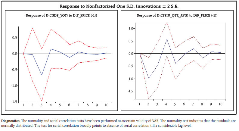
Annex C Assessment of Outlook on Prices on Consumer food price Objective: To assess the impact of outlook on prices on consumer food price inflation. Methodology: The simple VAR has been applied. Consumer food price inflation (Urban) has been selected instead of CPI(U) as food prices are perceived to be major driver of consumer opinion. Other variables viz., price outlook of consumers (F_PRICE) and GDP growth rate (CGDP_YOY) remain the same. Results: The VAR estimation results are reproduced below. It is noted that NR on price outlook has a negative and statistically significant influence on CFPI(U) inflation. The result is similar to as obtained for CPI(U) earlier. The impulse response function output shows decline in CFPI(U) inflation in the second and third quarters for a unit positive shock in households’ price outlook. | Vector Autoregression Estimates | | | D(F_PRICE(-1)) | D(CGDP_YOY) | D(CFPIU_QTR_AVG) | | D(F_PRICE(-2)) | -0.358258 | -0.004421 | -0.160053 | | | (0.21222) | (0.06747) | (0.06219) | | | [-1.68815] | [-0.06553] | [-2.57342] | | D(F_PRICE(-3)) | -0.167571 | -0.083494 | -0.180405 | | | (0.17877) | (0.05683) | (0.05239) | | | [-0.93735] | [-1.46910] | [-3.44336] | | D(CGDP_YOY(-1)) | -0.563549 | -0.348940 | -0.147654 | | | (0.61401) | (0.19520) | (0.17995) | | | [-0.91781] | [-1.78757] | [-0.82054] | | D(CGDP_YOY(-2)) | -0.209170 | -0.304952 | -0.249959 | | | (0.63758) | (0.20269) | (0.18685) | | | [-0.32807] | [-1.50450] | [-1.33773] | | D(CFPIU_QTR_AVG(-1)) | -1.515160 | 0.171402 | -0.304225 | | | (0.59238) | (0.18833) | (0.17361) | | | [-2.55774] | [ 0.91014] | [-1.75237] | | D(CFPIU_QTR_AVG(-2)) | -0.268130 | 0.194583 | -0.129990 | | | (0.67198) | (0.21363) | (0.19693) | | | [-0.39902] | [ 0.91084] | [-0.66007] | | C | -0.155411 | -0.238638 | -0.429229 | | | (1.16018) | (0.36884) | (0.34001) | | | [-0.13395] | [-0.64700] | [-1.26240] | | Log likelihood | | -207.5551 | | | Akaike information criterion | | 15.23701 | | | Schwarz criterion | | 16.21785 | |
| VAR Residual Normality Tests Null Hypothesis: residuals are multivariate normal | | Component | Skewness | Chi-sq | df | Prob. | | 1 | -0.114410 | 0.065448 | 1 | 0.7981 | | 2 | -0.459247 | 1.054537 | 1 | 0.3045 | | 3 | -0.590983 | 1.746303 | 1 | 0.1863 | | Joint | | 2.866288 | 3 | 0.4127 | | Component | Kurtosis | Chi-sq | df | Prob. | | 1 | 3.123091 | 0.018939 | 1 | 0.8905 | | 2 | 2.641624 | 0.160542 | 1 | 0.6887 | | 3 | 4.594247 | 3.177031 | 1 | 0.0747 | | Joint | | 3.356511 | 3 | 0.3399 | | Component | Jarque-Bera | df | Prob. | | | 1 | 0.084388 | 2 | 0.9587 | | | 2 | 1.215078 | 2 | 0.5447 | | | 3 | 4.923334 | 2 | 0.0853 | | | Joint | 6.222800 | 6 | 0.3987 | |
| VAR Residual Serial Correlation LM Tests Null Hypothesis: no serial correlation at lag order h | | Lags | LM-Stat | Prob | | 1 | 3.252131 | 0.9535 | | 2 | 7.317485 | 0.6041 | | 3 | 9.792047 | 0.3676 | | 4 | 5.926342 | 0.7473 | | 5 | 16.66884 | 0.0542 | | 6 | 5.029615 | 0.8317 | | 7 | 5.351994 | 0.8026 | | 8 | 15.27051 | 0.0838 | | 9 | 3.621473 | 0.9345 | | 10 | 2.451907 | 0.9821 | | 11 | 5.759237 | 0.7638 | | 12 | 6.085299 | 0.7314 | | Probs from chi-square with 9 df. | | Conclusion: The consumers’ outlook on price has a statistically significant impact on consumer food price inflation that is in tandem as noted for consumer price inflation. |
Annex D Analysis including dummy for implementation of ‘Inflation targeting’ Objective: To assess the impact of outlook on prices controlling for ‘inflation targeting’ on CPI(U) inflation. Methodology: The following simple linear regression is run. Y represents CPI(U) inflation. D is a dummy variable that captures inflation targeting period. D takes value unity from March 201514 onwards and zero otherwise. X1 stands for future NR on price. X2 represents GDP growth rate (current). All variables are first differenced to make them stationary before running OLS. | Results: | | Dependent Variable: D(CPIU_QTR_AVG) | | Variable | Coefficient | Std. Error | t-Statistic | Prob. | | C | -0.356478 | 0.254213 | -1.402282 | 0.1718 | | DUM1 | 0.294839 | 0.354665 | 0.831317 | 0.4128 | | DUM1*D(F_PRICE) | -0.062603 | 0.031304 | -1.999852 | 0.0553 | | D(CPIU_QTR_AVG(-1)) | -0.004275 | 0.168584 | -0.025356 | 0.9800 | | D(CGDP_YOY(-1)) | 0.019908 | 0.097676 | 0.203819 | 0.8400 |
| R-squared | 0.147673 | Mean dependent var | -0.210685 | | Adjusted R-squared | 0.025912 | S.D. dependent var | 1.020144 | | S.E. of regression | 1.006840 | Akaike info criterion | 2.990238 | | Sum squared resid | 28.38436 | Schwarz criterion | 3.216982 | | Log likelihood | -44.33893 | Hannan-Quinn criter. | 3.066530 | | F-statistic | 1.212808 | Durbin-Watson stat | 2.037184 | | Prob(F-statistic) | 0.327538 | | | The result shows consumers’ outlook on price to be having negative impact on CPI(U) inflation since March 2015 onwards. It essentially implies improvement of consumer expectations about price leads to decline in inflation since the implementation of inflation targeting regime of Reserve Bank. Diagnostics: Certain post estimation diagnostics are provided here. The Jarque-Bera test indicates normality of residuals. Moreover, test for serial correlation is also satisfactory. Breusch-Godfrey Serial Correlation LM Test:
Null hypothesis: No serial correlation at up to 2 lags | | F-statistic | 0.121139 | Prob. F(2,26) | 0.8864 | | Obs*R-squared | 0.304667 | Prob. Chi-Square(2) | 0.8587 | Conclusion: The result indicates improvement of consumer expectations about price leads to decline in inflation since the implementation of inflation targeting regime of Reserve Bank.
|