| Economic activity moderated during the financial year (FY) 2018-19 dragged down by subdued global demand and also some slack in government consumption expenditure. Inflation eased further to 3.4 per cent and undershot the target of 4 per cent for the second successive year, led by a sharp decline in food inflation. Monetary indicators such as currency, deposits and credit moved further towards their pre-demonetisation trend, reflecting underlying macroeconomic and financial developments. Financial markets exhibited resilience except sporadic volatility as evident from the buoyant equity market, two-way movement in INR and call money rate remained aligned to the policy repo rate albeit with downward bias. Public finances recorded modest deviations from budgetary targets of gross fiscal deficit across the general government. On the external front, net capital flows remained moderate relative to current account deficit, which led to depletion of foreign exchange reserves during the year. II.1 THE REAL ECONOMY II.1.1 Over the year gone by i.e., April 2018 to March 2019, macroeconomic and financial conditions underwent pronounced shifts that were largely unanticipated. Global growth, which had accelerated in a broad cyclical upswing through calendar year 2017 right up to the early part of 2018, began to shed momentum thereafter. By the second half of 2018, the weakening of the global expansion had spread across geographies, encircling advanced economies (AEs) and emerging market economies (EMEs) alike in its embrace. II.1.2 Several forces were at work, often in conjunction – the normalisation of monetary policy in the United States (US); escalation of trade tensions; volatile crude prices; uncertainty looming over Brexit; disruption in the auto sector in Germany due to stricter emission norms; the slowing down of the Chinese economy; macroeconomic crisis in some large EMEs; and the tightening of financial conditions. This cocktail of global spillovers stirred up turbulence in financial markets as risk on sentiment herded investors to safe havens, shunning EMEs as an asset class. In the event, these economies were confronted with capital outflows, currency depreciations and asset price volatility to which India too was not immune. In the second half of 2018-19 and especially in the early months of 2019, some global risks ebbed, with greater accommodation in monetary policies across the world, the easing of macroeconomic stress in the crisis-affected EMEs and some rekindling of investors’ risk appetite. Yet risks to global growth and its near-term outlook remain tilted to the downside. II.1.3 In this environment, real GDP growth in India which had weakened in 2017-18 after peaking in the year before, slid down to a five-year low in 2018-19 (Appendix Table 1). The loss of speed became evident from Q2 as some drivers of growth – notably investment – began to fade, albeit cushioned by still resilient consumption spending, both private and government. Through the second half of the year, high frequency indicators have flashed slowing sales growth among manufacturing and non-IT services sector corporations, with evidence of private consumption losing pace, especially in the fast-moving consumer goods (FMCG) segment. Financial conditions eased, but bank credit is yet to become broad-based and flow of resources from non-bank financial intermediaries has not yet gained its earlier traction. Abstracting from a brief surge in March 2019, export growth has decelerated and non-oil non-gold imports are in contraction mode, indicative of the underlying weakness of domestic demand. On the supply side, activity in manufacturing and in some categories of services, such as trade, transportation, communication and broadcasting moderated in the second half of the year and agricultural production remained modest, but in relation to the record levels achieved in the preceding two years. II.1.4 Overall the outlook appears clouded as the Indian economy begins its course through 2019-20. Against this backdrop, component-wise analysis of aggregate demand follows this Sub-section. Developments in aggregate supply conditions in terms of the performance of agriculture, value added in the industrial sector, and the resilient performance of services is sketched out in Sub-section 3, i.e., aggregate supply. An analysis of job creation in the economy based on high frequency indicators as also major policy initiatives in the area are covered in the last Sub-section. 2. Aggregate Demand II.1.5 The May 2019 release of the National Statistical Office (NSO) confirmed that aggregate demand, measured by year-on-year (y-o-y) growth of GDP at 6.8 per cent in 2018-19, weakened 0.4 percentage points in relation to the preceding year, and 0.3 percentage points below its decennial trend rate of 7.1 per cent. In fact, the GDP growth of 6.2 per cent in H2:2018-19 was the lowest in five years (Chart II.1.1). The slackening of demand in the economy was also evident in the opening of the negative output gap (i.e., deviation of actual output from its potential level) in Q3 and Q4 of 2018-19. 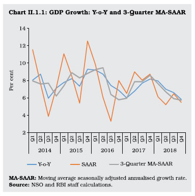 II.1.6 Over the period 2003-19, the performance of the economy reveals several interesting attributes (Table II.1.1). First, average GDP growth during 2014-19 has been robust by historical standards, but lower than the high growth phases of 2003-08 and 2009-11. Second, the expansion of aggregate demand in the 2014-19 phase was driven by robust consumption – both private and government – and could have buffered the economy from the transient shock of demonetisation. By contrast, burgeoning fixed investment was the driver of growth during 2003-08, and fiscal stimulus was the locomotive during 2009-11. As the stimulus wore off, growth slowed down in the next three years. | Table II.1.1: Underlying Drivers of Growth | | Components | Growth (per cent) | Contribution to Growth (per cent) | | 2003-08 | 2008-09 | 2009-11 | 2011-14 | 2014-19 | 2003-08 | 2008-09 | 2009-11 | 2011-14 | 2014-19 | | 1 | 2 | 3 | 4 | 5 | 6 | 7 | 8 | 9 | 10 | 11 | | I. Total Consumption Expenditure | 6.1 | 5.5 | 6.5 | 6.1 | 7.8 | 53.7 | 118.2 | 53.5 | 71.5 | 69.8 | | Private | 6.2 | 4.5 | 5.9 | 6.7 | 7.6 | 46.3 | 81.9 | 40.4 | 66.2 | 57.5 | | Government | 5.8 | 11.4 | 9.7 | 2.6 | 9.0 | 7.4 | 36.3 | 13.1 | 5.3 | 12.3 | | II. Gross Capital Formation | 15.3 | -2.6 | 14.5 | 2.0 | 7.1 | 58.5 | -31.4 | 64.1 | 16.6 | 32.9 | | Fixed investment | 12.6 | 3.2 | 9.4 | 6.2 | 7.4 | 43.1 | 32.6 | 35.9 | 37.9 | 31.7 | | Change in stocks | 73.5 | -51.4 | 56.2 | -27.4 | 15.3 | 12.5 | -75.4 | 17.9 | -16.7 | 0.7 | | Valuables | 27.8 | 26.9 | 45.0 | -11.1 | 4.9 | 3.0 | 11.4 | 10.3 | -4.6 | 0.6 | | III. Net Exports | | | | | | -7.7 | -72.4 | -4.1 | 8.9 | -10.5 | | Exports | 17.8 | 14.8 | 7.3 | 10.0 | 3.7 | 36.1 | 99.0 | 16.2 | 42.3 | 10.9 | | Imports | 20.0 | 22.4 | 6.9 | 6.1 | 6.5 | 43.8 | 171.4 | 20.3 | 33.4 | 21.4 | | IV. GDP | 7.9 | 3.1 | 8.2 | 5.7 | 7.5 | 100.0 | 100.0 | 100.0 | 100.0 | 100.0 | | Source: NSO and RBI staff calculations. | II.1.7 Compositional shifts in aggregate demand were evident during the year in terms of shares as well as weighted contributions (Chart II.1.2 and Appendix Table 2). Private final consumption expenditure (PFCE), the dominant component at 56.9 per cent of GDP, recorded a marginal increase in its share in 2018-19 in relation to a year ago, but its contribution to GDP growth in 2014-19 fell by 8.7 percentage points below its level in the preceding triennium, i.e., 2011-14. The resulting slack was partly filled by government final consumption expenditure (GFCE) – its contribution to GDP growth rose by 7 percentage points in 2014-19 vis-à-vis 2011-14. Even though gross fixed capital formation (GFCF) – the main constituent of investment in the economy – recorded an increase for the fifth successive year in 2018-19, its contribution to growth fell by 6.2 percentage points in 2014-19 in comparison with the preceding triennium. Notably, the drag from net exports came down significantly in 2018-19 on a year-on-year basis but their contribution to aggregate demand contracted sizeably in 2014-19 as against a positive contribution of 8.9 per cent in 2011-14. The evolution of net exports is covered in detail in Section II.6 on external sector. 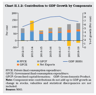 Consumption II.1.8 Consumption expenditure moderated during 2018-19. Nonetheless, its contribution to GDP increased for the second successive year. Private final consumption expenditure, the major component of aggregate demand, accelerated in the first half of the year, supported by higher disposable income on account of lower food expenses. The pick-up in activity in labour intensive sectors like construction provided additional cushion to household consumption demand. Rural demand, however, was affected by moderation in agricultural growth as reflected in tractors and two wheelers sales. Indicators of urban demand revealed a mixed picture in contrast. Air passenger traffic recorded its lowest growth in the last five years. Passenger vehicles sales were the lowest in five years on account of increase in insurance costs, volatile fuel prices, and lack of financing options due to the liquidity stress in the non-banking sector. The production of consumer non-durables slumped to its lowest level in the past three years. Going forward, public expenditure directed to rural areas through the Pradhan Mantri Kisan Samman Nidhi (PM-KISAN) and farm loan waivers by some states are expected to hold up rural demand. The analysis of high frequency information in the form of coincident economic indicators in the absence of concurrent GDP data helps in early assessment of economic activity as an input for policy formulation (Box II.1.1). Box II.1.1
Nowcasting India’s GDP Growth Globally, central banks rely on high-frequency economic indicators for a forward-looking assessment of the state of the economy, given the lags in the availability of official statistics. A Coincident Economic Indicator for India (CEII) is constructed using the single-index dynamic factor model (Stock and Watson, 1989) based on economic indicators which correlate strongly with the dynamics of GDP growth. Two indices are considered – a 6-indicator CEII comprising the production of consumer goods, non-oil non-gold imports, auto sales, rail freight, air cargo, and government receipts, and a 9-indicator CEII, which additionally includes IIP-core, exports, and foreign tourist inflows (Chart 1). A parsimonious autoregressive model of GDP growth augmented by CEII is used to nowcast quarterly GDP growth for the full period 2004:Q1-2019:Q1 (Table 1). The CEII emerges as statistically significant in explaining GDP growth, with the in-sample fit (adjusted R-squared) slightly higher for the 9-indicator model. However, the out-of-sample root mean squared error (RMSE) for the sample 2017:Q1-2019:Q1 is lower for the 6-indicator model. The nowcasts based on the 6-indicator and 9-indicator models along with the actual GDP growth are plotted in Chart 2A and 2B. It is observed that the nowcasts track GDP dynamics and turning points reasonably well over the estimation sample. In India, the first release of quarterly GDP is published approximately 7-8 weeks after the end of the reference quarter. To provide an early estimate, CEII is used to nowcast the current quarter GDP. Overall, the above findings indicate that the CEII based nowcasts help gauge the current state of the economy, thereby lending a greater degree of foresight to policy formulation. | Table 1: Nowcasting GDP Growth Using Coincident Economic Indicator for India | | Dependent Variable | GDP (Y-o-Y) | | Model 1 (6-Indicator) | Model 2 (9-Indicator) | | Constant | 3.05 | 2.81 | | CEII (Y-o-Y) | 2.91 | 3.96 | | GDP (Y-o-Y), Lag 1 | 0.38 | 0.32 | | Model Diagnostics | | | | Adjusted R-squared | 0.53 | 0.54 | | B-G Serial Correlation LM Test | 0.18 | 0.12 | | Out-of-Sample RMSE | 0.61 | 0.65 | Notes: 1. All coefficient estimates are significant at 1 per cent.
2. B-G test is for serial correlation in errors up to 12 lags.
3. Out-of-Sample RMSE pertains to 2017:Q1 to 2019:Q1. |
References: 1. Stock, J. H. and M. W. Watson (1989), ‘New Indexes of Coincident and Leading Economic Indicators’, NBER Macroeconomics Annual 1989, Vol. 4. 2. Gerlach, S. and M. S. Yiu (2004), ‘A Dynamic Factor Model for Current-Quarter Estimates of Economic Activity in Hong Kong’, Hong Kong Institute for Monetary Research, Working Paper No. 16. | Investment and Saving II.1.9 The rate of gross domestic investment in the Indian economy, measured by the ratio of gross capital formation (GCF) to GDP at current prices had risen to a peak of 39.8 per cent in 2010-11 before a prolonged slowdown set in taking it down to 30.9 per cent in 2016-17. A modest recovery took hold in the following year. Although data on gross domestic investment are not yet available for 2018-19, movement in its constituents suggest that the uptick could not be sustained. While the ratio of real gross fixed capital formation (GFCF) to GDP increased to 32.3 per cent in 2018-19 from 31.4 per cent in 2017-18, this upswing that started in Q3:2017-18 may have been a bounce-back from the transient impact of demonetisation and uncertainties related to the implementation of the GST that lasted for five consecutive quarters. However, growth in fixed investment collapsed to a fourteen-quarter low in Q4:2018-19 as production of capital goods registered a sharp contraction and imports nosedived in a coincident manner (Box II.1.2). Box II.1.2
Policy Uncertainty Index for India – Big Data Analysis Uncertainty prompts consumers and producers to alter their behaviour in terms of spending, investing and hiring decisions. Unanticipated outcomes on GDP growth, employment, stock indices and corporate earnings and even statements, actions and decisions made by policymakers with respect to fiscal, monetary, structural and regulatory policies, can turn out to be sources of uncertainty for economic agents and the wider macroeconomic environment. As a result, uncertainty has emerged as a key input into the decision making framework of policymakers across the globe. Unlike risk, which has a well-defined distribution of expected probabilities, uncertainty is unobservable. In the post-global financial crisis (GFC) period, however, the effects of uncertainty on macroeconomic and financial conditions appears to have become more pronounced and pervasive – uncertainty shocks have translated into investment slowdowns, and declines in economic activity and asset prices. These developments have imparted urgency to empirically capture and quantify the impact of uncertainty on the economy. These efforts can be broadly classified (a) volatility-based measures (Bloom, 2007); (b) dispersion in forecasts (Bachman, et al. 2013); (c) sentiment-based analysis using newspaper coverage frequency (Baker, et al. 2016); and (d) internet-based search intensity exercises (Castelnuovo and Tran 2017). An index, following Baker, et al. 2016, is constructed by text mining of leading Indian business news dailies1 to pick up the frequency of usage of keywords pertaining to ‘economic’ (E), ‘policy’ (P) and ‘uncertainty’ (U) or EPU (a news article must contain at least one word each belonging to EPU in order to be classified as signaling uncertainty), and a Google Uncertainty Index (GUI) following Castelnuovo and Tran 2017, based on internet search intensity of 70 keywords pertaining to fiscal, monetary and trade policies via Google Trends for the period January 2004 to June 2019. These indices reveal reasonably close co-movement with key macroeconomic variables, especially those related to production and investment. The indices are able to capture major domestic and external events that were expected to have contributed to uncertainty in the economy (Chart 1). They also exhibit strong correlations with conventional market-based volatility and risk indicators (Chart 2), such as India VIX Index and risk premia (calculated as the spread between 5-year AAA-rated corporate bonds and 5-year G-sec yields). A vector autoregression (VAR) model with four variables, i.e., GUI, the risk premia, real weighted-average lending rate and gross fixed capital formation (GFCF) to GDP ratio for the period 2005:Q1 to 2018:Q4, is estimated to analyse the impact of uncertainty on economic activity in India. The results of the VAR model suggest that there is an instantaneous increase in risk premia following an uncertainty shock (Chart 3). On the other hand, a three-quarter lagged negative impact is observed in respect of GFCF. The impulse response of GFCF to lending rates turn statistically significant from the fourth quarter onwards implying the impact of monetary policy on investments in a delayed manner, working mainly through the interest rate channel. Overall results suggest that uncertainty negatively impacts investment activity in India. References: 1. Bachmann, R., S. Elstner, and E. R. Sims (2013), ‘Uncertainty and Economic Activity: Evidence from Business Survey Data’, American Economic Journal: Macroeconomics, 5(2), 217-49. 2. Bloom, N. (2007), ’Uncertainty and the Dynamics of R&D’, American Economic Review, 97(2), 250-255. 3. Baker, S. R., N. Bloom, and S. J. Davis (2016), ’Measuring Economic Policy Uncertainty’ The Quarterly Journal of Economics, 131(4), 1593-1636. 4. Castelnuovo, E., and T. D. Tran (2017), ‘Google it Up! A Google Trends-based Uncertainty Index for the United States and Australia’, Economics Letters, 161, 149-153. | II.1.10 Among the determinants of GFCF, construction activity remained ebullient in 2018-19, driven by the government’s focus on infrastructure and affordable housing, and registered its highest growth in the last seven years. This was also reflected in its proximate coincident indicators – steel consumption and cement production (Chart II.1.3). For the year as a whole, growth in cement production at 13.3 per cent was the highest in the past ten years. Steel consumption continued to grow at a robust pace of 7.6 per cent despite a slowdown in automobile production. However, private investment in machinery and equipment exhibited signs of weakness with both its proximate coincident indicators – imports and production of capital goods – registering deceleration. II.1.11 At a disaggregated level, fixed investment in dwellings, other buildings and structures had declined by 0.3 percentage points to 15.4 per cent of GDP in 2017-18, mainly due to the household sector (Chart II.1.4). On the other hand, fixed investment in machinery and equipment led by the non-financial corporations and the household sector had increased to 12.0 per cent of GDP in 2017-18 from 11.3 per cent in 2016-17. Investment in intellectual property products (IPP) – expenditure on research and development; mineral exploration; computer software; and other intellectual property products by non-financial corporations – both public and private, had also picked up in 2017-18. Limited information that has become available for 2018-19 suggests that investment in dwellings, other buildings and structures, and IPP may register an increase while investment in machinery and equipment may exhibit a fall. 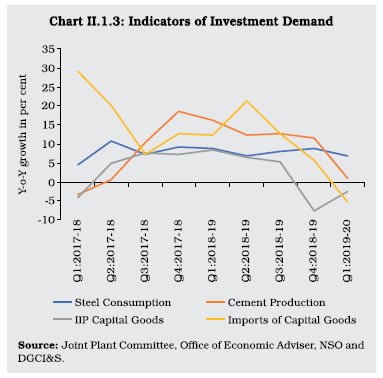 II.1.12 As per the Order Books, Inventories and Capacity Utilisation Survey (OBICUS) of the Reserve Bank, capacity utilisation in manufacturing rose through 2018-19, peaking at 76.1 per cent in Q4:2018-19. However, seasonally adjusted capacity utilisation declined by over one percentage point in Q4:2018-19. Declining sales led to an increase in inventory to sales ratio. The Industrial Outlook Survey (IOS) points to a modest improvement in demand conditions in Q2:2019-20 than in preceding quarters based on sentiments expressed on various parameters such as production, employment, exports and imports, capacity utilisation, and inventory position. However, with moderation expected in the cost of raw materials and optimistic outlook on overall financial situation, manufacturers are upbeat about profit margins in Q2:2019-20, despite pessimism in selling prices. 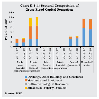 II.1.13 The rate of gross domestic saving had increased marginally to 30.1 per cent of gross national disposable income (GNDI) in 2017-18 from declines in the previous two years (Appendix Table 3A). While the saving of private non-financial corporations had increased marginally, the general government’s dissaving had increased. The household financial saving – the most important source of funds – had increased by 0.3 percentage points of GNDI, though it had remained much lower than 7.3 per cent during 2011-16 (Appendix Table 3B). II.1.14 The saving-investment gap has come down over the years, indicating that a larger part of the requirement to fund investment is being met through domestic resources and conversely, the net inflow of resources from abroad has declined, which corresponds to the degree of openness of the economy. The household sector continues to remain the net supplier of funds to the deficit sectors, i.e., non-financial corporations and general government (Chart II.1.5). In recent years, however, it is evident that resource gap of non-financial corporations, both public and private, has got significantly reduced, indicating that their investment needs are met through their internal resources. The drawdown on saving by the general government sector continues to remain at an elevated level. Developments in GFCE are addressed in Section II.5 on government finances. 3. Aggregate Supply II.1.15 Aggregate supply, measured by gross value added (GVA) at basic prices, slowed to 6.6 per cent in 2018-19, 30 basis points (bps) lower from a year ago and 20 bps lower than its decennial rate of 6.8 per cent (Appendix Table 2). Disentangling momentum from base effects, GVA’s quarter-on-quarter (q-o-q) seasonally adjusted annualised growth rate (SAAR) exhibited a turning point in Q4:2017-18 and weakened thereafter, barring a transient improvement in Q3:2018-19, notwithstanding favourable base effects in H1:2018-19 (Chart II.1.6), and underlying loss of speed appears to be a slowing down of productivity (Box II.1.3). II.1.16 An analysis of the growth path of the economy over the last 16 years from the supply side reveals that growth is primarily driven by services sector which has exhibited resilience over the entire period, barring 2008-09 (Table II.1.2). Secondly, growth of agriculture, forestry and fishing is unpredictable reflecting reliance on monsoon, though the increasing share of allied activities which is relatively insulated from weather uncertainties has imparted some resilience to the sector. Consequently, agriculture has lost its share in overall GVA to services sector. Industrial GVA on the other hand, has been driven by its largest constituent – manufacturing – and has broadly sustained its share, reflecting its forward and backward linkages with other sectors. 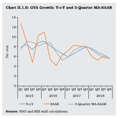
Box II.1.3
Drivers of Factor Productivity in India The global economy experienced a productivity slowdown since the global financial crisis (GFC) of 2008, with notable declines in both output per worker (labour productivity) and total factor productivity or TFP (Adler, et al., 2017). In India too, TFP growth decelerated from 1.8 per cent during 2003-07 to 0.8 per cent during 2008-16 (Chart 1). Improvement in labour productivity is attributed to (a) capital deepening; (b) efficiency in the existing capital stock; (c) quality of labour supply; and (d) TFP. In a growth accounting framework, TFP is captured as a residual (ECB, 2007 and Jorgenson et al., 2007), after adjusting for growth in labour and capital inputs. Over the period of study, a compositional shift is evident in sync with the GDP growth trajectory: the contribution of agriculture to TFP growth has fallen while that of services has gone up and manufacturing’s share has remained stable. Growth in value added in the agricultural sector has closely co-moved with its TFP growth, reflecting the lower importance of factor inputs in shaping agricultural performance (Chart 2). On the other hand, divergence has become marked in respect of both manufacturing and services, with TFP growth slowing down persistently in both sectors and markedly so in case of the latter, compared to value added (Chart 3). The contribution of TFP to services sector2 growth has been lower than for manufacturing, especially in recent years (Chart 4). Using a Harberger Plot3, it is observed that there are some consistent contributors to TFP growth like chemical and chemical products, post and telecommunications, and transport and storage (Chart 5). The penetration of information and communication technologies (ICT) has greatly benefited sectors like telecommunications, financial services and business services, and their importance in TFP growth has increased in recent years. Some sectors have, however, remained laggards over the years. In order to check for convergence across sectors, a panel regression is estimated in the form given below (European Commission, 2014).
In this specification, TFPgap captures convergence between leading sector and other industries while TFPmax captures spillover effects from the leading sector. A negative sign of TFPgap implies a larger potential gain for laggard industries with higher distance from the TFP frontier by adopting enhanced technology and advanced managerial practices. On the other hand, a positive sign of TFPmax suggests the existence of spillover of TFP from leading sector with high penetration of ICT like financial services to others. The regression results support presence of TFP convergence and spillover channels in India (Table 1). The fastest convergence is witnessed in the last period, i.e., 2009-16, when financial services emerged as the sector with the highest TFP. | Table 1: Sectoral Convergence and Spillover of TFP | | Variables | 1981-2016 | 1981-1992 | 1992-1999 | 2003-2007 | 2009-2016 | | 1 | 2 | 3 | 4 | 5 | 6 | | TFPgap | -0.047* | -0.269*** | -0.274* | -0.304* | -0.428*** | | | (0.023) | (0.063) | (0.136) | (0.174) | (0.107) | | TFPmax | 0.144** | 0.374*** | 1.054 | -1.396 | 2.762*** | | | (0.619) | (0.111) | (0.668) | (0.833) | (0.577) | | Constant | -0.065** | -0.393*** | -0.338** | -0.363* | -0.568*** | | | (0.282) | (0.091) | (0.151) | (0.199) | (0.136) | | Year fixed effects | Yes | Yes | Yes | Yes | Yes | | Observations | 972 | 324 | 216 | 135 | 216 | | R-squared | 0.08 | 0.24 | 0.12 | 0.13 | 0.29 | | Number of Indcode | 27 | 27 | 27 | 27 | 27 | | Robust standard errors in parentheses. *** p<0.01, ** p<0.05, * p<0.1 | Evidence from Harberger plot and convergence model suggests the need for higher investments in human capital through skilling and training to enable other sectors to adopt advanced technology and benefit through the convergence and spillover effects from industries using ICT technologies. References: 1. Adler, G., R. Duval, D. Furceri, S. K. Çelik, K. Koloskova, and M. Poplawski-Ribeiro (2017), ‘Gone with the Headwinds: Global Productivity’, IMF Staff Discussion Note, SDN/17/04. 2. ECB (2007), ‘Sectoral Patterns of Total Factor Productivity Growth in the Euro Area Countries’, European Central Bank Monthly Bulletin, pp. 57-61. 3. European Commission (2014), ‘The Drivers of Total Factor Productivity in Catching-up Economies’, Quarterly Report on the Euro Area, Vol.13(1), pp. 7-19. 4. Jorgenson, D. W., M. S. Ho, J. D. Samuels, and K. J. Stiroh (2007), ‘Industry Origins of the American Productivity Resurgence’, Economic Systems Research, 19(3), 229 –252. |
| Table II.1.2: Real GVA Growth | | Sectors | Growth (per cent) | Contribution to Growth (per cent) | | 2003-08 | 2008-09 | 2009-11 | 2011-14 | 2014-19 | 2003-08 | 2008-09 | 2009-11 | 2011-14 | 2014-19 | | 1 | 2 | 3 | 4 | 5 | 6 | 7 | 8 | 9 | 10 | 11 | | I. Agriculture, forestry and fishing | 4.5 | -0.2 | 4.0 | 4.5 | 2.9 | 12.0 | -1.2 | 8.7 | 14.6 | 6.1 | | II. Industry | 8.4 | 3.4 | 9.1 | 2.9 | 8.1 | 24.9 | 18.6 | 29.2 | 11.8 | 25.1 | | i. Mining and quarrying | 5.2 | -2.5 | 9.7 | -5.6 | 7.1 | 3.1 | -2.4 | 5.0 | -4.4 | 2.8 | | ii. Manufacturing | 9.6 | 4.7 | 9.3 | 4.5 | 8.4 | 19.7 | 18.5 | 22.2 | 14.1 | 20.0 | | ii. Electricity, gas, water supply and other utility services | 7.1 | 4.9 | 6.5 | 5.1 | 7.5 | 2.1 | 2.5 | 2.0 | 2.1 | 2.3 | | III. Services | 8.6 | 6.4 | 8.0 | 7.0 | 8.2 | 62.0 | 82.6 | 62.1 | 73.6 | 68.8 | | i. Construction | 12.8 | 5.6 | 6.4 | 5.4 | 5.7 | 13.4 | 11.6 | 7.9 | 9.0 | 6.5 | | ii. Trade, hotels, transport, communication and services related to broadcasting | 9.4 | 2.4 | 9.0 | 7.5 | 8.4 | 20.3 | 9.6 | 19.8 | 24.0 | 21.4 | | iii. Financial, real estate and professional services | 7.6 | 5.2 | 5.6 | 8.5 | 8.8 | 19.4 | 23.5 | 15.0 | 28.8 | 25.7 | | iv. Public administration, defence and other services | 6.3 | 15.8 | 11.8 | 5.1 | 8.8 | 8.9 | 37.8 | 19.4 | 11.7 | 15.2 | | IV. GVA at basic prices | 7.7 | 4.3 | 7.4 | 5.6 | 7.3 | 100.0 | 100.0 | 100.0 | 100.0 | 100.0 | | Source: NSO and RBI staff calculations. | II.1.17 GVA by agriculture and allied activities grew by 2.9 per cent in 2018-19; while the increase in foodgrains and horticulture production turned out to be modest after two successive years of record production, final estimates may reveal a new record, going by the catch-up underway in moving from first to fourth advance estimates. The contribution of agriculture and allied activities to overall GVA growth declined to 6.6 per cent in 2018-19 but remained higher than that of 6.1 per cent during 2014-19. II.1.18 The south-west monsoon 2018 started off well but lost momentum during mid-July to mid-September, with uneven distribution of rainfall across states (Chart II.1.7a). Overall, the cumulative rainfall during the south-west monsoon season was 9 per cent below the Long Period Average (LPA). This took its toll on kharif sowing, initially exacerbated by delayed announcement of minimum support prices (MSPs), and persisting deflation in wholesale prices of kharif crops, but there was a catch up in the closing weeks of the season. As per the fourth advance estimates of the Ministry of Agriculture and Farmers’ Welfare, kharif foodgrains production increased by 0.9 per cent in 2018-19 over the final estimates for 2017-18. The production of rice increased by 5.1 per cent, buoyed by a 12.9 per cent hike in MSP for paddy. Output of pulses and coarse cereals, however, declined. Among the cash crops, growth in production of sugarcane at 5.3 per cent was higher than 2.8 per cent average growth of last five years, but cotton output fell by 12.5 per cent as compared to the previous year due to deficient rainfall in major growing states of Gujarat, Maharashtra, Telangana and Karnataka.  II.1.19 Rabi sowing was delayed due to late harvesting of the kharif crops and it could not catch up with the previous year’s level. In addition, it was hobbled by a deficiency in the north-east monsoon rainfall (44 per cent below the LPA) (Chart II.1.7b) and rabi foodgrains production declined by 0.9 per cent in 2018-19 over the final estimates for 2017-18. Wheat weathered the broad-based decline, however, exceeding the previous year’s bumper production (Table II.1.3). Overall, the foodgrains production in 2018-19 is estimated at 285 million tonnes – same as the record level achieved in 2017-18. While the production of rice and wheat set a record, the output of pulses and coarse cereals declined. | Table II.1.3: Agricultural Production 2018-19 | | (Million Tonnes) | | Crop | Season | 2017-18 | 2018-19 | 2018-19 Variation (Per cent) | | 4th AE | Final | Target | 3rd AE | 4th AE | Over 2017-18 | Over 2018-19 | | 4th AE | Final | 3rd AE | Target | | 1 | 2 | 3 | 4 | 5 | 6 | 7 | 8 | 9 | 10 | 11 | | Rice | Kharif | 97.5 | 97.1 | 99.0 | 101.7 | 102.1 | 4.7 | 5.1 | 0.4 | 3.2 | | | Rabi | 15.4 | 15.6 | 15.0 | 13.9 | 14.3 | -7.3 | -8.5 | 3.0 | -4.7 | | | Total | 112.9 | 112.8 | 114.0 | 115.6 | 116.4 | 3.1 | 3.2 | 0.7 | 2.1 | | Wheat | Rabi | 99.7 | 99.9 | 102.2 | 101.2 | 102.2 | 2.5 | 2.3 | 1.0 | 0.0 | | Coarse Cereals | Kharif | 33.9 | 34.0 | 35.7 | 32.5 | 31.0 | -8.6 | -8.9 | -4.6 | -13.2 | | | Rabi | 13.1 | 12.9 | 12.4 | 10.8 | 12.0 | -8.7 | -7.6 | 10.3 | -3.5 | | | Total | 47.0 | 47.0 | 48.1 | 43.3 | 43.0 | -8.6 | -8.6 | -0.9 | -10.7 | | Pulses | Kharif | 9.3 | 9.3 | 9.9 | 8.5 | 8.6 | -8.0 | -7.7 | 0.8 | -12.8 | | | Rabi | 15.9 | 16.1 | 16.1 | 14.7 | 14.8 | -6.9 | -8.1 | 0.7 | -8.1 | | | Total | 25.2 | 25.4 | 26.0 | 23.2 | 23.4 | -7.3 | -7.9 | 0.8 | -9.8 | | Foodgrains | Kharif | 140.7 | 140.5 | 144.6 | 142.8 | 141.7 | 0.7 | 0.9 | -0.7 | -2.0 | | | Rabi | 144.1 | 144.5 | 145.7 | 140.6 | 143.2 | -0.6 | -0.9 | 1.9 | -1.7 | | | Total | 284.8 | 285.0 | 290.3 | 283.4 | 285.0 | 0.0 | 0.0 | 0.6 | -1.8 | | Oilseeds | Kharif | 21.0 | 21.0 | 25.5 | 21.0 | 21.3 | 1.3 | 1.3 | 1.4 | -16.6 | | | Rabi | 10.3 | 10.5 | 10.5 | 10.4 | 11.0 | 6.5 | 5.0 | 5.3 | 4.6 | | | Total | 31.3 | 31.5 | 36.0 | 31.4 | 32.3 | 3.0 | 2.5 | 2.7 | -10.4 | | Sugarcane (Cane) | | 376.9 | 379.9 | 385.0 | 400.4 | 400.2 | 6.2 | 5.3 | -0.1 | 3.9 | | Cotton # | | 34.9 | 32.8 | 35.5 | 27.6 | 28.7 | -17.7 | -12.5 | 4.0 | -19.1 | | Jute & Mesta ## | | 10.1 | 10.0 | 11.2 | 9.8 | 9.8 | -3.6 | -2.6 | -0.3 | -12.8 | #: Lakh bales of 170 kgs. each. AE: Advance Estimates
# #: Lakh bales of 180 kgs. each.
Source: Ministry of Agriculture and Farmers Welfare, GoI. | II.1.20 The stock positions in respect of rice and wheat with the Food Corporation of India (FCI) during 2018-19 were on average higher by 2.9 times and 2.5 times, respectively, than the buffer norms. This has necessitated an increase in offtake through the open market sale of 4.12 per cent of annual production in 2018-19 compared to 0.87 per cent of production in the previous year. The surplus food stock and unusually depressed food prices contributed to agrarian distress, including rising indebtedness and sluggish rural wages which calls for proactive and effective supply management policies (Box II.1.4). Box II.1.4:
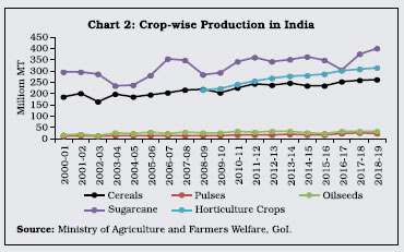
The Problems of Plenty Yield improvement and acreage expansion has boosted the production of cereals, oilseeds and sugar across the world. Wheat production increased significantly in the Black Sea region (Russian Federation, Ukraine and Kazakhstan), due to crop land expansion, crop intensification, investment in fertilisers, machinery and storage facilities by the big agricultural companies. Corn production received a boost in Alaska through area expansion, supported by innovations in hybrid seed technology (Reuters, 2017). As a result, world cereal production outstripped utilisation in most of the years during 2006-07 to 2018-19 (Chart 1a). Stockpiles of cereals, sugar and oilseeds are at all-time highs (Charts 1b, 1c, and 1d). In India, back-to-back years of bumper production of cereals, pulses, oilseeds and horticulture crops in 2016-17 and 2017-18 (Chart 2) has led to the build-up of comfortable stocks. Improvements in supply chains, access to low cost mobile phones, micro-finance and supply management, albeit reactive and inopportune, have all contributed to the rare emergence of excess supplies. 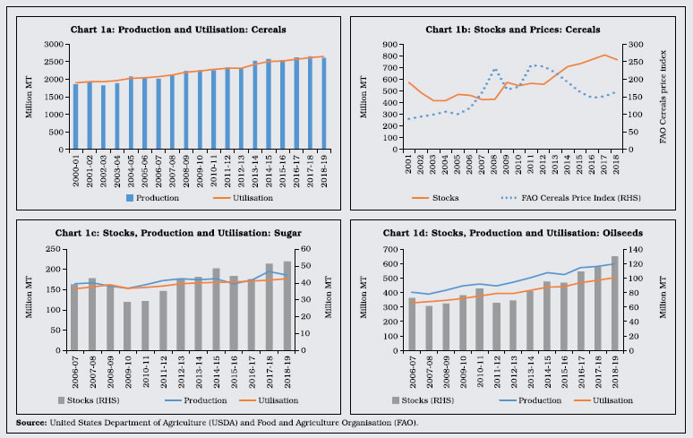
 Disentangling the various factors at work in a panel data model [pooling crop level data, Singh et al. (2014)] for the period from 2006-07 to 2018-19, it is observed that the effects of expanding area under cultivation and boosting yield on the value of output are positive and significant – the ‘area’ effect in the period 2016-17 to 2018-19 is lower than during 2006-07 to 2012-13, but the yield effect is higher4. The effect of relative prices is lower in the recent period because domestic prices were higher than international prices, leading to erosion in the competitiveness of India’s farm exports and increased imports, which augmented domestic supply and depressed domestic prices. References: 1. Reuters, (2017), ‘Drowning in Grain - Reuters Special Report on the Global Grains Glut’, Reuters, accessed at https://farmpolicynews.illinois.edu/2017/09/drowning-grain-reuters-special-report-global-grains-glut/ 2. Singh, B.P., P.K. Joshi, D.S. Negi and S. Agarwal (2014), ‘Changing Source of Growth in Indian Agriculture: Implications for Regional Priorities for Accelerating Agriculture Growth’, Working Paper 01325, IFPRI, Washington, USA. | Horticulture II.1.21 Horticulture, with a share of 33 per cent in agricultural GVA, has outpaced the production of foodgrains since 2012-13. As per the second advance estimates, the production of horticulture crops at 314.9 million tonnes in 2018-19 is a record, driven mainly by spices, flowers and vegetables (Table II.1.4). Policy Initiatives II.1.22 MSPs announced in kharif 2018-19, were ranging between 3.7-52.5 per cent above those announced in the previous year. The government announced ‘Pradhan Mantri Annadata Aay SanraksHan Abhiyan’ (PM-AASHA), an umbrella scheme to ensure reasonable prices for the crops including cereals, pulses, oilseeds, jute and cotton, for effective implementation of MSP. The MSP increase was lower as compared to last year for all the major rabi crops. | Table II.1.4: Horticulture Production | | (Million Tonnes) | | Crops | 2017-18 | 2018-19 | Variation (Per cent) | | 2nd AE | Final Estimate (FE) | 1st AE | 2nd AE | 2018-19 2nd AE over 2017-18 2nd AE | 2018-19 2nd AE over the 2017-18 FE | 2018-19 2nd AE over the 2018-19 1st AE | | 1 | 2 | 3 | 4 | 5 | 6 | 7 | 8 | | Total Fruits | 94.4 | 97.4 | 96.8 | 97.4 | 3.2 | 0.0 | 0.6 | | Banana | 29.3 | 30.8 | 30.0 | 31.2 | 6.6 | 1.3 | 4.0 | | Citrus | 12.5 | 12.5 | 12.3 | 13.2 | 5.1 | 4.8 | 7.3 | | Mango | 20.5 | 21.8 | 22.4 | 21.0 | 2.1 | -4.0 | -6.3 | | Total Vegetables | 182.0 | 184.4 | 187.5 | 187.4 | 2.9 | 1.6 | -0.1 | | Onion | 21.8 | 23.3 | 23.6 | 23.3 | 6.6 | 0.1 | -1.4 | | Potato | 50.3 | 51.3 | 52.6 | 53.0 | 5.2 | 3.2 | 0.7 | | Tomato | 22.1 | 19.8 | 20.5 | 19.7 | -10.9 | -0.5 | -4.1 | | Plantation Crops | 18.5 | 18.1 | 18.0 | 17.7 | -4.3 | -2.3 | -1.8 | | Total Spices | 8.5 | 8.1 | 8.6 | 8.6 | 0.8 | 6.0 | 0.3 | | Aromatics and Medicinal | 1.1 | 0.9 | 0.9 | 0.8 | -20.2 | -2.3 | -4.8 | | Total flowers | 2.6 | 2.8 | 2.9 | 2.9 | 12.1 | 3.9 | 1.2 | | Total | 307.2 | 311.7 | 314.7 | 314.9 | 2.5 | 1.0 | 0.1 | FE: Final Estimate AE: Advance Estimate
Source: Ministry of Agriculture and Farmers Welfare, GoI. | II.1.23 In order to increase milk production and overall development of the dairy sector, the government has set up a dairy processing and infrastructure development fund (DIDF). It has created a separate Department of Fisheries to provide sustained and focussed attention on the development of the sector. Besides, the government has also approved setting up of a dedicated Fisheries and Aquaculture Infrastructure Development Fund (FIDF) to fill the large infrastructure gaps in fisheries sector. It has also approved a scheme for controlling the foot and mouth disease of livestock. II.1.24 MSP announced for kharif 2019-20 has not changed significantly from the previous year. In continuation with the last year, MSPs have been fixed in such a way that it ensures a minimum return of 50 per cent over the cost of production. In order to provide income support to farmers, in the interim Union Budget 2019-20, the government announced the Pradhan Mantri Kisan Samman Nidhi (PM-KISAN), under which vulnerable farmers holding cultivable land up to 2 hectares will receive a direct income support of ₹6,000 per annum (in three instalments of ₹2,000 each) from the central government. Recently, the government has extended this scheme, benefitting around 14.5 crore farmers. Another recent initiative by the government is Pradhan Mantri Kisan Pension Yojana – under which small and marginal farmers of age between 18 to 40 years will get a minimum fixed pension of ₹3,000 per month on attaining the age of 60 years by contributing voluntarily, with government contributing an equal amount, to the pension fund. The scheme is expected to cover 5 crore small and marginal farmers in the first three years. The Union Budget 2019- 20 announced in July has recognised the need for forming new Farmer Producer Organisations (FPO), expansion of benefits of e-NAM (online agricultural trading platform) to larger number of farmers and introduction of Zero Budget Farming for increasing the farmers’ income. The Budget has also proposed to launch Pradhan Mantri Matsya Sampada Yojana (PMMSY) to establish a robust fisheries management framework. Further, the government has extended the benefit of interest subvention and the facility of prompt repayment incentive of 3 per cent for rescheduled loans to animal husbandry and fisheries. 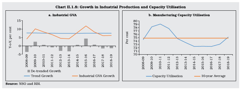 Industrial Sector II.1.25 GVA growth in industry accelerated marginally on a y-o-y basis to 6.2 per cent in 2018-19 breaking the sequence of two consecutive years of deceleration. Cyclical component of industrial GVA growth (estimated through a univariate approach using Hodrick- Prescott filter) remained negative during the year while the capacity utilisation in manufacturing recovered sharply over 10-year average level (Chart II.1.8 a & b). On the other hand, the index of industrial production (IIP) growth decelerated during 2018-19 to a 3-year low of 3.8 per cent driven by deceleration in manufacturing. Among the sectoral components of IIP, the growth in mining and electricity generation has been relatively stable during the year. During Q1:2019-20, a sharp upsurge in the electricity growth was recorded while manufacturing and mining remained stable (Chart II.1.9). 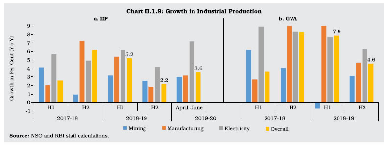 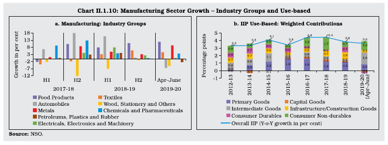 II.1.26 Manufacturing GVA growth reached a 9-quarter high of 12.1 per cent during Q1:2018-19 helped by a favourable base and gain in momentum, before slowing down from Q2:2018-19. Headwinds emanating from subdued demand – both domestic and international, and higher input costs especially oil based, led to slowdown in manufacturing and a widening wedge between IIP and GVA growth. II.1.27 The deceleration in manufacturing during H2:2018-19 – which constitutes three-fourth of industry was on account of the contraction/deceleration in six out of eight broad industry groups constituting 84.2 per cent of manufacturing IIP, i.e., automobiles; electrical, electronics and machinery; chemicals and pharmaceuticals; metals; petroleum, plastic and rubber; and wood, stationery and others. Only two broad industry groups, i.e., food products and textiles registered acceleration (Chart II.1.10a). In terms of use-based classification, much of the deceleration in manufacturing IIP can be traced to the deceleration in intermediate goods, capital goods and consumer non-durables (also reflected in sales of FMCG companies) (Table II.1.5). In terms of weighted contributions, the fall in consumer non-durables was the heaviest, followed by intermediate goods and capital goods, respectively. Capital goods production remained subdued while intermediate and consumer non-durables recovered sharply in Q1:2019-20 (Chart II.1.10b). II.1.28 The improvement in the mining sector was on account of sharp pick-up in coal production that more than compensated for the contraction in crude oil and deceleration in natural gas production. Even with a sharp acceleration in coal production, thermal electricity generation slowed down which was partly compensated by strong growth in hydro and renewable generation. Slowdown in manufacturing activities also contributed to reduced demand of electricity by the industrial sector. Historically, IIP manufacturing and electricity generation co-move closely, indicating that a pick-up in manufacturing activities is essential for electricity demand to improve. The power sector, especially, the thermal segment – the mainstay of power supply with around 76 per cent share – at the current juncture is faced with multiple challenges – cheaper and rising share of renewable energy in the overall energy mix (from 3.7 per cent in 2008-09 to 9.2 per cent during 2018-19); market based short-term price discovery through energy exchange at lower price than long-term forward power purchase agreements (PPAs)5 and DISCOMs reeling with financial stress. | Table II.1.5: Index of Industrial Production (Base 2011-12) | | (Per cent) | | Industry Group | Weight in IIP | Growth Rate | | 2014-15 | 2015-16 | 2016-17 | 2017-18 | 2018-19 | Apr-June 2018 | Apr-June 2019 | | 1 | 2 | 3 | 4 | 5 | 6 | 7 | 8 | 9 | | Overall IIP | 100.0 | 4.0 | 3.3 | 4.6 | 4.4 | 3.8 | 5.1 | 3.6 | | Mining | 14.4 | -1.4 | 4.3 | 5.3 | 2.3 | 2.9 | 5.4 | 3.0 | | Manufacturing | 77.6 | 3.8 | 2.8 | 4.4 | 4.6 | 3.9 | 5.1 | 3.2 | | Electricity | 8.0 | 14.8 | 5.7 | 5.8 | 5.4 | 5.2 | 4.9 | 7.2 | | Use-based | | | | | | | | | | Primary goods | 34.0 | 3.8 | 5.0 | 4.9 | 3.7 | 3.5 | 5.9 | 2.6 | | Capital goods | 8.2 | -1.1 | 3.0 | 3.2 | 4.0 | 2.7 | 8.6 | -2.2 | | Intermediate goods | 17.2 | 6.1 | 1.5 | 3.3 | 2.3 | 0.9 | 0.7 | 9.3 | | Infrastructure/Construction goods | 12.3 | 5.0 | 2.8 | 3.9 | 5.6 | 7.3 | 8.5 | 2.4 | | Consumer durables | 12.8 | 4.0 | 3.4 | 2.9 | 0.8 | 5.5 | 8.1 | -1.0 | | Consumer non-durables | 15.3 | 3.8 | 2.6 | 7.9 | 10.6 | 4.0 | 2.0 | 7.3 | | Source: NSO. | II.1.29 Indicators of financial performance of listed manufacturing firms also reveal that the sales growth and EBITDA margin peaked in Q1:2018-19 before declining in Q3-Q4:2018-19. As regards expectations, manufacturing firms polled in the Reserve Bank’s Industrial Outlook Survey turned optimistic in Q3-Q4:2018-19, but expectations dipped in Q1-Q2:2019-20 due to weaker prospects for production, order books, profit margins and overall financial situation. Services Sector II.1.30 In contrast to the industrial sector, the services sector growth decelerated on a y-o-y basis in 2018-19 extending a sequence beginning in 2015-16. Moreover, the cushion provided by public administration, defence and other services (PADO) waned. Excluding general government services embodied in PADO, services sector GVA accelerated from 6.7 per cent in 2017-18 to 7.4 per cent in 2018-19. Though some recovery was seen in the cyclical component of services GVA (excluding PADO) growth (estimated through a univariate approach using Hodrick- Prescott filter), it remained negative during the year (Chart II.1.11).
II.1.31 Among the components of services, GVA in the construction sector continued its trend of acceleration beginning 2012-13 (Chart II.1.12a), as reflected in strong growth in steel consumption and cement production during the year on the back of the support from government’s focus on infrastructure and affordable housing. II.1.32 In terms of weighted contributions to growth, financial, real estate and professional services showed improvement (Chart II.1.12b) with key indicators of financial services, i.e., aggregate deposits and bank credit growth picking up and EBITDA of IT services firms accelerating. Weighted contribution of trade, hotels, transport, communication and services related to broadcasting to services growth declined in 2018-19. Among the indicators of the road transport segment, sales of new commercial vehicles slowed down amid a broad-based deceleration in the automobile sector in H2:2018-19. The aviation sector also recorded deceleration from January 2019 primarily due to financial stress in one major airline reflected in domestic air passenger traffic, which had recorded a double-digit growth for 52 months in a row up to December 2018. Only rail transport witnessed marginal improvement in terms of growth of net tonne kilometres of freight. II.1.33 The Reserve Bank’s service sector composite index (SSCI), which combines information collated from high frequency indicators and leads GVA growth in the services sector, is indicating moderation in Q1:2019-20 (Chart II.1.13). 4. Employment II.1.34 The National Statistical Office (NSO) in May 2019 released the Periodic Labour Force Survey (PLFS) which indicates higher regularisation of work force in 2017-18 as compared to previous rounds of Employment and Unemployment Surveys (EUS). Among total workforce, the share of regular/salaried was higher at 45.7 per cent (43.4 per cent in 2011-12) and 52.1 per cent (42.8 per cent in 2011-12) for urban male and female, respectively. In rural areas also, the share of regular/salaried workforce increased in 2017-18, though their share was still low at 14 per cent for male (10.0 per cent in 2011-12) and 10.5 per cent for female (5.6 per cent in 2011-12). The usual status unemployment rate at 6.1 per cent (6.2 per cent for male and 5.7 per cent for female) in 2017-18, as per the PLFS, may not be strictly comparable with the previous rounds of EUS due to difference in methodology. 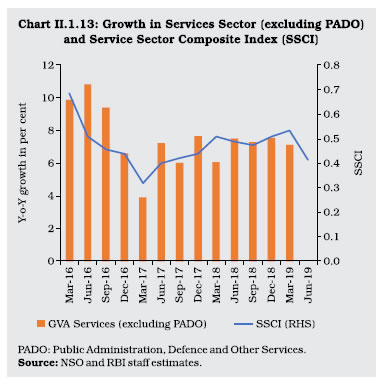 II.1.35 Information on formal sector employment, compiled from payroll6 data of Employees’ Provident Fund Organisation (EPFO), Employees’ State Insurance Corporation (ESIC) and National Pension System (NPS), indicates a mixed picture with regard to job creation in 2018-19 vis-à-vis 2017-187. Net new subscribers added to EPFO per month increased (0.56 million in 2018-19 from 0.19 million during 2017-18) while new subscribers to NPS slowed down. The number of members who paid their contributions to ESIC increased marginally during 2018-19. II.1.36 Several policy initiatives were taken by the government during the year to boost employment generation. Keeping in view the large employment potential in entertainment industry, single window clearance facility for ease of shooting films, currently available only to foreigners, will be made available to Indian filmmakers as well from 2019-20. The government has also undertaken several steps to strengthen the micro, small and medium enterprises (MSMEs) sector, which provides a lucrative avenue for employment. A scheme of sanctioning loans up to ₹10 million in 59 minutes was put in place for MSMEs. Further, over 10 million youth are being trained every year to help them earn a livelihood through Pradhan Mantri Kaushal Vikas Yojana. Employment for the youth is also being promoted through self-employment schemes including MUDRA, Start-up India and Stand-up India. II.1.37 To sum up, consumption demand remained resilient during 2018-19, albeit with some moderation vis-à-vis the previous year while gross fixed capital formation which sustained momentum in the first half of the year weakened thereafter in an environment of political uncertainty amidst general elections. External demand operated as a drag for the second successive year. Deficit south-west monsoon and depleted reservoirs dented the performance of agriculture sector. While the industrial sector posted resilient growth mainly driven by manufacturing in the first half, the momentum in construction and financial services sustained the healthy growth of overall services sector. The official estimates suggest more regularisation of employment in 2017-18 and various initiatives undertaken by the government are expected to create avenues for employment generation. Going forward, priority should be accorded to revive consumption and private investment while continuing with structural reforms. II.2 PRICE SITUATION II.2.1 Commodity price developments significantly shaped the global inflation environment during 2018 and the early months of 2019. Food prices, in particular, softened markedly in 2018, before a recovery took hold beginning 2019 on the back of firming prices of sugar, dairy products and animal proteins. Metal prices eased, especially from the second half of 2018, on weaker demand from China, although they turned up from February 2019, buoyed by improved global market sentiments and supply disruptions. Crude oil prices came off their October 2018 peak and fell by almost 30 per cent by December 2018, enabled by higher shale production in the US and weakening global demand. Production cuts by Organisation of the Petroleum Exporting Countries (OPEC) and other major producers along with supply disruptions in Venezuela firmed up crude prices in early 2019. II.2.2 In this milieu, retail inflation measured by consumer prices remained subdued across advanced and emerging market economies (EMEs). In the former, even core inflation remained below targets with wage growth sluggish and demand weakened by slowing global economic activity. In many EMEs, inflation pressures generally moderated, driven down by commodity prices and country-specific supply improvements, especially in respect of food items. II.2.3 In India, headline inflation8 eased significantly to average 3.4 per cent during 2018-19, the lowest annual reading in the new consumer price index (CPI) series (Table II.2.1). Accordingly, inflation has undershot the target of 4 per cent for the second financial year in succession under the remit of the monetary policy committee that was formally appointed in September 2016 under the new monetary policy framework. During Q1:2019-20, inflation has remained moderate, averaging at 3.1 per cent. II.2.4 A sharp decline in food inflation, and an elevated and sticky inflation excluding food and fuel were the defining features of price dynamics in 2018-19, with the persistent wedge between headline inflation and inflation excluding food and fuel becoming a subject of animated public debate (Chart II.2.1). Against this backdrop, Sub-section 2 assesses developments in global commodity prices and inflation. Sub-section 3 discusses movements in domestic headline inflation and major turning points. Sub-section 4 drills down into the granular aspects of price developments in respect of major components, viz., food, fuel, and inflation excluding food and fuel. Sub-section 5 discusses other indicators of prices and costs as well as movements in wages. | Table II.2.1: Headline Inflation – Key Summary Statistics | | (Per cent) | | Statistics | 2012-13 | 2013-14 | 2014-15 | 2015-16 | 2016-17 | 2017-18 | 2018-19 | | 1 | 2 | 3 | 4 | 5 | 6 | 7 | 8 | | Mean | 10.0 | 9.4 | 5.8 | 4.9 | 4.5 | 3.6 | 3.4 | | Standard deviation | 0.5 | 1.3 | 1.5 | 0.7 | 1.0 | 1.2 | 1.1 | | Skewness | 0.2 | -0.2 | -0.1 | -0.9 | 0.2 | -0.2 | 0.1 | | Kurtosis | -0.2 | -0.5 | -1.0 | -0.1 | -1.6 | -1.0 | -1.5 | | Median | 10.1 | 9.5 | 5.5 | 5.0 | 4.3 | 3.4 | 3.5 | | Maximum | 10.9 | 11.5 | 7.9 | 5.7 | 6.1 | 5.2 | 4.9 | | Minimum | 9.3 | 7.3 | 3.3 | 3.7 | 3.2 | 1.5 | 2.0 | Note: Skewness and kurtosis are unit-free.
Source: National Statistical Office (NSO), and RBI staff estimates. |
2. Global Inflation Developments II.2.5 International food prices, especially of sugar, dairy products and edible oils, remained generally soft during 2018, reflecting abundant supply (Chart II.2.2). In the non-food category, price pressures in metals remained largely weak due to US-China trade tensions and weak global demand. Global crude oil prices reached US$ 77 per barrel9 in October 2018 – the highest level since December 2014 – following the decision of the OPEC and non-OPEC producers, led by Russia, in November 2017 to extend cuts in oil production by 1.8 million barrels per day till the end of 2018, and US sanctions on exports from Iran. The price of the Indian basket of crude oil moved in tandem and rose to US$ 80 per barrel in October 2018. However, global crude oil prices softened sharply during November-December 2018 on concerns of oversupply amidst weakening of global growth and heightened trade tensions. Prices picked up again during January-March 2019 due to stricter compliance by OPEC members to voluntary reductions in production and increasing crude oil supply disruptions. The price of the Indian basket also increased to US$ 67 per barrel in March 2019 from US$ 58 per barrel in December 2018 in line with global prices. 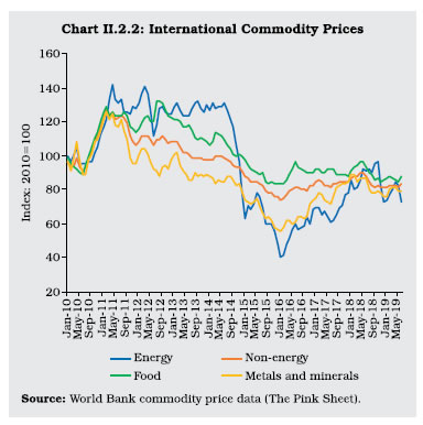 II.2.6 Reflecting generally soft global commodity price conditions, consumer price inflation remained benign during 2018 and 2019 so far in a number of economies, both advanced and emerging markets. Wage growth remained sluggish despite lower unemployment, effectively muting potential price-wage feedback loops. Accordingly, inflation expectations also remained contained. Many EMEs also experienced easing of inflation pressures, except in countries like Argentina and Turkey faced with country-specific idiosyncrasies. In the second half of 2018, a number of global macro-economic developments such as escalation of US-China trade tensions, regulatory tightening in China to rein in debt, and tightening of financial conditions in line with monetary policy normalisation in some major advanced economies adversely impacted growth and thereby added to the downward pressure on commodity prices and inflation. 3. Headline CPI Inflation in India II.2.7 Headline inflation in India eased during 2018-19 along with a marginal fall in its dispersion (Table II.2.1). The intra-year distribution of inflation was also more balanced relative to preceding year as reflected in the near zero positive skew. Furthermore, the higher negative kurtosis than a year ago suggests fewer instances of large deviations from mean inflation during the year, which is also reflected in the reduced gap between maximum and minimum inflation during the year. This change in the distribution of inflation was essentially brought about by movements in its constituents, mainly food, within a narrow range during the year. II.2.8 At a disaggregated level, price pressures in food, and excluding food and fuel groups drove up headline inflation to an intra-year peak of 4.9 per cent in June 2018. Food price inflation eased thereafter, aided by favourable base effects. Contrary to usual historical price movements, the momentum of food prices turned negative from September 2018, dragging food prices into deflation in October 2018. The onset of the usual winter easing in prices of vegetables and fruits accentuated the decline to (-) 1.7 per cent in November 2018, the lowest in the new CPI series, and extended the deflation till February 2019. By January 2019, headline inflation had fallen from its intra-year peak by 295 basis points (bps) to 2.0 per cent, the lowest in 19 months (Chart II.2.3). Prices of fuel and light as well as those of excluding food and fuel group remained at elevated levels through the greater part of the year reflecting, inter alia, the hardening of international crude oil and natural gas prices and one-off surprises in respect of prices of some miscellaneous goods and services under the categories of health and education. Notably, inflation excluding food and fuel peaked at 6.4 per cent in June 2018 – the highest in almost four years. 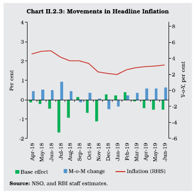 II.2.9 An early pre-monsoon uptick in food prices set in from March 2019 and returned food inflation to positive territory. With prices of fuel and light rising and partly offsetting the modest easing of inflation excluding food and fuel, headline inflation moved up to 2.9 per cent in March 2019. II.2.10 For the year 2018-19 as a whole, inflation eased by 17 bps from its level a year ago and by about 430 bps from its decennial average10. Households’ inflation expectations (median) moderated during the second half of 2018-19 by 160 bps for three months ahead and 170 bps for one year ahead horizons. A decline in inflation expectations is also corroborated by more forward-looking assessments by professional forecasters and in consumer confidence surveys. 4. Constituents of CPI Inflation II.2.11 The composition of CPI inflation underwent significant shifts during 2018-19 (Chart II.2.4). Subsequent paragraphs discuss the key drivers of the sharp decline in food inflation, the volatile nature of fuel inflation, and the sharp upturn in inflation excluding food and fuel during 2018-19 as well as its easing in the closing months of the year. Food II.2.12 Inflation in food and beverages prices (weight: 45.9 per cent in CPI) plunged during the year, with its contribution to overall inflation dropping to 9.6 per cent in 2018-19 from 29.3 per cent a year ago. Bumper production levels during 2016-18 muted the pre-monsoon uptick in April-August 2018 and food prices began declining from September 2018 and went into deflation during October 2018-February 2019 (Chart II.2.5). Several factors stand out in this remarkable easing: first, the extended winter easing in vegetables prices from December 2017 through April 2018; second, the unprecedented fall in prices of fruits from June 2018 up to January 2019; third, the unusual easing of inflation in respect of cereals, and milk and products during the second half of the year; fourth, continuing deflation in pulses and products prices; and fifth, sugar price deflation becoming more pronounced during the year. 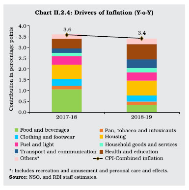 II.2.13 Drilling down into these key drivers, it is observed that as in the previous two years, prices of vegetables (weight: 13.2 per cent in CPI-food and beverages) became pivotal to the overall food inflation trajectory during 2018-19. The extended winter easing in vegetables prices was primarily driven by higher market arrivals of onions and tomatoes, aided by imports and the imposition of a minimum export price (MEP) for onions in November 2017. The pre-monsoon upturn in vegetables prices was less pronounced than in the past and was delayed till May 2018, but it peaked in July in sync with the historical pattern. Price pressures started easing from August, after which vegetables prices moved into contraction, led by a rise in market arrivals of potatoes, onions and tomatoes. A timely winter contraction in prices took overall food group prices into deflation from October 2018, which continued up to February 2019. Barring prices of tomatoes, which were impacted by delayed harvesting in Maharashtra, fungus led crop-damage in Karnataka and cyclone Gaja driven crop loss in Tamil Nadu, prices of onions, potatoes and other major vegetables remained soft, until sharp recovery set in during March 2019 (Chart II.2.6a). 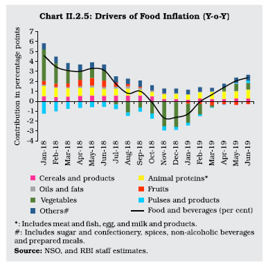 II.2.14 In the case of prices of fruits (weight: 6.3 per cent in CPI-food and beverages), summer upside pressures (April-May 2018) dissipated from June 2018 on account of robust domestic arrivals of mangoes and bananas (30.4 per cent of the total weight of CPI-fruits) and imports of apples and citrus fruits, and negative price momentum continued till January 2019. The downward trend in cumulative momentum from August 2018 defied the historical pattern and contributed considerably to the overall fall in food inflation during the year (Chart II.2.6b). Excluding vegetables and fruits, average food inflation would have been higher by around 92 bps at 1.6 per cent during 2018-19 (0.7 per cent including vegetables and fruits). 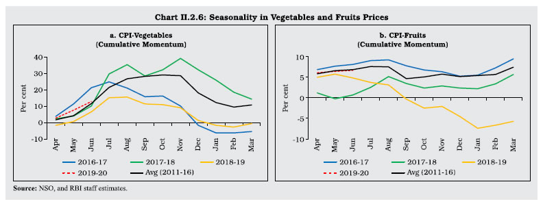
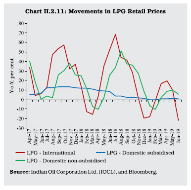
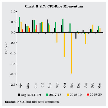 II.2.15 Among the other major food items, inflation in cereals and products prices (largest weight of 21.1 per cent in CPI-food and beverages), almost halved to 1.4 per cent in H2:2018-19. Notably, rice prices contracted for five consecutive months from September 2018, reflecting higher domestic production and adequate stocks (Chart II.2.7). The momentum of wheat prices generally remained strong during the year partly due to a fall in wheat imports caused by hike in import duty to 30 per cent in May 2018 from 20 per cent earlier. Inflation in milk and products prices (weight: 14.4 per cent in CPI-food and beverages) eased to 0.8 per cent in H2:2018-19 from 2.9 per cent in H1, reflecting adequate domestic availability (Chart II.2.8).  II.2.16 Deflation in prices of pulses (weight: 5.2 per cent in CPI-food and beverages) persisted through 2018-19 due to sizeable excess supply (Chart II.2.9). The negative contribution of pulses to overall inflation decreased from (-) 17.9 per cent during 2017-18 to (-) 5.7 per cent in 2018- 19 as mandi prices of arhar and urad edged towards their minimum support prices (MSPs). II.2.17 Prices of sugar and confectionery (weight: 3.0 per cent in CPI-food and beverages) remained in deflation since February 2018 reflecting excess supply conditions including increased open market sales. Domestic sugar prices have also closely tracked movements in global sugar prices. Price pressures in oils and fats (weight: 7.8 per cent in CPI-food and beverages) generally remained weak during the year in line with subdued international edible oils prices. Higher production of soybean and mustard during 2018-19 along with the reduction in import duty on crude palm oil, and refined, bleached and deodorised (RBD) palmolein imports from Malaysia and Indonesia, effective January 1, 2019, helped contain prices. II.2.18 Prices of protein-rich items such as meat and fish (weight: 7.9 per cent in CPI-food and beverages) faced some upside pressures during H2:2018-19, largely reflecting higher prices of maize, which is a key input for poultry and animal feed. Fuel II.2.19 The contribution of the fuel group (weight: 6.8 per cent in CPI) to headline inflation remained unchanged at the previous year’s level (11.3 per cent). Two distinct phases are discernible: first, a steep and sustained rise during H1:2018-19 to a peak of 8.6 per cent in September 2018; and second, a sharp softening in inflation during H2:2018-19 to touch a low of 1.2 per cent in February 2019. Domestic LPG and non-subsidised kerosene prices picked up during H1:2018-19 in line with the rise in international prices. Oil marketing companies also raised administered kerosene prices in a calibrated manner to phase out the kerosene subsidy. These dynamics, however, reversed during the second half of the year. The cumulative momentum in electricity prices began easing post-August 2018 and turned negative from November (Chart II.2.10). Firewood and chips price pressures remained muted throughout the second half of the year. Domestic LPG prices contracted during December 2018-February 2019, primarily tracking global LPG price movements (Chart II.2.11). 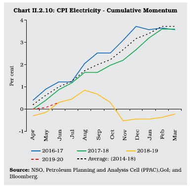
 Inflation Excluding Food and Fuel II.2.20 After remaining moderate at 4.6 per cent during 2017-18 (4.7 per cent during 2015-18), inflation excluding food and fuel surged to 5.8 per cent during 2018-19 (Appendix Table 4), with an intra-year peak of 6.4 per cent in June 2018 (highest since August 2014) (Chart II.2.12). In this category, the momentum of increase in prices of miscellaneous goods and services, which comprise 60 per cent of the category, was noteworthy. Within this sub-category, health and education prices surprised on the upside especially in rural areas during October- December 2018 and in respect of medicines, hospital and nursing home charges, prices of books and journals, and fees of private tutors and coaching centres. 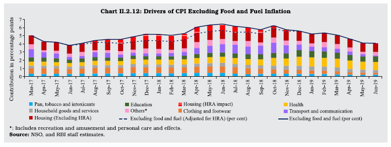 II.2.21 Among other items within the miscellaneous category, price pressures remained strong in respect of household goods and services, and transport and communication, the latter impacted by the increase in domestic petrol and diesel prices in line with international price movements (Chart II.2.13). In order to contain price pressures, the central government announced a cut in petrol and diesel prices by ₹2.5 per litre on October 4, 2018 by reducing excise duty by ₹1.5 per litre and asking oil companies to absorb ₹1.0 per litre. Several state governments also announced matching cuts by lowering local taxes. During November-December 2018, however, domestic petrol and diesel prices fell in line with international prices, thus containing transport and communication inflation. Prices of recreation and amusement – particularly, charges of cable television connection – and those of personal care and effects (particularly, prices of gold and silver and fast moving consumer goods like toiletries and cosmetics) posed upside pressures in February 2019. In March 2019, an unexpected softening in the momentum of housing prices, fall in gold prices and a favourable base effect pulled down inflation in the category as a whole. As a result, inflation excluding food and fuel fell from 6.2 per cent in October 2018 to 5.2 per cent in January 2019 and further to 5.1 per cent in March 2019, after a marginal uptick in February.  II.2.22 Net of housing, inflation excluding food and fuel averaged 5.6 per cent in 2018-19, up from 4.1 per cent in the previous year. The statistical impact of the increase in house rent allowance (HRA) for central government employees under the 7th Pay Commission started waning from July 2018 and dissipated completely by December 2018. Reflecting this, housing inflation followed a downward trajectory from July 2018 onwards to reach 4.9 per cent in March 2019, from a five-year peak of 8.5 per cent in April 2018. II.2.23 Clothing and footwear inflation also saw substantial easing to an intra-year low of 2.5 per cent in March 2019, reflecting the impact of lower export of readymade garments to UAE and Saudi Arabia subsequent to the imposition of a value added tax (VAT) of 5 per cent for the first time in January 2018. In terms of the Cotton A index, international prices of cotton, a major input into clothing production, also fell during the major part of the year (particularly July 2018-February 2019) barring some recovery in March 2019. 5. Other Indicators of Inflation II.2.24 During 2018-19, sectoral CPI inflation based on Consumer Price Index of Industrial Workers (CPI-IW) increased significantly to 7.7 per cent in March 2019 from 4.0 per cent in April 2018, largely due to housing. The housing index under the CPI-IW is adjusted twice a year – in January and July (in contrast to the continuous adjustment under CPI-Combined). Inflation based on the Consumer Price Index of Agricultural Labourers (CPI-AL) and the Consumer Price Index of Rural Labourers (CPI-RL), which do not have housing components, eased during June-November 2018 before picking up during December 2018-March 2019. II.2.25 Inflation measured by the Wholesale Price Index (WPI) showed mixed movements during 2018-19. It reached an intra-year peak of 5.7 per cent in June 2018 due to price pressures emanating from all the three major groups (i.e., primary articles, fuel and power, and manufactured products) before easing to 4.6 per cent in August 2018. It picked up again during September-October 2018, driven by a sharp uptick in prices of all three major groups, however, it moderated to 3.1 per cent in March 2019, led by a significant softening of price pressures in fuel and power during November 2018-January 2019, which track international prices. On an annual average basis WPI inflation picked up to 4.3 per cent in 2018-19 from 2.9 per cent in 2017-18. A similar rising trend was also visible in the GDP deflator, which picked up to 4.1 per cent in 2018-19 from 3.8 per cent in 2017-18. II.2.26 Major increases in MSPs were announced during 2018-19 for kharif crops, in line with the provisions of the Union Budget, 2018-19, to ensure at least 50 per cent return over costs (A2+FL)11. As a result, MSP of paddy (common) was hiked by 12.9 per cent (from ₹1,550 per quintal in 2017-18 to ₹1,750 per quintal in 2018- 19). The extent of MSP increases varied across crops, ranging from 3.7 per cent in the case of urad to 52.5 per cent for ragi. While the impact of MSP increases was reflected in mandi prices of many crops, there was no commensurate increase in consumer prices owing to abundant domestic availability across major food items. Secondary data reveal that mark-ups (i.e., the difference between retail and mandi prices) vary across crops and over time (Chart II.2.14). In view of data gaps impeding a full tracking of wholesale/mandi price changes into retail inflation, a primary survey was undertaken to understand the behaviour of multi-stage margins over the supply chain for key agricultural commodities in India (Box II.2.1). II.2.27 Wage growth for agricultural and non-agricultural labourers generally remained subdued during the year, averaging around 4.0 per cent, reflecting low food inflation. In the case of the corporate sector, pressures from staff costs largely remained range-bound during the year. II.2.28 In sum, headline inflation softened during 2018-19, mainly reflecting significantly low food inflation. With the domestic and global demand-supply balance of key food items expected to remain favourable, the short-term outlook for food inflation remains benign. Spike in vegetables prices from their lows in 2018-19, especially during the summer months, poses some upside risk. The spatial and temporal distribution of monsoon will have a bearing too, although the recent catch-up in rainfall may likely mitigate the risk. The outlook for global crude oil prices is hazy, both on the upside and downside. Should the recent slowdown in domestic economic activity accentuate, it may have a bearing on the outlook for inflation. 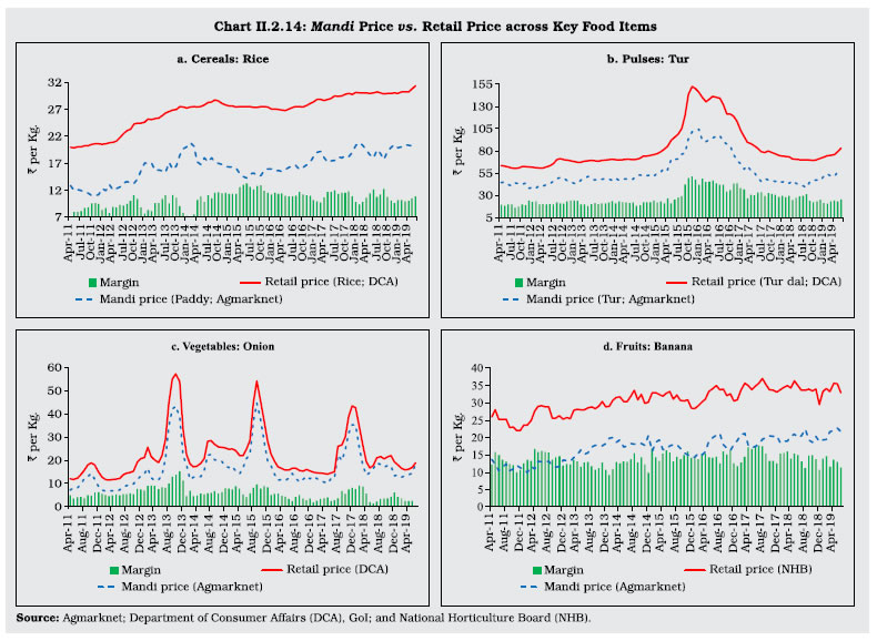
Box II.2.1
Supply Chains and Food Inflation Dynamics In India, food inflation underwent sustained moderation from 2014-15 (Chart 1). Excess supply conditions relative to demand engendered by successive bumper production during 2016-18 have structurally dampened inflationary impulses (please see Box II.1.4). Alongside, improvements in supply chain dynamics – wider road networks; low cost access to mobile phones enabling easier flow of information between deficit and surplus centres; speedier movement of shipments in the post-GST common market; financial inclusion and spread of micro-finance enabling easier access to working capital for small traders and retailers – may also have contributed to this sustained moderation. Available empirical research highlights the influence of mark-ups between farm-gate and retail prices in explaining food inflation and its volatility (Bhattacharya, 2016). Literature also highlights that in the absence of government intervention, behaviour of traders and big retailers could aggravate inflationary impact of a negative supply shock (Lahiri and Ghosh, 2014). A pan-India survey was conducted in December 2018 to understand supply chain dynamics in the context of the sustained moderation in food inflation. The survey covered a total of 9,403 respondents comprising farmers (2,811), traders (3,184) and retailers (3,408) spread across consumption and production centres (Table 1). It was conducted in 85 mandis spread across 16 states covering 16 major kharif food crops which form part of the CPI food basket. | Table 1: Survey Coverage | | Mandi/Centre | Group/Commodities | | Respondents | Consumption Centres | Production Centres | Total | Major Groups | Commodities | | | | | | Cereals | Paddy/Rice | | Farmers | 1,147 | 1,664 | 2,811 | Pulses | Tur, Moong, Urad, Bengal gram | | Traders | 2,176 | 1,008 | 3,184 | Oilseeds | Groundnut, Soybean | | Retailers | 2,356 | 1,052 | 3,408 | Vegetables and fruits | Onion, Potato, Tomato, Green chillies, Brinjal, Apple, Banana, Coconut | | Total | 5,679 | 3,724 | 9,403 | Spices | Turmeric, Red chillies | The findings revealed that farmers’ share in retail prices vary between 28-78 per cent across 14 crops12 – lower in the case of perishables (vegetables) and higher for non-perishables (oilseeds and spices). Mark-ups are influenced by a number of factors – commissions and mandi charges; loading/unloading charges; packing, weighing and assaying charges; transport costs; shop rentals and local taxes; storage costs and membership fees. Cash was reported as the dominant mode of transactions in mandis, with its share ranging between 84-93 per cent. Further, it was found that retailers’ margins are generally higher than the traders’ margins in consumption centres, due to significant product loss at the marketing stage, particularly for perishables. 62 per cent of farmers revealed that their selling prices were higher than their production costs. As regards government policies, minimum support prices (MSPs) and readily available market information are helpful to farmers in realising better prices. Farmers also revealed that reliable weather forecasts, improved storage facilities and government advisory on crops could help them take better cropping decisions. A majority of the traders viewed that improving storage facility and allowing free trade is important, while most retailers believed that government intervention and better availability of information could help in arresting price rise. Using the survey data, the following multivariate regression equation was estimated by the Ordinary Least Squares (OLS) method, pooling data across crops and states: The results indicate that improvement in infrastructure such as tele-density (per 100 persons), road density and number of wholesale markets to gross cropped area reduce mark-ups of both traders and retailers. Furthermore, while increase in per capita income influences traders’ mark-up positively, literacy rate influences retailers’ mark-up negatively. On the whole, multi-stage mark-ups across crops play an important role in determining the trajectory of food inflation. Surveys can play an important role in gauging the interaction between traders and retailers in mark-up formation during periods of shifts in food inflation behaviour. References: 1. Lahiri, H., and A. N. Ghosh (2014), ‘Government’s Role in Controlling Food Inflation’, in Ghosh, A., and A. Karmakar (eds.) Analytical Issues in Trade, Development and Finance, India Studies in Business and Economics, Springer India. 2. Bhattacharya, R. (2016), ‘How does Supply Chain Distortion Affect Food Inflation in India’, NIPFP Working Paper Series, No. 173. | II.3 MONEY AND CREDIT II.3.1 During 2018-19, monetary and credit conditions aligned with their pre-demonetisation trends and they increasingly reflected underlying macroeconomic and financial developments, often with lead information content. Reserve Money (RM), which had expanded robustly in 2017-18 on the back of a surge in new currency into circulation, reverted to long-term trend growth in 2018-19. In the process, India’s currency-GDP ratio increased to 11.2 per cent in 2018-19 from 10.7 per cent a year ago with the expansion matched by liquidity injection through LAF operations as well as outright open market purchases among the sources of reserve money and reflected in net domestic assets in the form of net RBI credit to the Government. By contrast, the RBI’s foreign exchange interventions drained liquidity during the year. II.3.2 Broad Money picked up further in 2018-19, leaving behind a prolonged 10-year deceleration14. Deposit growth, has firmed up steadily from December 2017, albeit from a secular slowdown that commenced in August 2009. Credit growth turned up ahead of deposit growth i.e., from November 2017 as appetite for lending to the commercial sector improved, especially to less-financially stressed sectors of the economy like households and services along with infrastructure, and subsequently the credit to GDP gap narrowed. The overall brightening of the credit climate compensated for the decline in non-bank sources of resource flow and boosted the total flow of resources to the commercial sector. II.3.3 In this milieu, immediately following sub-section on RM brings to the fore, developments pertaining to cash intensity and digital transactions, and the re-emergence of net RBI credit to the government as the largest source of expansion during the year. The follow-up sub-section 3 on money supply indicates recovery in deposit growth and steady increase in credit growth. The credit growth story at both macro and sectoral levels has been covered in sub-section 4. 2. Reserve Money II.3.4 RM which is essentially an analytical and stylised presentation of the balance sheet of the RBI, focuses on the monetary liabilities of the Reserve Bank. Expanding at 14.5 per cent in 2018-19, it stood a little below its decennial trend (14.6 per cent during 2007-16) after a hiatus in 2016-17 representing the impact of demonetisation (Chart II.3.1; Appendix Table 4). RM growth was 13.5 per cent as on June 28, 2019. II.3.5 In terms of its components, 87 per cent of expansion in RM in 2018-19 took the form of currency in circulation (CiC). The usual seasonal spurt in currency demand in Q1- associated with festivals, rabi procurement and kharif sowing - gave way to a seasonal contraction in the next quarter as cash returned to the system with the ebbing of agricultural activity. Thereafter, however, CiC expanded almost monotonically as cash demand for the kharif harvest and festivals in Q3, and the rabi harvest crops beginning in Q4 was amplified by election-related spending. In spite of CiC growth of 16.8 per cent for the year as a whole, the currency-GDP ratio remained lower than 11.6-12.2 per cent observed during 2011-2016, perhaps indicating decline in cash intensity of the economy (Chart II.3.2a). The space vacated by cash appears to have been occupied by retail digital payments (Chart II.3.2b). 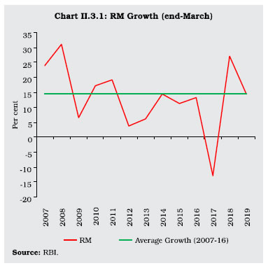
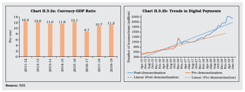 II.3.6 Bankers’ deposits with the Reserve Bank, the other major component of RM15, remained broadly stable during the year. Nonetheless, higher deposit mobilisation and an unchanged CRR caused them to grow by 6.4 per cent, faster than 3.9 per cent in the previous year. With active liquidity management operations by the Reserve Bank including front-loaded measures to help market participants through the ‘year-end balance sheet’ phenomenon, banks’ demand for excess reserves has been steadily declining over recent years (Chart II.3.3). II.3.7 Amongst the sources, net domestic assets (NDA) and net foreign assets (NFA) underwent compensating variations, unlike in the preceding year when the large increase in RM was driven by an expansion in both (Chart II.3.4). Within NDA, net RBI credit to the government contributed 93 per cent of the expansion in RM in 2018-19, boosted by liquidity injections through open market operations (OMO) to the tune of ₹3.0 trillion and a decline in cash balances of the government with the RBI of the order of ₹0.4 trillion. The OMO purchases which began from May 2018, intensified in the subsequent months throughout the year, barring August. The other constituent of NDA i.e., net claims on banks and the commercial sector, by way of LAF operations smoothened transient liquidity mismatches, increasing by ₹895 billion over their level in the previous year. Two distinct phases, in their operations were evident; persisting reverse repo mode in Q1 and most part of Q2 to mainly drain away the liquidity slosh in the system due to government spending; and largely repo mode in the rest of the year as liquidity conditions tightened sharply under the impact of forex sales and currency leakage. Notably, system liquidity experienced shortages despite injection of durable liquidity through OMOs of the order of ₹3.0 trillion, the highest in any year so far. 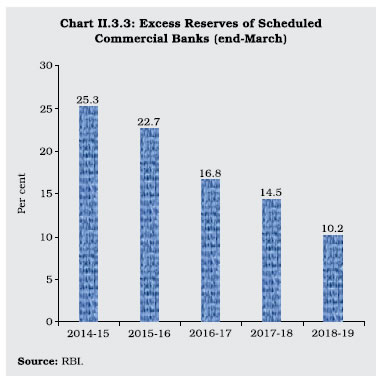
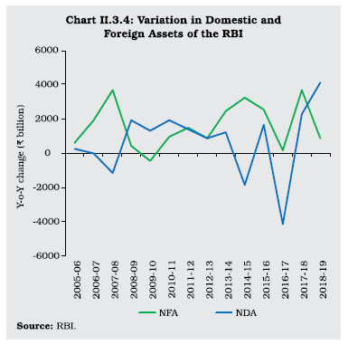 II.3.8 By contrast, NFA was impacted by the Reserve Bank’s intervention in the foreign exchange market, with net sales of foreign currency to authorised dealers of ₹1.12 trillion (purchases of ₹2.23 trillion a year ago). This depletion was, however, counter balanced by increase in aid receipts, net interest/discount earned, gold and valuation gains. During the year, the Reserve Bank augmented its liquidity management toolkit by injecting rupee liquidity for longer duration through long-term foreign exchange buy/sell swap. In March 2019, the Reserve Bank undertook USD/INR swaps of US$5 billion with a maturity of three years to inject rupee liquidity, which also recouped some of NFA losses during the year. 3. Money Supply II.3.9 Money supply, measured by the broad monetary aggregate or M3, expanded at steady pace, its growth rate averaging 10.2 per cent during the year, after having fallen to a historic low of 5.6 per cent in September 2017. M3 growth stood at 10.1 per cent as on June 21, 2019. II.3.10 Among the components, aggregate deposits (ADs) grew by 9.6 per cent (5.8 per cent in the previous year) and accounted for 80 per cent of the increase in M3 during the year (Chart II.3.5). An upturn in the momentum of time deposits (TDs), the major constituent of ADs, started in Q4 of 2017-18 and was strong enough to overcome unfavourable base effects so as to persist through 2018-19, co-moving with interest rates on these deposits (Chart II.3.6). Decomposition of aggregate deposits into trend and cyclical components reveals the predominance of the latter. As usual, demand deposits remained volatile and moved in lateral inversions of variations in currency with the public (Chart II.3.7). In the event, demand deposits expanded faster than in the preceding year. The growth of currency with the public stabilised at 16.6 per cent during the year after the post-demonetisation surge of 39.2 per cent in the previous year. 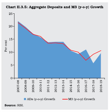
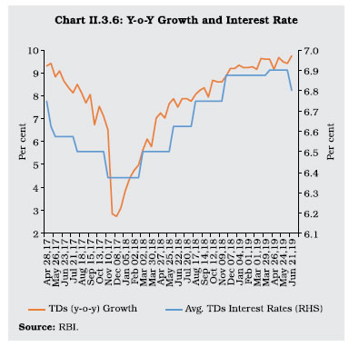 II.3.11 From the sources side, bank credit to the commercial sector accounted for 79 per cent of the expansion in M3 during 2018-19 (Chart II.3.8 and Table II.3.1). After its prolonged deceleration, the recovery in credit growth started during the later part of 2017-18 and got entrenched on the back of robust lending to services sector and in the form of personal loans. Net bank credit to government increased during 2018-19 essentially due to higher net credit from the Reserve Bank, as alluded to earlier, even as commercial banks’ investment in government securities grew modestly. Net foreign exchange assets of the banking sector decelerated, reflecting sales of foreign exchange by the Reserve Bank as explained in the preceding sub-section. 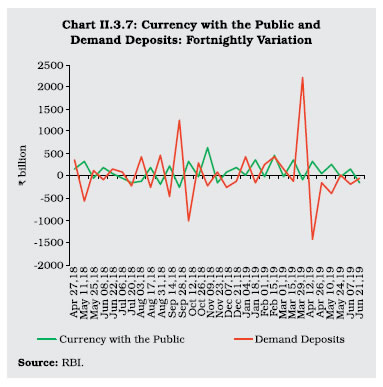
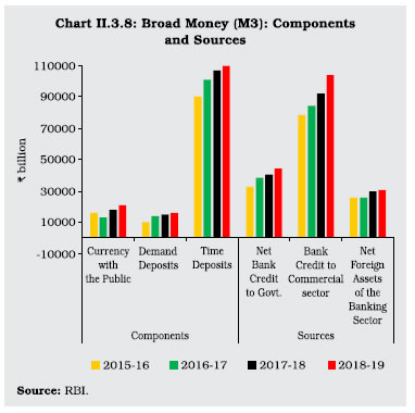
| Table II.3.1: Monetary Aggregates | | Item | Outstanding as on March 31, 2019
(₹ billion) | Year-on-year Growth (per cent) | | 2017-18 | 2018-19 | 2019-20
(as on June 21) | | 1 | 2 | 3 | 4 | 5 | | I. Reserve Money | 27,705 | 27.3 | 14.5 | 13.5 | | II. Broad Money (M3) | 154,309 | 9.2 | 10.5 | 10.1 | | III. Major Components of M3 | | | | | | 1. Currency with the Public | 20,522 | 39.2 | 16.6 | 12.8 | | 2. Aggregate Deposits | 133,469 | 5.8 | 9.6 | 9.6 | | IV. Major Sources of M3 | | | | | | 1. Net Bank Credit to Government | 43,878 | 3.8 | 9.7 | 8.7 | | 2. Bank credit to Commercial Sector | 103,802 | 9.5 | 12.7 | 11.5 | | 3. Net Foreign Exchange Assets of the Banking Sector | 30,708 | 14.2 | 5.1 | 10.4 | | V. M3 net of FCNR(B) | 152,706 | 9.2 | 10.5 | 10.1 | | VI. M3 Multiplier | 5.6 | | | | Note: 1. Data are provisional.
2. The latest data for RM pertains to June 28, 2019.
Source: RBI. | Key Monetary Ratios II.3.12 The key behavioural parameters that drove the formation of monetary aggregates converged gradually towards their pre-demonetisation (2008-16) trends during 2018-19. With the pace of expansion in currency running above trend on a combination of factors (addressed in sub section 2) and significantly ahead of deposit growth, the currency-deposit (C/D) ratio rose in 2018-19 to levels last recorded during the pre-demonetisation (2008-16) phase indicative of persisting structural liquidity tightness. The money multiplier (MM), which measures the expansionary/contractionary effects of the Reserve Banks’ balance sheet on money supply in the economy, underwent three distinct phases in a historical perspective. A rising trend during 1950-75 (from 1.5 to 3.0) characterised the period, reflecting monetary accommodation as money demand for investment driven growth in the economy was amplified by nationalisation of banks and establishment of all India financial institutions (Chart II.3.9). This was followed by a stable period till 1995 as a result of the weakening pace of deposit mobilisation due to near stagnancy in per capita income growth. Thereafter an increasing phase set in that has extended till date propelled, inter alia, by the step-up in the demand for money associated with a higher growth trajectory, visitations of capital flows and a reduction in reserve ratios – in fact, structural break in the path of the MM is detected in June 1999. As on June 21, 2019, MM stood at 5.6 same as in the previous year. II.3.13 The reserve-deposit (R/D) ratio is shaped by regulatory norms – an increase in R/D restrains money supply and vice versa, and conveys the stance of monetary policy. Not surprisingly, therefore, it is a stable ratio, hovering between 0.04-0.06 except during 1975-2000 when monetary policy essentially relied on reserve requirements in its counter cyclical role of reining in the expansionary effects of fiscal activism. The C/D ratio which captures the public’s preference for cash vis-à-vis banking habits, is inversely related to MM. Over the years, the C/D ratio has been consistently declining, pointing to the expanding reach of banking services consequent upon nationalisation in 1969 and in 1980, financial inclusion and literacy, emphasising rural/unbanked areas and innovations in payment and settlement which have reduced cash dependence. 4. Credit II.3.14 SCBs’ credit to the commercial sector steadied during the year and rose by 13.3 per cent on March 31, 2019 (10.0 per cent a year ago) from a historic low of 3.7 per cent in March 2017. Double digit credit growth was recorded from December 2017, with a recent peak of 15.1 per cent in November 2018. Several supply side developments provided a congenial environment for credit growth to firm up and sustain - some reduction in balance sheet stress; recapitalisation of public sector banks (PSBs); calibrated reduction in SLR morphed into the liquidity coverage ratio (LCR); growing traction in the IBC process; and aggressive efforts towards asset recoveries/write-off/sales as well as provisioning. These developments underscore the critical role of availability of sufficient capital in enhancing credit growth (Box II.3.1). SCBs’ credit growth stood at 12.0 per cent as on June 21, 2019 (12.8 per cent a year ago). II.3.15 Credit growth was mainly driven by momentum, despite unfavourable base effects during 2018-19 (Chart II.3.10), and was supported by higher mobilisation of deposits during the year. This eventually resulted in a reduction in the incremental credit-deposit ratio from unusually high levels a year ago (Chart II.3.11). The credit-to-GDP gap has been narrowing from its recent peak in June 2017 though it remains negative, implying scope for further increase in credit growth without overheating (Chart II.3.12). II.3.16 As on March 31, 2019, non-food credit (NFC) rose 12.3 per cent over 8.4 per cent a year ago, driven mainly by flows to large-scale industry and the services sector. Among bank groups, credit extended by PSBs accelerated to 9.6 per cent in March 2019 from 5.3 per cent a year ago. Credit growth by private sector banks accelerated to 19.9 per cent from 18.7 per cent a year ago, benefiting from their niche orientation towards personal loans which are also stress-lite (Chart II.3.13). Box II.3.1
Role of Capital in Bank’s Lending Behaviour India’s banking sector has been beset by a large overhang of balance sheet stress which, in turn, contributed to a slowdown in credit growth. In addition, the phased implementation of Basel III and higher provisioning requirements significantly expanded capital requirements. Typically, information asymmetries in the credit market and especially, imperfect information availability pushes up the cost of borrowings of capital starved banks in view of poor substitutability between retail deposits and wholesale funding (Kashyap and Stein, 1995). These constraints tend to ease for sufficiently capital endowed banks. A well-capitalised bank may also face lower risk premium while borrowing from the capital market (Gambacorta and Shin, 2018). A panel Generalised Method of Moments (GMM) model estimated on annual data for 30 banks16 from 2008-09 to 2017-18 reveals that an increase in leverage leads to a rise in cost of funds. On the other hand, higher CRAR is found to reduce the cost of funds for banks. Credit growth decreases with an increase in cost of funds and NPAs. On the other hand, it increases as CRAR rises - one percentage point increase in the CRAR results in loan growth rising by 3 percentage points. References: 1. Gambacorta, L., and Shin, H. S. (2018). Why Bank Capital Matters for Monetary Policy. Journal of Financial Intermediation, 35, 17-29. 2. Kashyap, A. K., and Stein, J. C. (1995). The Impact of Monetary Policy on Bank Balance Sheets. Carnegie-Rochester Conference Series on Public Policy (Vol. 42, pp. 151-195). North-Holland. | 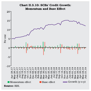
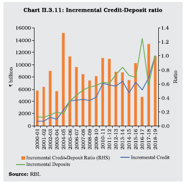
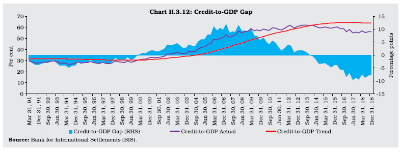 Sectoral Credit Deployment by Banks II.3.17 Credit growth to agriculture accelerated to 7.9 per cent in March 2019 from 3.8 per cent a year ago, driven by foodgrains and horticulture production (Table II.3.2). Credit to industry accelerated to 6.9 per cent in March 2019 from 0.7 per cent in March 2018. Within industry, a pick-up in credit was reasonably broad-based but accentuated towards infrastructure; engineering; cement and cement products; glass and glassware; construction; and chemical and chemical products. Credit to infrastructure, in particular, accelerated to 18.5 per cent in March 2019 as against a contraction of 1.7 per cent last year, driven largely by higher credit offtake by roads and power segments, urban transport, affordable housing and renewable energy. On the other hand, credit to some segments, viz., basic metal and metal products; and textiles decelerated/contracted reflecting persisting stress. II.3.18 Credit to the services sector maintained double-digit growth and expanded by 17.8 per cent by end-March 2019 as compared with 13.8 per cent a year ago, pulled up mainly by non-banking financial companies (NBFCs). Credit growth to other segments, viz., wholesale trade, commercial real estate and transport operators also accelerated. Personal loans growth remained healthy, although it moderated to 16.4 per cent by end-March 2019 from 17.8 per cent a year ago, pulled down by deceleration in vehicle and education loans. 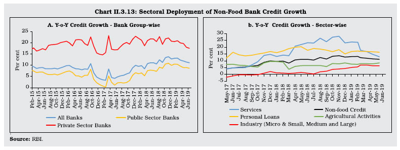
| Table II.3.2: Credit Deployment to Select Sectors | | Sectors | Outstanding as on March 29, 2019 | Year-on-Year Growth (per cent) | | (₹ billion) | 2017-18* | 2018-19# | 2019-20## | | 1 | 2 | 3 | 4 | 5 | | Non-food Credit (1 to 4) | 86,334 | 8.4 | 12.3 | 11.1 (11.1) | | 1. Agriculture & Allied Activities | 11,113 | 3.8 | 7.9 | 8.7 (6.5) | | 2. Industry (Micro & Small, Medium and Large) | 28,858 | 0.7 | 6.9 | 6.4 (0.9) | | 2.1. Micro & Small | 3,755 | 0.9 | 0.7 | 0.6 (0.7) | | 2.2. Medium | 1,064 | -1.1 | 2.6 | 2.2 (2.7) | | 2.3. Large | 24,039 | 0.8 | 8.2 | 7.6 (0.8) | | (i) Infrastructure | 10,559 | -1.7 | 18.5 | 15.2 (0.0) | | of which: | | | | | | (a) Power | 5,690 | -1.1 | 9.5 | 9.7 (-1.2) | | (b) Telecommunications | 1,156 | -0.6 | 36.7 | 20.9 (6.8) | | (c) Roads | 1,869 | -7.5 | 12.2 | 14.6 (-5.7) | | (ii) Chemicals & Chemical Products | 1,915 | -5.5 | 17.5 | 11.1 (2.3) | | (iii) Basic Metal & Metal Product | 3,716 | -1.2 | -10.7 | -10.3 (-5.5) | | (iv) Food Processing | 1,571 | 6.8 | 1.1 | 1.2 (3.3) | | 3. Services | 24,156 | 13.8 | 17.8 | 13.0 (23.3) | | 4. Personal loans | 22,207 | 17.8 | 16.4 | 16.6 (17.9) | | 5. Priority Sector | 27,390 | 4.8 | 7.3 | 10.2 (6.3) | *: March 2018 over March 2017.
#: March 2019 over March 2018.
##: June 2019 over June 2018.
Figures in brackets indicate growth rates in June 2018 over June 2017.
Note: Data are provisional and relate to select banks which cover about 90 per cent of total non-food credit extended by all scheduled commercial banks.
Source: RBI. | II.3.19 During Q1:2019-20, non-food credit maintained double digit growth on a y-o-y basis as in the previous year. Sector-wise, credit to both ‘agriculture & allied activities’ and ‘industry’ accelerated to 8.7 per cent (6.5 per cent last year) and 6.4 per cent (0.9 per cent last year) respectively, while credit to the services sector moderated to 13.0 per cent (23.3 per cent last year) in June 2019. It is noteworthy that credit growth to infrastructure sector recovered sharply to 15.2 per cent in June 2019 mainly due to strong credit flow to power, telecommunications and roads sectors. Flow of Financial Resources to Commercial Sector II.3.20 During 2018-19, there has been an improvement in the total flow of financial resources to the commercial sector, which increased by 4.2 per cent on a year-on-year basis (Table II.3.3). While flows from non-banks declined, flows from banking sources, i.e., non-food bank credit recorded an increase and met the financing requirements of the commercial sector. II.3.21 The decline in flows from non-banks was mainly on account of lower flows from non-deposit taking systemically important NBFCs (net of bank credit to NBFCs) and housing finance companies, particularly in the aftermath of IL&FS event. Moreover, lower issuances of debt and equity instruments by non-financial entities and lower investment by LIC in corporate debt, infrastructure and social sector also resulted in lowering financial flows in 2018-19 from their levels a year ago. In contrast, there was a sharp increase in commercial paper issuances, coupled with higher accommodation by four All India Financial Institutions (AIFIs) regulated by the Reserve Bank. Among foreign sources, external commercial borrowings (ECB)/foreign currency convertible bonds (FCCB) recorded net inflows for the first time in the last four years. FDI flows, which account for a major share of non-bank finance to the commercial sector, increased by 18.9 per cent. On the other hand, short-term credit from abroad declined during the year as import growth decelerated. | Table II.3.3: Flow of Financial Resources to Commercial Sector | | (₹ Billion) | | Source | April - March | April - June | | 2016-17 | 2017-18 | 2018-19 | 2018-19 | 2019-20 | | 1 | 2 | 3 | 4 | 5 | 6 | | A. Adjusted non-food Bank Credit | 4,952 | 9,161 | 12,300 | -182 | -1,764 | | i) Non-Food Credit | 3,882 | 7,959 | 11,467 | -316 | -1,530* | | of which: petroleum and fertiliser credit | 133 | 27 | 75 | -46 | -143 | | ii) Non-SLR Investment by SCBs | 1,070 | 1,202 | 833 | 133 | -235* | | B. Flow from Non-banks (B1+B2) | 9,547 | 11,603 | 9,342 | 2,837 | 2,441 | | B1. Domestic Sources | 6,789 | 8,219 | 5,474 | 2,266 | 1,429 | | 1. Public issues by non-financial entities | 155 | 438 | 106 | 39 | 533 | | 2. Gross private placements by non-financial entities | 2,002 | 1,462 | 1,505 | 268 | 351 | | 3. Net issuance of CPs subscribed to by non-banks | 1,002 | -254 | 1,361 | 1,233 | 191 | | 4. Net Credit by housing finance companies | 1,374 | 2,198 | 1,465 | 412 | 143@ | | 5. Total accommodation by 4 RBI - regulated AIFIs - NABARD, NHB, SIDBI & EXIM Bank | 469 | 950 | 1,136 | 274 | 115 | | 6. Systemically important non-deposit taking NBFCs (net of bank credit to NBFCs) | 1,510 | 3,046 | -397 | | | | 7. LIC’s net investment in corporate debt, infrastructure and social sector | 277 | 378 | 300 | 40 | 96 | | B2. Foreign Sources | 2,758 | 3,385 | 3,867 | 571 | 1,012 | | 1. External Commercial Borrowings / FCCB | -509 | -51 | 696 | -101 | 396 | | 2. ADR/GDR Issues excluding banks and financial institutions | - | - | - | - | - | | 3. Short-term Credit from abroad | 435 | 896 | 152 | | | | 4. Foreign Direct Investment to India | 2,833 | 2,540 | 3,019 | 672 | 616@ | | C. Total Flow of Resources (A+B) | 14,500 | 20,764 | 21,642 | 2,655 | 677 | | Memo: Net resource mobilisation by Mutual Funds through Debt (non-Gilt) Schemes | 1,206 | -59 | -1,211 | -383 | -148 | @: Up to May 2019.
*: Data pertain to the period April-June 21, 2019.
Note: (i) Due to change in categorisation of mutual fund schemes by SEBI, data on net resource mobilisation by mutual funds through debt (non-gilt) schemes from April 1, 2019 onwards may not be comparable with previous years’ data. | II.3.22 To sum up, the monetary aggregates and the behavioural ratios pointed to underlying economic activity gaining resilience although it is important to note that this improvement is set against the backdrop of a slowdown that began since 2010-11. Credit conditions improved through both demand and supply side factors. Progress in capitalisation and initiatives to resolve stressed assets facilitated higher credit offtake from PSBs. Sector-wise, sustained growth of credit to services along with restarting of industrial credit flows was the notable feature of the steady improvement in the appetite of banks to lend during 2018-19. The total flow of resources to the commercial sector, led by banks, recorded an increase. II.4 FINANCIAL MARKETS II.4.1 Global financial markets turned volatile for most part of 2018-19 as global spillovers in the form of monetary policy normalisation in the US, trade frictions and elevated crude oil prices triggered risk aversion towards emerging market economies (EMEs) as an asset class, sparking sell-off in financial assets and currency depreciations in these economies, as investors scrambled to safe havens. Towards the later part of the year, however, signs of slowdown in global growth and trade prompted accommodative monetary policy stances by major central banks. With receding trade war fears and easing of crude oil prices providing tailwinds, risk appetite returned during the last quarter of the year allowing financial markets to regain poise and post sporadic rallies, especially in EMEs. Currencies that had suffered losses due to the general strengthening of the US dollar also managed to recoup some losses and traded with an appreciating bias, barring those impacted by country-specific idiosyncratic factors. II.4.2 Indian equity markets exhibited resilience in the face of the EME-wide sell-off until August 2018 before plummeting in September 2018 with the unfolding of the credit event pertaining to Infrastructure Leasing & Financial Services Limited (IL&FS), a systemically important non-deposit accepting core investment company (CIC-ND-SI) registered with the Reserve Bank. Sentiment was adversely impacted by a series of defaults by IL&FS in repayments of commercial papers (CPs), non-convertible debentures (NCDs) and bank loans and the subsequent rating downgrades of IL&FS and a few other NBFCs. In the currency market, the Indian rupee depreciated tracking other EME currencies but the ebbing of global risks brought back portfolio flows in H2:2018-19. In the money market, as discussed in sub-section 2, overnight money market rates remained aligned with the policy repo rate, with active liquidity management by the Reserve Bank providing buffers in the context of adverse global developments. In the domestic bond market, G-sec yields hardened during H1:2018-19 on the back of increase in crude oil prices, rise in the US Treasury yields and sustained foreign portfolio outflows. In H2:2018-19, the trend reversed on account of easing of crude oil prices, enhanced open market operation (OMO) purchase auctions by the Reserve Bank and decline in US Treasury yields, as discussed in sub-section 3. Sub-section 4 presents developments in the corporate bond market. Sub-section 5 discusses developments in domestic equity market. Sub-section 6 profiles the rupee’s recovery in the foreign exchange market in H2:2018-19 after bouts of downward pressures in the first half of the year. 2. Money Market II.4.3 The money market remained generally stable during 2018-19 barring episodes of volatility in the commercial paper (CP) and certificates of deposit (CD) markets in the first and third quarter. Liquidity conditions altered gradually from surplus during Q1:2018-19 to deficit during rest of the year. The Reserve Bank proactively managed frictional liquidity conditions through both variable and fixed rate repos and reverse repos of various tenors, along with 14-day variable rate repos and recourse to the marginal standing facility (MSF). In order to address durable liquidity shortages caused by the Reserve Bank’s forex interventions and the expansion in currency in circulation, the Reserve Bank conducted outright purchase of government securities through OMOs. Furthermore, the Reserve Bank augmented its liquidity management toolkit towards the close of the year by adding long-term foreign exchange buy/sell swaps as an instrument to inject rupee liquidity for longer durations. II.4.4 The weighted average call rate (WACR) in the unsecured inter-bank call money market remained aligned with the policy repo rate through the year, albeit with a downward bias (Chart II.4.1). The negative spread of the WACR over the policy rate averaged 8 basis points (bps) but narrowed as liquidity conditions gradually tightened in the H2:2018-19. 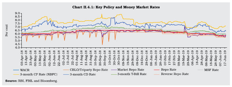 II.4.5 Even as spreads narrowed, volatility in the call money segment, measured by the standard deviation17 of the WACR, increased moderately over its level a year ago, especially in the H1:2018-19, reflecting the swings in liquidity conditions. In the overnight segment of the money market, the share of call money and triparty repo increased whereas the share of market repo declined, especially after the introduction of triparty repo on November 5, 2018 in place of the Collateralised Borrowing and Lending Obligation (CBLO). Borrowings in triparty repo have been exempted from maintenance of the cash reserve ratio (CRR), like borrowings in the market repo segment. During 2018-19, the CBLO/triparty repo and market repo rates remained below the WACR, on average, by 9 bps and 2 bps, respectively. II.4.6 Average daily volume in the money market (call money, CBLO/triparty repo and market repo taken together) increased by 12 per cent to ₹1,895 billion during 2018-19 from ₹1,687 billion in 2017-18. Volumes in the CBLO/triparty repo and market repo segments increased by 14 per cent and 5 per cent, respectively, to account for 64 per cent and 27 per cent, respectively, of the total overnight money market volume during 2018-19 as compared with 63 per cent and 29 per cent, respectively, in 2017-18. In the call money segment too, volumes increased by 29 per cent during the year, raising its market share to 9 per cent from 8 per cent a year ago. II.4.7 Interest rates on longer tenor money market instruments, viz., 3-month Treasury Bills (T-Bills), CDs and CPs generally moved in sync during 2018-19. However, the spread of CP and CD rates over T-Bill rate widened during the Q1:2018-19 until the first week of June 2018 (Chart II.4.2) on account of higher fund raising to meet the liquidity coverage ratio (LCR) requirement. Spreads subsided after LCR carve-out from the statutory liquidity ratio (SLR) was increased in June 2018 monetary policy review which reduced the demand for bulk deposits. Consequent to the IL&FS episode, CP spreads widened again in September until mid-November and were also impacted by the tightening of liquidity conditions.  II.4.8 In the primary market, fresh issuance of CDs increased to ₹5,653 billion during 2018-19 as compared with ₹4,403 billion a year ago. Issuance of CPs also increased to ₹25,964 billion in 2018-19 from ₹22,925 billion in 2017-18, mainly by private corporates and non-bank financial companies (NBFCs). The weighted average discount rates in the primary CP market, which hardened from September until mid-November on account of increased risk perception resulting from the IL&FS episode, softened thereafter till the end of March 2019 as risks subsided. II.4.9 During Q1:2019-20, money market remained stable with WACR being aligned with the policy repo rate. Liquidity condition, as reflected by the daily net LAF positions, turned into surplus mode in June 2019 mainly on the back of surge in the Government spending and injection of durable liquidity by the Reserve Bank. The Government also resorted to the Ways and Means Advances (WMA). 3. G-sec Market II.4.10 The aggregate volume of transactions in central government and state governments dated securities (G-secs and SDLs) and T-Bills (outright as well as repo) declined by 5.7 per cent during 2018-19. In Q1, the G-sec yields hardened by 51 bps on the back of a sharp rise in crude oil prices, firming up of the US treasury yields to 3.0 per cent – first time since January 2014 – concerns regarding the pace of rate hikes by the US Fed and upside risks to domestic inflation as flagged in the minutes of the monetary policy committee (MPC) meeting of April 2018. II.4.11 During Q2, gilt yields softened up to end-July 2018, reflecting the easing of crude oil prices on expectation of increased supplies, lower than expected June inflation print and the announcement of OMO purchases. Yields, however, hardened thereafter, tracking the rebound in crude oil prices and depreciation of the rupee, touching a peak of 8.2 per cent on September 11, 2018. Yields softened towards the month-end and closed at 8.0 per cent on September 28, 2018, reflecting expectations of lower market borrowings by the central government in H2:2018-19. II.4.12 In Q3, G-sec yields generally softened and fell by 65 bps amidst a decline in international crude oil prices, lower inflation in India and OMO purchase auctions. There was some intermittent hardening due to fiscal deficit concerns on account of the farm relief package. II.4.13 During the last quarter, yields initially traded with an upside bias amidst deteriorating market sentiment on account of the rise in crude oil prices following production cuts by the OPEC and others. The 10-year benchmark yield rose by 11 bps during January 2019. Subsequently, it softened on the back of reduction in the policy repo rate by the Reserve Bank, downward revision of the projected inflation trajectory for April to September 2019 and expectations of another rate cut in April 2019 triggered by the CPI falling to 19-month low of 2.0 per cent in January 2019. Additionally, provision of durable liquidity by the Reserve Bank and further softening of global yields, tracking dovish statement by the US Fed and the ECB boosted the sentiment. The yield of 10-year benchmark G-sec (7.17% GS 2028) closed marginally higher at 7.49 per cent as compared to 7.40 per cent a year ago (Chart II.4.3). During Q1:2019-20, G-sec yields softened on the back of policy easing by the MPC accompanied by a dovish guidance, softening of crude oil prices and fall in global yields on dovish outlook by the US Fed and the ECB. II.4.14 With the objective of having a more predictable regime for investment by foreign portfolio investors (FPI), the FPI limits are now being revised on a half yearly basis under the medium-term framework (MTF)18. Accordingly, the investment limits for FPI in G-secs (including SDLs) was increased in a phased manner from ₹3,279 billion as on April 6, 2018 to ₹3,952 billion as on April 1, 2019, an increase of 21 per cent. FPI utilisation of the total available limit (inclusive of investments in SDLs), which stood at 74 per cent in April 2018, declined to 49 per cent in April 2019 due to outflows of ₹225 billion owing to disinvestments of G-sec in Q1:2018-19. This phenomenon was also observed in other EMEs. During Q2 and Q3, flows were moderate with little change in outstanding investments. In Q4, they were positive in corporate debt and equity, but outflows continued in the G-sec market. 4. Corporate Debt Market II.4.15 Corporate bond yields largely tracked G-sec yields. The yield on 5-year AAA-rated corporate bonds hardened in H1:2018-19 on concerns over higher inflation, rising crude oil prices, increase in the US Treasury yields and 25 bps policy repo rate hike by the Reserve Bank in June 2018 and again in August 2018. However, the trend reversed during H2:2018-19 with softening of corporate bond yields, albeit at a slower pace than G-sec yields as the factors at play in the first half ebbed. Overall, the 5-year AAA-rated corporate bond yield increased by 14 bps to 8.10 per cent during 2018-19. 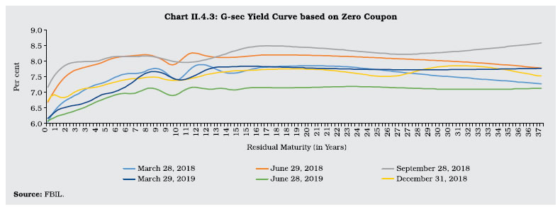 II.4.16 The spread of 5-year AAA-rated corporate bond yield over the corresponding G-sec yield widened by 79 bps, especially in H2, reflecting increased credit risk premia in the aftermath of the IL&FS event and liquidity squeeze faced by some NBFCs. Consequent to the Reserve Bank’s announcement in March 2019 of injecting rupee liquidity through long-term foreign exchange buy/ sell swap auction, both the yield and the spread declined significantly as the move was expected to reduce hedging cost. The average daily turnover in the corporate bond market increased to ₹75.9 billion during 2018-19 from ₹74.6 billion a year ago (Chart II.4.4) II.4.17 Primary corporate bond issuances increased by 7.1 per cent to ₹6,470 billion during 2018-19. While bond issuances declined by 30.3 per cent in H1:2018-19, they increased sharply by 51.4 per cent in H2:2018-19 as softening of corporate bond yields encouraged corporates to resort to increased bond issuances, particularly from December 2018 onwards. Public debt issuances at ₹366.8 billion during 2018-19 registered an increase of more than seven times on a year-on-year (y-o-y) basis. Private placements remained the preferred choice for corporates, accounting for 94.3 per cent of total resources mobilised through bond issuances. Outstanding corporate bonds increased by 11.9 per cent y-o-y to ₹30,672 billion — 16.1 per cent of GDP at end-March 2019. Consequently, FPIs’ utilisation of the approved limit declined to 75.9 per cent from 91.9 per cent at end-March 2018. 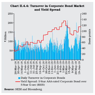 II.4.18 Continuation of softening of G-sec yields and decrease in credit default risk, as reflected in lower credit default swap (CDS) spread, resulted in yield on 5-year AAA-rated corporate bond easing by 14 bps to 7.96 per cent during Q1:2019-20. The yield spread of 5-year AAA-rated corporate bond over 5-year G-sec narrowed by 4 bps. Primary issuances in corporate bond market increased by 43.7 per cent to ₹1,668 billion in Q1:2019-20 as compared with the corresponding period of the preceding year. The average daily turnover in the corporate bond market has increased to ₹86.6 billion in Q1:2019-20 as compared with ₹75.0 billion in Q1:2018-19. 5. Equity Market II.4.19 The equity market registered strong gains in 2018-19, with the benchmark indices touching new peaks interspersed with intermittent corrections. The BSE Sensex and Nifty 50 increased by 17.3 per cent and 14.9 per cent, respectively, on the back of favourable domestic factors and rallies in global markets. The uptrend in the domestic equity market was interrupted by the IL&FS episode but an impressive recovery occurred in H2:2018-19, particularly in the month of March 2019. Positive global cues on account of the Fed’s dovish outlook, favourable developments around the US-China trade talks, the return of FPIs and increasing optimism about the general election outcome helped markets to recover lost ground. The buoyancy in the equity market was largely supported by mutual funds’ purchases, albeit, at a slower pace than a year ago (Chart II.4.5). FPIs were net buyers during the year. 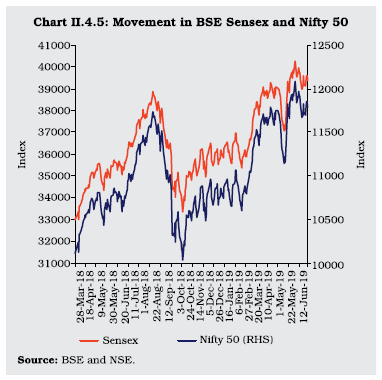 II.4.20 Indian equity indices surged during the first five months of 2018-19, with the BSE Sensex touching a record high of 38897 at close on August 28, 2018. Market sentiment was buoyed by a combination of factors, including lower than expected market borrowing programme of the Centre for H1:2018-19, better than expected corporate earnings performance in Q4:2017-18 and Q1:2018-19, the Government’s approval of capital infusion in public sector banks, reduction in GST rates on several items, better than expected GDP growth in Q1:2018-19 and decline in inflation in July and August. Sporadic bouts of selling were also witnessed during this period on continuing trade related frictions between the US and China, surges in crude oil prices and concerns about potential market contagion from the crisis in Turkey. II.4.21 Market sentiment was severely impacted during September and October 2018 by the IL&FS event and the follow-on liquidity squeeze in the NBFC space, concerns relating to trade war between the US and China, a sharp depreciation of the rupee vis-à-vis the US dollar against the backdrop of higher crude oil prices and widening of India’s current account deficit (CAD) in Q1:2018-19. Markets staged a short-lived turnaround in November 2018, supported by easing of concerns over liquidity tightness, expectations of a breakthrough in the US-China trade relations at the G-20 summit, dovish statements by the US Fed, improvement in India’s ranking in the World Bank’s Ease of Doing Business Index and a sharp appreciation of the rupee against the US dollar. Subsequently, in December 2018, the equity market declined moderately on weaker than expected Q2:2018-19 GDP growth, uncertainty regarding the outcome of state assembly elections and the fourth rate hike in a year by the US Fed. After declining for most part of January 2019, equity markets turned around and the BSE Sensex increased by 1.9 per cent on January 31, 2019 mainly because of the Fed’s decision to hold rates along with the indication that it would adopt a patient approach to further rate hikes. Additionally, positive expectations from the Interim Budget, 2019-20 also contributed to the rally. II.4.22 The equity market commenced on a bullish note in February 2019 on expectations of a dovish monetary policy stance by the Reserve Bank, which was followed by a 25 bps policy repo rate cut coupled with a change in stance to neutral from calibrated tightening. However, sentiment reversed on account of possibility of another partial US Government shutdown due to continuing impasse over funding of the US-Mexico border wall, concerns over the US-China trade talks, India-Pakistan tensions following the terror attack in Kashmir and subsequent escalation of the conflict. However, the Indian equity market rebounded sharply in March 2019, with the BSE Sensex registering gains of 7.8 per cent on the back of positive global cues, easing of cross-border tensions, large investments by FPIs and increasing optimism about general election outcome. II.4.23 The Indian equity market registered modest gains with the BSE Sensex and Nifty 50 increasing by 1.9 per cent and 1.4 per cent, respectively, during Q1:2019-20. The market commenced the year on a positive note, but subdued earning results for Q4:2018-19 coupled with re-escalation of trade tensions dragged markets lower during early May 2019. Subsequently, formation of stable government at the Centre helped markets to resume uptrend with the BSE Sensex recording all-time high of 40268 on June 3, 2019. However, some of the gains were wiped out mainly due to re-emergence of liquidity concerns in NBFC sector especially after delay in servicing of non-convertible debentures by a housing finance company, intensification of trade conflict between the US and China and retaliatory imposition of tariffs on US goods by India with effect from June 16, 2019. II.4.24 Net investment by institutional investors, particularly mutual funds (MFs), during 2018-19 provided support to equity market. FPIs remained net sellers for most part of the year before making heavy investments in February and March 2019. Net purchases by MFs in equities during the year amounted to ₹879 billion, which was sharply lower than purchases of ₹1,418 billion in the previous year. Overall, FPIs made net purchases of ₹97 billion during the year (Chart II.4.6). During Q1:2019-20, MFs made net purchases of ₹68 billion. FPIs made net purchases of ₹216 billion in contrast to net sales of ₹184 billion during Q1:2018-19. Primary Market Resource Mobilisation II.4.25 The primary segment of the equity market exhibited lacklustre activity during 2018-19. Resource mobilisation through public and rights issues was higher in the first five months of 2018-19 on a y-o-y basis; however, it moderated substantially from September 2018 onwards on account of heightened uncertainty and volatile secondary market conditions. Resource mobilisation through initial public offers (IPOs) and rights issues declined by 82.7 per cent to ₹182.4 billion during 2018-19. Companies mobilised a total of ₹160.9 billion through 123 IPO issues, out of which 110 issues amounting to ₹18.4 billion were listed on the small and medium enterprises (SME) platform of the BSE and the NSE. Resource mobilisation through qualified institutional placement (QIP) declined sharply to ₹102.9 billion in 2018-19 from ₹672.4 billion in 2017-18 (Appendix Table 5). II.4.26 Net resource mobilisation by MFs declined by 59.6 per cent to ₹1,097 billion in 2018-19. Resource mobilisation through equity-oriented schemes declined to ₹1,080 billion in 2018-19 from ₹1,711 billion in 2017-18, mainly on account of lower investments by individuals and corporates during 2018-19 than a year ago. Assets under management (AUM) of equity-oriented MFs increased by 19.0 per cent to ₹8,921 billion at end-March 2019 from ₹7,498 billion at end-March 2018. II.4.27 Primary market resource mobilisation through public and rights issues of equity increased significantly by more than eight times (y-o-y) during Q1:2019-20 on account of higher resource mobilisation by telecom companies through rights issues. QIP issues declined by 16.3 per cent during Q1:2019-20. The net resources mobilised by MFs declined significantly by 86.8 per cent during Q1:2019-20 primarily due to decline in net inflows in money market MFs. 6. Foreign Exchange Market II.4.28 In the foreign exchange market, turnover picked up strongly in the inter-bank segment during 2018-19. The Indian rupee remained weak vis-à-vis the US dollar during H1:2018-19 following portfolio rebalancing away from EMEs, including India, strengthening of the US dollar and widening of India’s CAD on account of rising crude oil prices. The rupee continued to weaken till mid-October 2018; however, it started recovering thereafter on account of net purchases by FPIs, a softer monetary policy stance across major central banks, and easing of crude oil prices. The rupee touched an all-time intra-day low of ₹74.49 per US dollar on October 11, 2018 with a depreciation of 12.5 per cent over end-March 2018 level. Overall, the rupee depreciated by 6.0 per cent against the US dollar during 2018-19 (Chart II.4.7). However, on average during 2018-19, the rupee fared better than several other EME currencies. During Q1:2019-20, rupee initially traded with a mild depreciating bias as crude oil prices hovered around their highest levels in 2019. However, rupee witnessed appreciation from mid-May on the back of formation of stable government post general elections, decline in crude oil prices, sustained FPI inflows and a dovish outlook by the US Fed. 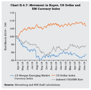 II.4.29 In tandem with movements in the exchange rate of the rupee, the 36-currency nominal/real effective exchange rate (NEER/ REER) recorded persistent depreciation till October 2018, however, it appreciated thereafter. In terms of the 36-currency NEER and REER, the rupee depreciated by 5.6 per cent and 4.8 per cent, respectively, during 2018-19. II.4.30 Forward premia, for most part of the year, remained at levels similar to those in the previous year and were at elevated levels towards the close of the financial year on account of higher forex inflows and year end phenomenon. Turnover in both merchant and the inter-bank segments of the spot and forward market remained largely at levels reached in the previous year, while the swap segment exhibited an increase in activity during the latter part of the year. II.4.31 Going forward, global factors like trade related developments between the US and China and concerns about a slowdown in global growth could weigh upon financial markets. However, strong domestic macroeconomic fundamentals should act as a buffer against volatility. II.5 GOVERNMENT FINANCES II.5.1 In 2018-19, public finances recorded modest deviations from budgetary deficit targets across the general government. For the central government, the overshoot of 0.1 per cent in its gross fiscal deficit (GFD) from the budgeted 3.3 per cent of GDP was mainly due to lower than budgeted collections under income tax and Goods and Services Tax (GST). Consequently, the central government had to take recourse to the Escape Clause as specified under Section 4 (2) of the FRBM Act, 2003. For the states19, there was a deviation of 0.3 per cent of GDP in their consolidated GFD from the budgeted level mainly on account of higher revenue expenditure. II.5.2 There are some noteworthy features of budget outcomes of both centre and states in 2018-19 which mark a break from the past. First, fiscal management vis-à-vis previous year was based on revenue augmentation rather than expenditure rationalisation. Simultaneously, governments committed to enhancing the quality of expenditure by preserving budgeted capital outlays and lowering outlays on the revenue account. Second, a notable development going forward is the establishment of dual targets – in terms of debt and the fiscal deficit – as necessary and sufficient conditions for fiscal prudence, as recommended by the FRBM Review Committee (Chairman: Shri N. K. Singh). The government also committed to bring in some element of counter cyclicality in its fiscal policy by suitably adopting explicit escape and buoyancy clauses. II.5.3 For 2019-20, the centre’s GFD is budgeted at 3.3 per cent of GDP, a consolidation over that achieved in 2018-19 (PA), even with a high revenue expenditure growth. On the other hand, state governments are expecting to firm up their fiscal positions in 2019-20, with their consolidated GFD budgeted at 2.4 per cent of GDP. Accordingly, the general government’s GFD is expected to come down further in 2019-20. II.5.4 Against this backdrop, Sub-sections 2 and 3 present the position of central government finances in 2018-19 and 2019-20, respectively. Sub-sections 4 and 5 depict the developments in state government finances during 2018-19 and 2019-20, respectively. General government finances are discussed in Sub-section 6. 2. Central Government Finances in 2018-19 II.5.5 In 2018-19, the central government’s GFD turned out to be 3.4 per cent of GDP, a deviation of 0.1 per cent of GDP from the target set in the Union Budget, 2018-19. Despite shortfall in income tax and GST collections and additional expenditure for income support scheme under the Pradhan Mantri Kisan Samman Nidhi (PM-KISAN), higher collections under corporation tax, customs and disinvestment receipts, coupled with lower transfer to states helped to compensate for the shortfall while enabling higher capital expenditure. II.5.6 Gross tax collections fell short of the budgeted target in 2018-19 (PA) by ₹1,910 billion largely due to a shortfall in GST collections by ₹1,623 billion and income tax collections by ₹563 billion. On the other hand, corporation tax and customs duty collections surpassed the budget targets by ₹426 billion and ₹54 billion, respectively. Consequently, gross tax collection in 2018-19 (PA) fell to 10.9 per cent of GDP from 11.2 per cent a year ago. In terms of y-o-y growth rates, indirect taxes slowed to 2.9 per cent in 2018-19 from 5.9 per cent in 2017-18, and direct tax growth moderated to 13.5 per cent from 17.9 per cent a year ago. II.5.7 The shortfall in GST collection in 2018-19 can be attributed to the rationalisation of GST rates twice during the year, viz., July 21 and December 22, across sectors and items by the GST council. As a result, the weighted average GST rate came down from 12.2 per cent to 11.6 per cent. On the basis of investigations conducted to detect GST evasion/ violations, it is observed that the amount of tax revenue involved in 3626 evasion/violation cases is estimated at ₹152.8 billion (up to December 2018), of which ₹99.6 billion has been recovered so far. II.5.8 As per the provisional accounts (PA) for 2018-19, dividend transfers and profits from public sector enterprises declined from their level in the previous year, however, surplus transfer from the RBI/banks/financial institutions (FIs) were higher than that in the previous year. Disinvestment proceeds in 2018-19 also exceeded the budgeted target by ₹50 billion. II.5.9 Despite shortfall in tax collection, the government was able to contain GFD to 3.4 per cent of GDP by trimming revenue expenditure by ₹1,333 billion, which includes rollover of food subsidy by ₹674 billion. This allowed the government to maintain the budgeted capital expenditure, which recorded an y-o-y growth of 15.1 per cent in 2018-19 as against a contraction of 7.5 per cent in 2017-18. 3. Central Government Finances in 2019-20 II.5.10 The Union Budget 2019-20 has laid emphasis on boosting the economy via investments mainly in infrastructure, while simultaneously focusing on rural economy, micro, small and medium enterprises (MSMEs) and start-ups. Encouraging research and development and making India healthy, green and clean have also been given importance. Furthermore, the Budget also announced several measures to reform the financial sector that will boost corporate activity, some of which pertain to the Reserve Bank. Higher budgeted revenue expenditure is expected to be met by higher receipts, both direct and indirect, as well as a moderation in capital expenditure. In ensuing years, the government intends to improve expenditure efficiency and improve tax collections to ensure alignment with the fiscal deficit path as prescribed under the FRBM Act. II.5.11 The GFD for 2019-20 is budgeted at 3.3 per cent of GDP as against the projected GFD of 3.1 per cent in the Medium Term Fiscal Policy (MTFP) 2018-19 (Table II.5.1). This fiscal consolidation is expected to be met by higher budgeted direct and indirect tax collection, non-tax revenue and disinvestment receipts. Underpinning the projections of gross tax revenue is an implicit tax buoyancy of 1.67 in 2019-20 (BE), which is much higher than the realised buoyancy of 0.75 in 2018-19 (PA). The budgeted buoyancy of 1.86 for personal income tax for 2019-20 is higher than 1.17 in 2018-19 (PA), which is also the average during 2008-18. Receipts from non-tax revenues are budgeted to increase by 27.2 per cent in 2019-20, with major contributions from dividends and profits of PSUs. Encouraged by the disinvestment outcomes in 2018-19 (PA), the target for disinvestment has been set at ₹1,050 billion in 2019-20 (BE). II.5.12 Total expenditure is budgeted to grow at 20.5 per cent in 2019-20 as against 7.9 per cent in 2018-19 (PA) (Chart II.5.1), attributable to a sharp increase in growth of revenue expenditure from 6.9 per cent in 2018-19 (PA) to 21.9 per cent in 2019-20 (BE). Expenditure on major subsidies, viz., food, fuel and fertilizers, is budgeted to rise to 1.4 per cent of GDP in 2019-20 from 1.0 per cent in 2018-19 (PA). | Table II.5.1: Central Government’s Fiscal Performance** | | (Per cent to GDP) | | Item | 2004-08 | 2008-10 | 2010-15 | 2013-14 | 2014-15 | 2015-16 | 2016-17 | 2017-18 | 2018-19 (RE) | 2018-19 (PA) | 2019-20 (BE) | | 1 | 2 | 3 | 4 | 5 | 6 | 7 | 8 | 9 | 10 | 11 | 12 | | Non Debt Receipts | 11.0 | 9.7 | 9.5 | 9.4 | 9.2 | 9.1 | 9.4 | 9.1 | 9.6 | 8.8 | 9.9 | | Tax Revenue (Gross) (a+b) | 10.7 | 10.4 | 10.2 | 10.1 | 10.0 | 10.6 | 11.2 | 11.2 | 11.8 | 10.9 | 11.7 | | Tax Revenue (Net)* | 7.9 | 7.6 | 7.3 | 7.3 | 7.2 | 6.9 | 7.2 | 7.3 | 7.8 | 6.9 | 7.8 | | a) Direct Tax | 5.1 | 6.0 | 5.7 | 5.7 | 5.6 | 5.4 | 5.5 | 5.9 | 6.3 | 6.0 | 6.3 | | b) Indirect Tax | 5.6 | 4.4 | 4.5 | 4.4 | 4.4 | 5.2 | 5.6 | 5.3 | 5.5 | 5.0 | 5.3 | | Non-tax Revenue | 2.2 | 1.8 | 1.8 | 1.8 | 1.6 | 1.8 | 1.8 | 1.1 | 1.3 | 1.3 | 1.5 | | Non Debt Capital Receipts | 0.9 | 0.3 | 0.4 | 0.4 | 0.4 | 0.5 | 0.4 | 0.7 | 0.5 | 0.5 | 0.6 | | Total Expenditure | 14.5 | 16.1 | 14.4 | 13.9 | 13.3 | 13.0 | 12.9 | 12.5 | 12.9 | 12.2 | 13.2 | | Revenue Expenditure | 12.1 | 14.4 | 12.6 | 12.2 | 11.8 | 11.2 | 11.0 | 11.0 | 11.3 | 10.6 | 11.6 | | Capital Expenditure | 2.4 | 1.7 | 1.8 | 1.7 | 1.6 | 1.8 | 1.9 | 1.5 | 1.7 | 1.6 | 1.6 | | Revenue Deficit | 2.0 | 5.0 | 3.5 | 3.2 | 2.9 | 2.5 | 2.1 | 2.6 | 2.2 | 2.3 | 2.3 | | Gross Fiscal Deficit | 3.5 | 6.3 | 4.9 | 4.5 | 4.1 | 3.9 | 3.5 | 3.5 | 3.3 | 3.4 | 3.3 | BE: Budget Estimates;
RE: Revised Estimates;
PA: Provisional Accounts.
* Net tax revenue represents gross tax revenue net of devolution to state governments.
** GDP figures used in this table are on 2011-12 base, which are the latest available estimates. Going by the principle of using latest available GDP data for any year, GDP used for 2018-19 (RE) is the latest available Provisional Estimate (released on May 31, 2019). In view of this, the fiscal indicators as per cent to GDP given in this Table may at times marginally vary from those reported in the Union Budget Documents
Source: Union Budget Documents. | 4. State Finances in 2018-19 II.5.13 As per the information available for 27 state governments, the consolidated fiscal position of states deteriorated in 2018-19 (RE) vis-à-vis their budget estimates (Chart II.5.2), with their GFD at 2.7 per cent vis-à-vis 2.4 per cent in BE. The revenue account turned into deficit in 2018-19 (RE) from surplus budgeted for the same year because of continued upward pressure emanating from farm loan waivers, income support schemes and hike in minimum support prices by certain states20. This erosion was partly compensated by higher revenue receipts in the form of grants, particularly compensation cess.
5. State Finances in 2019-20 II.5.14 State governments are expecting to consolidate their fiscal position in 2019-20. The combined GFD of states is budgeted at 2.4 per cent, with consolidation mainly through expenditure compression—both revenue and capital, thus, compromising the quality of fiscal consolidation. Notwithstanding the fiscal consolidation, risks continue to persist with 11 states budgeting their fiscal deficits higher than the 3.0 per cent FRBM threshold21. 6. General Government Finances22 II.5.15 The general government GFD has moderated from 6.9 per cent of GDP in 2016-17 to 5.9 per cent in 2018-19. For the first time from 2017-18, the combined GFD has been ruling below 6.0 per cent after remaining above 6 per cent between 2008-09 to 2016-17. Both centre and states have made concerted efforts for fiscal consolidation during the period despite revenue pressures on account of implementation of GST. While centre has done so with the help of extra budgetary resources, the states, on the other hand, have cut capital expenditure so as to bring down the combined GFD-GDP ratio. The general government GFD is budgeted to be 5.7 per cent of GDP in 2019-20 as against 5.9 per cent in the revised estimates for 2018-19 (Appendix Tables 6 & 7). Outstanding liabilities of the general government are budgeted to decline to 67.7 per cent of GDP at end-March 2020 from 68.1 per cent at end-March 2019 (RE). This is in line with the aim of attaining a central government debt to GDP ratio of 40 per cent and a general government debt to GDP ratio of 60 per cent by 2024-25. Though the current debt levels are above the FRBM target, the debt servicing capacity of the general government has improved in 2018-19 with the interest payments as per cent to revenue receipts exhibiting a decline. II.5.16 To sum up, the Union Budget, 2018-19 had to undertake a recalibration in the path of fiscal consolidation in view of the implementation of a major structural reform embodied in the GST in 2017-18. Nonetheless, it is envisaged that the GFD-GDP target of 3.0 per cent will be achieved by 2020-21 in pursuance of the FRBM Act. Consequently, the Union Budget for 2019-20 has pegged the central government’s GFD-GDP ratio at 3.3 per cent as an intermediate step towards converging to a GFD-GDP ratio of 3.0 per cent. Analogously, states have also committed to improve their finances in 2019-20 to contain their combined GFD to 2.4 per cent of GDP. Accordingly, the central government and general government debt are slated to be brought down to 40 per cent and 60 per cent of GDP, respectively, by 2024-25. Going forward, broadening the tax base through structural reforms, coupled with enhanced GST compliance and increased tax efficiency, could help both the centre and states in managing these pressures and in getting back to the path of fiscal consolidation over the medium-term. II.6 EXTERNAL SECTOR II.6.1 Over the greater part of the year 2018-19, financial conditions tightened as global financial markets re-priced risks on a combination of global spillovers alluded to earlier, country-specific factors, spark off scrambles for safe havens, and sell-offs and capital outflows across emerging market economies (EMEs). Downside risks became accentuated as several major economies reported deceleration in growth. The loss of momentum progressively broadened and global growth slowed in 2018 after registering a six year high in 2017. Growth in world trade volume moderated to 3.7 per cent in 2018 from 5.5 per cent a year ago, continuing to trail global output (Chart II.6.1), with the income elasticity23 of world trade declining to 1.0 in 2018 from 1.4 in the previous year. Owing to tight supply conditions and sustained economic activity in H1:2018, global oil inventories fell rapidly and pushed up price to over US$ 80 per barrel in early October ahead of US sanctions against Iran that took effect in November 2018. However, waivers granted by the US to major oil importers from Iran and higher production in Saudi Arabia and Russia eased oil prices in the subsequent period and augured well for oil importing countries like India. 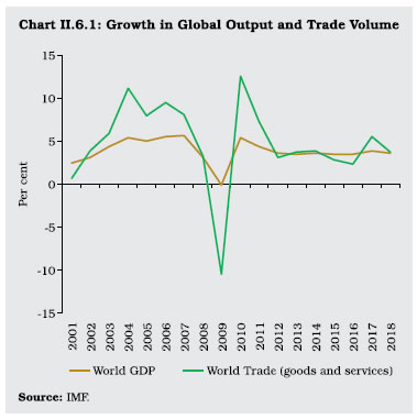 II.6.2 These tumultuous global developments impinged on India’s external sector as manifested in subdued export growth, elevated imports of petroleum products and a higher current account deficit (CAD) than a year ago, notwithstanding resilient services exports and remittances. In conjunction with portfolio outflows, this necessitated a drawdown of foreign exchange reserves. Global risks ebbed in Q4:2018-19 and improved market sentiment rejuvenated the appetite for risk, bringing back portfolio flows to EMEs, including India, and this allowed a recouping of international reserves. II.6.3 Against this backdrop, the following sub-section discusses developments in merchandise exports and imports. Sub-section 3 analyses the behaviour of invisibles and the widening of the CAD. Sub-section 4 dwells on net capital flows and movements in reserves. External vulnerability indicators are evaluated in sub-section 5, followed by concluding observations. 2. Merchandise Trade II.6.4 In an environment of slowing global demand, India’s merchandise export growth decelerated to 8.7 per cent in US dollar terms in 2018-19 from 10.0 per cent in the previous year. Volume growth moderated to 4.3 per cent from 5.6 per cent last year and unit value realisation growth remained at 4.4 per cent; same as in the previous year. II.6.5 Over sixty per cent of the export basket either decelerated or declined during the year. The drag emanated from sectors such as engineering goods, gems and jewellery, marine products and readymade garments. Within engineering goods, exports of iron and steel, and aluminium were affected by higher tariffs imposed by the US in May 2018, while domestic supply constraints led to a sharp decline in copper exports (Chart II.6.2). Iron and steel exports had to also contend with heightened competition in third-country markets. (Chart II.6.3 and Box II.6.1). 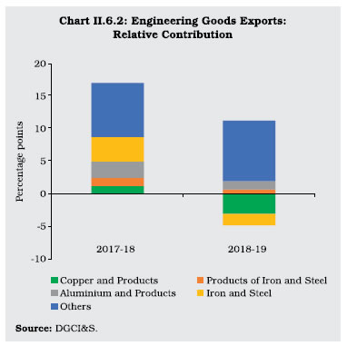 II.6.6 Among the major export items, gems and jewellery exports declined during 2018-19, largely driven by the fall in gold exports as the ban on export of gold articles over 22 carat purity took hold. The revelations of fraud in some domestic banks and subsequent ban on Letter of Undertakings had a transient impact. Unusually hostile weather conditions, low prices and breakout of multiple diseases adversely affected domestic production and exports of marine products, particularly shrimps. In addition, the seafood import monitoring programme in the US led to a contraction in Indian shrimp exports to the US by 6.6 per cent during 2018-19. The decline in exports of readymade garments was conditioned by issues related to delays in reversal of input tax credit, particularly on man-made fabrics, and the imposition of a value added tax (VAT) by the UAE, which is the second largest export destination for Indian readymade garments. Despite a moderation in export growth, India was able to maintain its share in global exports at 1.7 per cent in 2018 and the exports at US$ 330.1 billion reached their highest ever level (the previous high of US$ 314.4 billion in 2013-14). The sectors which witnessed robust export growth in 2018-19 included organic chemicals and electronic goods. 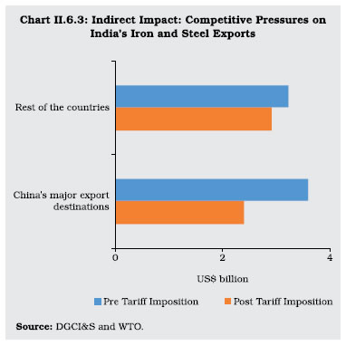 II.6.7 Merchandise imports which had been growing in double digits during H1:2018-19 slowed down during H2 and grew at 10.6 per cent for the year as a whole during 2018-19, a marked deceleration from 20.9 per cent growth in the previous year (Table II.6.1). The moderation in imports occurred despite petroleum imports rising by 29.7 per cent on the back of a 23.5 per cent (y-o-y) increase in international crude oil prices and a modest increase in import volume. With major oil producers (OPEC and major non-OPEC) recommitting to production cuts of about 1.8 million barrels per day through 2017 and 2018 and with improved compliance, crude oil prices rose sharply from US$ 54.5 per barrel in September 2017 to US$ 80.1 per barrel in October 2018. However, with record US shale oil production and OPEC over-production during the latter part of 2018 combined with a slowdown in global demand, oil prices fell after October 2018 till February 2019 but firmed up in March-April 2019. In addition, a pick-up in demand combined with supply disruptions due to the Iran sanctions and lower production in Venezuela added pressure to oil prices. Box II.6.1
India’s Third-market Export Competition in Manufacturing Goods International competitiveness is influenced, inter alia, by price/cost differentials between home and trading partner countries and in third-country markets as well. Effective exchange rates (EER), both nominal and real, are widely used indicators of international price and cost competitiveness. Double weights schemes are employed to take into account both direct and third-market export competition (Turner and Van’t dack, 1993). Algebraically, export weight (wj) to be assigned to trading partner economy j in EER basket of i can be expressed as: The first term on the right-hand side of above equation represents the direct export competition faced by economy i’s exports in trading partner j’s market. The second term in the equation measures the third-market competition between exports of i and j in r. When r is an important market for exports of i and j, economy j should be assigned a higher weight in i’s EER basket. For India, the largest third-market competitor is China (apparel, textile fabrics, footwear and musical instruments), followed by the euro area which is the largest export competitor of India in manufactured goods (Chart 1).
| Table 1: India’s Top 10 Competitive Third-markets | | Third-market | Weight (Per cent) | Top 3 Competitors | | 1 | 2 | 3 | | 1. UAE | 16.4 | China, Euro Area, and US | | 2. US | 15.8 | China, Euro Area, and Mexico | | 3. Euro Area | 12.5 | China, US, and UK | | 4. UK | 7.7 | Euro Area, China, and US | | 5. Hong Kong | 6.3 | China, Singapore, and Taiwan | | 6. Singapore | 3.4 | China, Euro Area, and Mexico | | 7. Bangladesh | 2.6 | China, Euro Area, and Singapore | | 8. Mexico | 2.4 | US, China, and Euro Area | | 9. China | 2.2 | Hong Kong, Euro Area, and Korea | | 10. Saudi Arabia | 2.2 | Euro Area, China, and US | | Total | 71.4 | | Note: Weights are based on average for 2014-18.
Source: UNCTAD and RBI staff calculations. | The UAE is the largest third-market for India’s manufacturing exports, in which highest competition is faced from China, the euro area, and the US. Other major third-markets include the US, the euro area, the UK, and Hong Kong, which together account for 59 per cent of third-market competition for India (Table 1). The double-weighting methodology has certain limitations. It is based on the assumption of trade of one type of good with constant elasticity of substitution, which is not realised in real life, given the high degree of international product differentiation and vertical specialisation. Consequently, the changes in currencies of trading partners may not have the same impact on relative demand or prices for given weights (Klau and Fung, 2006). Nevertheless, EERs based on double-weighting are more representative of international competitiveness than single-weighting schemes. References: 1. Klau, M. and S.S. Fung (2006), ‘The New BIS Effective Exchange Rate Indices’, BIS Quarterly Review, Bank for International Settlements, March. 2. Turner, P. and J. Van‘t dack (1993), ‘Measuring International Price and Cost Competitiveness’, BIS Economic Papers, Bank for International Settlements, No. 39, November. |
Table II.6.1: Growth in Merchandise Trade
(y-o-y, per cent) | | | 2017-18 | 2018-19 | | 1 | 2 | 3 | | Exports | | | | Q1 | 8.5 | 15.3 | | Q2 | 12.3 | 9.7 | | Q3 | 14.1 | 4.5 | | Q4 | 5.5 | 6.7 | | Annual | 10.0 | 8.7 | | Imports | | | | Q1 | 34.5 | 12.7 | | Q2 | 19.7 | 22.8 | | Q3 | 17.9 | 8.1 | | Q4 | 14.0 | 0.3 | | Annual | 20.9 | 10.6 | | Source: DGCI&S. | II.6.8 Merchandise import growth was also pulled down by a decline in gold imports brought about by a fall in international gold prices in spite of somewhat higher volume of imports than a year ago. Growth in non-oil non-gold imports slowed considerably during 2018-19, indicative of a weakening domestic demand (Chart II.6.4). II.6.9 Within non-oil non-gold imports, contraction in imports of vegetable oils, pulses, and pearls and precious stones and pronounced slowdown in electronic goods imports were the main drags.  II.6.10 Tariff escalations and stricter rules of origin policies triggered a decline of 15.0 per cent in vegetable oil imports during 2018-1924. While imports of all components of pearls and precious stones shrank, the import of pearls from Hong Kong crashed from exceptionally high imports of US$ 2.1 billion during 2017-18 to US$ 9.8 million during 2018-19. Imports of diamonds were adversely affected by the hike in import tariffs in September 2018. The growth in electronic goods imports, which account for 10.8 per cent of the import basket and are the second largest item in India’s import basket, slowed down from 22.9 per cent in 2017-18 to 7.6 per cent during 2018-19. Telecom instruments, comprising mobile phones and parts of mobile phones among other components, recorded a decline during 2018-19 (Chart II.6.5). This coincided with an increase in the domestic production of mobile phones, the impetus to which was provided by the government’s Phased Manufacturing Programme, announced in the Union Budget 2015-16 (Box II.6.2).  II.6.11 These developments resulted in a widening of the trade deficit to US$ 184.0 billion in 2018-19 (6.8 per cent of GDP) from US$ 161.3 billion (6.1 per cent of GDP) in the previous year. Terms of trade losses augmented the trade deficit by US$ 7.1 billion. On a bilateral basis, a notable development is the reduction in India’s trade deficit with China and Indonesia, even as India’s trade surplus with the US shrank as India’s imports from the US grew much faster than India’s exports to the US (Chart II.6.6). Petroleum products and diamonds accounted for most of the increase in India’s imports from the US during 2018-19. 3. Invisibles II.6.12 Net receipts from invisibles, comprising services, income and transfers, recorded double-digit growth during 2018-19. Net invisibles could, however, finance only 68 per cent of the merchandise trade deficit as compared with 70 per cent in the previous year. Box II.6.2
India: Emerging Electronics Exporter The electronics industry is among the largest and fastest growing manufacturing industries globally, with production estimated at US$ 2.9 trillion in 201825. Concomitantly, it has emerged as a significant engine of cross-border trade. In India, domestic production has been able to meet only about one-third of domestic demand, leaving a substantial portion to be met by imports. Currently, India’s electronic goods imports account for 2.0 per cent of world’s electronic imports. India’s demand for electronic goods is estimated to reach US$ 400 billion by 2025. Consequently, the trade balance in this segment has deteriorated during the last two decades to a deficit of US$ 48.0 billion in 2018-19. Cognizant of these challenges, the government has taken several measures to improve the competitiveness of Indian electronics manufacturers through tariff structure rationalisation, infrastructure upgradation, procedure simplification and provision of incentives. Electronics manufacturing is an important constituent of the ‘Make in India’ and ‘Digital India’ programmes. The Union Budget 2015-16 introduced the Phased Manufacturing Programme (PMP) for mobile handsets and related sub-assemblies/ components manufacturing, involving a countervailing duty on mobile phone imports, a differential excise duty structure for domestic mobile phone manufacturing and exemption of parts/components/accessories of mobile phones from basic customs duty to encourage domestic manufacturing of mobile phones (assembly, programming, testing and packaging). In addition, the Electronic Development Fund was created in February 2016 to provide risk capital to firms developing new technologies in the sphere of electronics and information technology (MeitY, 2018). With Make in India, mobile phone handsets and components manufacturing have emerged as a flagship sector26. Domestic mobile phone production has enabled a decline of mobile phone imports (Table 1). | Table 1: Production of Electronic Goods in India | | (US$ billion) | | Item | 2014-15 | 2015-16 | 2016-17 | 2017-18 | 2018-19 | | 1 | 2 | 3 | 4 | 5 | 6 | | Consumer Electronics | 9.1 | 8.5 | 9.7 | 11.4 | 11.0 | | Industrial Electronics | 6.4 | 6.9 | 9.3 | 10.7 | 11.6 | | Computer Hardware | 3.1 | 3.0 | 3.0 | 3.3 | 3.0 | | Mobile Phones | 3.1 | 8.2 | 13.4 | 20.5 | 24.3 | | Strategic Electronics | 2.6 | 2.8 | 3.1 | 3.7 | 4.0 | | Electronics Components | 6.5 | 6.9 | 7.8 | 9.2 | 9.7 | | Light Emitting Diodes | 0.4 | 0.8 | 1.1 | 1.5 | 1.9 | | Total | 31.2 | 37.1 | 47.4 | 60.3 | 65.5 | Note: Annual average USD-INR exchange rate is used to express in US dollar terms.
Source: Annual Report 2018-19, Ministry of Electronics & Information Technology (MeitY), Government of India. | Econometric evidence indicates the presence of a structural break in the imports of smartphones in September 2015, followed by a consistent decline (Table 2) (Misra and Shankar, 2019). Domestic production is negatively correlated with the imports of mobile phones but positively correlated with imports of parts of mobile phones (Table 3). This is bolstered by the finding that domestic production is ‘granger caused’ by increased imports of mobile phone parts (Table 4). Outward shipments of smartphones have increased from US$ 0.2 billion during 2017-18 to US$ 1.6 billion during 2018-19. The UAE, Russia, South Africa and China are emerging as important export destinations. | Table 2: Testing for Structural Breaks in Smartphone Imports Quandt-Andrew’s Unknown Breakpoint Test | | Dependent Variable: SMARTYOY | Method: Least Squares with Breaks | | Null Hypothesis: No breakpoints within 15 per cent trimmed data | | Break type: Bai-Perron tests of L+1 vs. L sequentially determined breaks | | Sample (adjusted): 2012M04 2018M12 | Test Sample: 2013M05 2017M12 | | Number of breaks compared: 56 | Break: 2015M09 | | Statistic | Value | Prob. | Variable | Coef. | Std. Error | Prob. | | Maximum LR F-statistic (2015M09) | 125.2 | 0.00 | 2012M04 - 2015M08 (41 obs) | 10.36 | 2.83 | 0.00 | | Exp LR F-statistic | 58.8 | 0.00 | 2015M09 - 2018M12 (40 obs) | -45.16 | 6.40 | 0.00 | | Ave LR F-statistic | 53.3 | 0.00 | Durbin-Watson statistic | 1.35 | | | | | | | F-statistic | 125.18 | | | | | | | Prob (F-statistic) | 0.00 | | | Notes: 1. SMARTYOY refers to month-wise year-on-year change in volume of smartphone imports.
2. Probabilities calculated using Hansen’s (1997) method. |
| Table 3: Correlations | | | Mobile Phone Imports (Volume) | Parts of Mobile Phone Imports (Volume) | IIP Mobile Phone | | Mobile Phone Imports (Volume) | 1.00 | - | - | | Parts of Mobile Phone Imports (Volume) | -0.64 | 1.00 | - | | IIP Mobile Phone | -0.72 | 0.65 | 1.00 | Sample period: April 2012 – December 2018.
Note: All correlations are significant at 1 per cent level. |
| Table 4: Pairwise Granger Causality Test Result | | Null Hypothesis: | F-Statistic | Prob. | | Mobile phone parts (y-o-y) does not Granger Cause IIP mobile phones (y-o-y) | 4.57 | 0.02 | | IIP mobile phones (y-o-y) does not Granger Cause mobile phone parts (y-o-y) | 0.60 | 0.55 | Observations: 44 (April 2015 – December 2018)
No of lags: 2 | References: 1. MeitY (2018), ‘Electronics and Information Technology’, Annual Report 2017-18, Government of India. 2. Misra, R., and A. Shankar (2019), ‘India Connected: Transforming India’s Import Profile’, RBI Bulletin, April. |
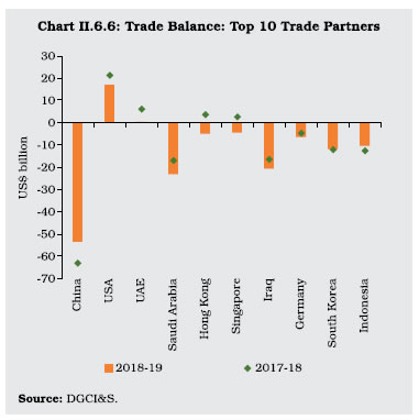 II.6.13 Among the major categories of services, export of travel services declined significantly, owing to moderate growth in foreign tourist arrivals during 2018-19, especially from higher per capita income countries such as the US (accounting for 14 per cent of the total) and the UK (accounting for 9 per cent of the total). By contrast, travel payments by outbound Indian tourists increased significantly, resulting in a decline in net travel receipts by 24 per cent. II.6.14 India’s software exports demonstrated resilience, surviving difficult global market conditions during the year. India remained the top exporter of telecommunications, computer and information services in the world with share of around 10 per cent. During 2018-19, Indian software exports grew by around 7.6 per cent on a y-o-y basis on the back of strong performance of banking, financial services and insurance (BFSI) verticals. India’s software exports may face a challenging business environment with global economic activity and global IT spending forecast to grow at a modest pace in 2019 and 2020. Apart from these uncertainties, a higher rejection rate among Indian IT companies in getting H-1B visas may increase the cost of delivering on-site services and affect their profit margins. Geographical and product diversification would help in mitigating the associated risks. Furthermore, focusing on larger digital deals, reskilling the local talent in export markets and moving up in the value chain may help IT companies build resilience in their export earnings. II.6.15 Inbound remittances by Indians employed overseas rebounded during 2018-19. In 2018, India retained its top position followed by China, Mexico, the Philippines and Egypt27. With over 50 per cent of remittances from Gulf countries, improved income conditions owing to the sharp increase in international crude oil prices augured well for remittances flows in 2018-19. Furthermore, remittances to Kerala also got a fillip in the aftermath of floods in August 2018 as highlighted by the World Bank (April 2019). However, the World Bank projects global remittances to grow at a slower pace in 2019 and 2020 relative to 2018. In the case of India, a 13 per cent fall in 2018 in the number of low-skilled emigrants seeking mandatory clearance for emigration may impact the outlook for in-bound remittances. II.6.16 The net outgo in the form of payments of interest and dividend for servicing the stock of foreign liabilities increased marginally to US$ 28.9 billion in 2018-19 from US$ 28.7 billion a year ago. Debt liabilities in the form of interest payments, which includes payment of interest by foreign direct investment (FDI) enterprises to their parent companies abroad, foreign portfolio investment (FPI) debt holdings, external commercial borrowings (ECBs), trade credits, bank overseas borrowings, non-resident deposits, coupled with non-debt liabilities in the form of dividend pay-outs on investment in equity and investment fund shares accounted for around 70 per cent of total investment income outgoes in 2018-19. A predominant part of dividend payments is, however, deployed back by domestic FDI companies. II.6.17 The CAD widened to 2.1 per cent of GDP from 1.8 per cent a year ago, primarily on the back of the higher trade deficit (Chart II.6.7). While the erosion in net terms of trade (ToT) caused by higher commodity prices (e.g., crude oil, coal and fertilisers) added 0.5 percentage points of GDP to the incremental CAD during 2018-19, higher import volumes contributed another 0.1 percentage points (Chart II.6.8).
4. External Financing II.6.18 Net capital flows were not sufficient to finance the higher CAD, given net outflow of FPI (Chart II.6.9). This led to a depletion of foreign exchange reserves after six consecutive years of accretion on a BoP basis. II.6.19 Within capital flows, FDI remained predominant as in the preceding year (Table II.6.2), though it could finance only 53.6 per cent of the CAD in 2018-19 as compared with 62.2 per cent a year ago. In response to the improvement in the domestic business environment, resilient growth prospects and low inflation, India has attracted a considerable amount of FDI in recent years. With further rationalisation of domestic business procedures (e.g., introduction of the GST) and focus on automatic route with minimal intervention, India gained 23 notches in terms of the World Bank’s ease of doing business index (2019)28 and was ranked 77th among 190 countries. Higher FDI flows went to sectors such as manufacturing, financial services, retail and wholesale trade and computer services. Singapore and Mauritius remained the major source countries, followed by the USA, Japan and the Netherlands. India’s amended double taxation avoidance agreement (DTAA) with Mauritius for the prevention of taxes on income and capital gains led to a decline of 51 per cent in FDI routed through Mauritius in 2018-19. Despite similar changes in the DTAA treaty, Singapore remained the most preferred route for foreign companies to invest in India (Chart II.6.10 and Appendix Table 9). 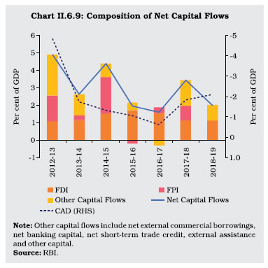
| Table II.6.2: Foreign Direct Investment Inflows | | (US$ billion) | | Item | 2016-17 | 2017-18 | 2018-19 | | 1 | 2 | 3 | 4 | | 1 Net FDI (1.1 - 1.2) | 35.6 | 30.3 | 30.7 | | 1.1 Net Inward FDI (1.1.1 - 1.1.2) | 42.2 | 39.4 | 43.3 | | 1.1.1 Gross Inflows | 60.2 | 61.0 | 62.0 | | 1.1.2 Repatriation/Disinvestment | 18.0 | 21.5 | 18.7 | | 1.2 Net Outward FDI | 6.6 | 9.1 | 12.6 | | Source: RBI. | II.6.20 India’s FDI performance is also noteworthy in the context of global FDI which fell by 13 per cent in 2018 to an estimated US$ 1.3 trillion from US$ 1.5 trillion in 2017 (UNCTAD, 2019). This was mainly due to large repatriations of retained earnings by the US-based multinational enterprises in the aftermath of corporate tax reforms in the preceding year. India was among the few major EMEs that received higher inward FDI during the period. II.6.21 Domestic firms continued to expand their overseas business operations by enhancing direct investment stakes abroad. Outward FDI was mainly in the form of equity and loans to subsidiaries/affiliated enterprises by resident firms, 66 per cent went to financial, insurance and business services, and manufacturing. Two-thirds of the outward FDI was directed to the USA, Singapore, the UK, the Netherlands and the UAE. II.6.22 As regards FPI flows, there was net sale of US$ 2.2 billion in 2018-19 as against a net purchase of US$ 22.2 billion in 2017-18. This essentially reflected global portfolio rebalancing as investors turned away from EMEs and shifted to safe haven assets during April-December 2018. In Q4:2018-19, however, FPIs responded to the ebbing of global risks and made net purchases of about US$ 11.5 billion in the domestic capital market, partly recouping the net sales of US$ 13.7 billion in the preceding three quarters (Chart II.6.11). Although investment limits for FPIs in both government securities and corporate bonds were enhanced during the year, the utilisation of these limits fell in both segments. The composition of assets under custody as at end-March 2019 shows that US-based FPIs accounted for one-third of total outstanding FPI holdings while the share of Mauritius-based FPIs declined in the aftermath of India’s amended DTAA protocol and stiffer KYC norms for FPIs from ‘high risk’ jurisdictions (Chart II.6.12). Various policy measures were undertaken to expand investment opportunities for FPIs, which, inter alia, included (i) relaxing the minimum residual maturity requirement in government securities (including in Treasury Bills), subject to certain conditions; and (ii) permitting FPIs to invest in corporate bonds with minimum residual maturity of above one year instead of three years. Furthermore, in order to boost long-term FPI investment, the Reserve Bank introduced a ‘Voluntary Retention Route’ scheme under which investments by FPIs in the debt market are not subject to macroprudential and other regulatory norms, provided they voluntarily commit to retain a required minimum percentage of their investments in India for a minimum period of three years. 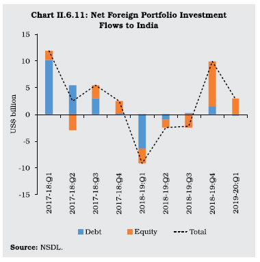
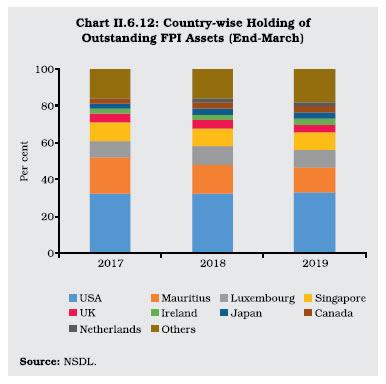 II.6.23 Among other forms of financial flows, ECBs29 to India recorded net inflows of US$ 9.8 billion in 2018-19 as against an outflow of US$ 0.8 billion a year ago. Various measures were undertaken to rationalise the extant ECB policy framework which included (i) merging of Tracks I and II into foreign currency denominated ECBs and rupee denominated ECBs; (ii) allowing a borrowing limit of US$ 750 million a year under the automatic route; (iii) expansion of the list of eligible borrowers to include all entities eligible to receive FDI, registered entities engaged in micro-finance activities, registered societies/trusts/ cooperatives and non-government organisations; (iv) reduction of tenure for exemption of mandatory hedging for eligible borrowers from 10 years to 5 years; (v) easing of end-use restrictions; (vi) reduction in the minimum average maturity requirement for borrowings in the infrastructure sector to three years; and (vii) permitting public sector oil marketing companies to raise ECBs for working capital purposes. Besides, a rule-based dynamic limit was introduced by capping the outstanding ECBs at 6.5 per cent of GDP at current market prices. The top five sectors that accounted for more than 80 per cent of the value of ECB agreements were financial services, petroleum, iron and steel, telecommunication, and power transmission and distribution. Of the total ECB agreement amount (other than rupee denominated bonds/loans), 45.6 per cent was intended to be hedged during 2018-19 as compared with 32.5 per cent a year ago. While 21 per cent of total ECB agreement amount was intended to be raised through rupee denominated loans/bonds (RDBs), actual inflows of RDBs were US$ 0.5 billion as compared with US$ 2.6 billion a year ago. II.6.24 In the aftermath of the discontinuation of Letters of Undertaking (LoUs)/Letters of Comfort (LoCs) in March 2018, importers’ recourse to buyers’ credit declined sharply, partly substituted by an increase in suppliers’ credit. Trade credit was primarily availed by domestic companies to finance imports of crude oil, coal and copper which together accounted for around 45 per cent of the total short-term trade credit raised during the year. In order to ease trade financing conditions, the trade credit limit under the automatic route was raised to US$ 150 million or equivalent for import transactions of oil/gas refining and marketing, airline and shipping companies, and to US$ 50 million or equivalent per import transaction for other sectors, in March 2019. The spread over LIBOR for all-in-cost ceiling was reduced to 250 bps from 350 bps earlier. II.6.25 Non-resident deposit flows recorded an increase of 7.4 per cent in 2018-19 on the back of increased inflows under Non-Resident (External) Rupee accounts (NRE) and Non-Resident Ordinary (NRO) accounts. Deposits under the NRE scheme contributed 70 per cent of net flows during the year. The rupee’s depreciation and improved income conditions in home countries of non-residents boosted these flows (Table II.6.3). 5. Vulnerability Indicators II.6.26 At end-March 2019, India’s external debt increased by US$ 13.7 billion (i.e., 2.6 per cent) from its level at end-March 2018, primarily on account of an increase in short-term debt, commercial borrowings and non-resident deposits. The appreciation of the US dollar vis-à-vis Indian rupee and other major currencies resulted in a valuation gain of US$ 16.7 billion. Excluding the valuation effect, the increase in external debt would have been US$ 30.4 billion instead of US$ 13.7 billion at end-March 2019 over end-March 2018. Commercial borrowings remained the largest component of external debt with a share of 38.0 per cent, followed by non-resident deposits (24.0 per cent) and short-term trade credit (18.9 per cent). As a ratio to GDP, external debt declined from 20.1 per cent at end-March 2018 to 19.7 per cent at end-March 2019. Notwithstanding this favourable development, some external vulnerability indicators worsened during the year. The share of short-term debt (on both original and residual maturity basis) in total external debt increased, while the reserves cover of imports and short-term debt (on both original and residual maturity basis) declined partly reflecting depletion of reserves during the year. Consequently, India’s net international investment position (NIIP) deteriorated by US$ 17.9 billion. Taken together, however, external sector indicators at end-March 2019 were stronger than their levels during the pre-taper talk period (Table II.6.4, and Appendix Table 1 and 8). | Table II.6.3: Flows under Non-Resident Deposit Accounts | | (US$ billion) | | | 2016-17 | 2017-18 | 2018-19 | | 1 | 2 | 3 | 4 | | 1. Non-Resident External (Rupee) Account | 9.8 | 7.1 | 7.3 | | 2. Non-Resident Ordinary Account | 2.2 | 1.5 | 1.9 | | 3. Foreign Currency Non-Resident (B) Account | -24.3 | 1.0 | 1.1 | | Non-Resident Deposits (1+2+3) | -12.4 | 9.7 | 10.4 | | Source: RBI. |
| Table II.6.4: External Vulnerability Indicators (End-March) | | (Per cent, unless indicated otherwise) | | Indicator | 2013 | 2017 | 2018 | 2019 | | 1 | 2 | 3 | 4 | 5 | | 1. External Debt to GDP ratio | 22.4 | 19.9 | 20.1 | 19.7 | | 2. Ratio of Short-term Debt (original maturity) to Total Debt | 23.6 | 18.7 | 19.3 | 20.0 | | 3. Ratio of Short-term Debt (residual maturity) to Total Debt | 42.1 | 41.6 | 42.0 | 43.4 | | 4. Ratio of Concessional Debt to Total Debt | 11.1 | 9.4 | 9.1 | 8.7 | | 5. Ratio of Reserves to Total Debt | 71.3 | 78.5 | 80.2 | 76.0 | | 6. Ratio of Short-term Debt to Reserves | 33.1 | 23.8 | 24.1 | 26.3 | | 7. Ratio of Short-term Debt (residual maturity) to Reserves | 59.0 | 53.0 | 52.3 | 57.0 | | 8. Reserves Cover of Imports (in months) | 7.0 | 11.3 | 10.9 | 9.6 | | 9. Debt Service Ratio (debt service to current receipts) | 5.9 | 8.3 | 7.5 | 6.4 | | 10. External Debt (US$ billion) | 409.4 | 471.0 | 529.3 | 543.0 | | 11. Net International Investment Position (NIIP) (US$ billion) | -326.7 | -388.1 | -418.5 | -436.4 | | 12. NIIP/GDP ratio | -17.8 | -16.4 | -15.9 | -15.9 | | 13. CAD/GDP ratio | 4.8 | 0.6 | 1.8 | 2.1 | | Source: RBI and Ministry of Finance, Government of India. | II.6.27 The resumption of capital inflows in Q4:2018-19 along with the Reserve Bank’s buy/ sell swap auctions of US$ 5 billion, for a tenor of 3 years in March 2019, to inject rupee liquidity enabled an accretion to the foreign exchange reserves during the quarter. India’s forex reserves at US$ 412.9 billion on March 31, 2019 were equivalent to 9.6 months of imports. A similar swap auction in April 2019 led to further increase in forex reserves in 2019-20 so far. India’s foreign exchange reserves were at US$ 430.5 billion on August 16, 2019 — an increase of US$ 17.6 billion over end-March 2019. II.6.28 To sum up, India’s external sector came under pressure during 2018-19 as the CAD widened, external financing conditions tightened, and the foreign exchange reserves were depleted. External demand conditions have been impacted by the slowdown in global trade, investment, and output even as trade tensions have heightened. Although risks around crude oil prices are balanced, geopolitical risks have increased with sanctions against Iran and Venezuela. While external financing conditions have eased since the beginning of 2019, investor sentiment remains cautious and sensitive to global spillovers. In this milieu, building resilience by entrenching sound macroeconomic fundamentals, carrying forward growth-friendly structural reforms and maintaining reserve buffers assume priority.
|