The Indian economy exhibited resilience during 2017-18, with upturns in investment and construction. Inflation eased on a year-on-year basis in an environment characterised by high variability. In the evolution of monetary aggregates, currency in circulation surpassed its pre-demonetisation level while credit growth revived to double digits from a historic low in the previous year. Domestic financial markets were broadly stable, with rallies in equity markets and intermittent corrections, hardening bond yields, the rupee trading with a generally appreciating bias except towards the close of the year and ample liquidity in money markets. The implementation of GST achieved another important milestone towards an efficient indirect tax structure. On the external front, the current account deficit was comfortably financed with accretions to foreign exchange reserves.

II.1 THE REAL ECONOMY

II.1.1 In an environment in which global growth gained traction and broadened across geographies with international trade outpacing it, the Indian economy rounded a turning point during Q2 of 2017-18 as it emerged out of a five-quarter slowdown. Aggregate demand picked up, with the four quarter phase of consumption-led activity giving way to a much-awaited upturn in investment. Fiscal support in the form of government final consumption expenditure (GFCE) on the demand side, and public administration, defence and other services (PADO), on the supply side, continued to cushion aggregate economic activity, but waned somewhat in 2017-18 in relation to the immediately preceding year.

II.1.2 In the second half of the year, these impulses strengthened as manufacturing started recovering from sluggishness, accompanied by strong corporate sales growth, an uptick in capacity utilisation and drawdown of inventories of finished goods, an incipient starting up of the capital expenditure (capex) cycle and slow return of pricing power. In the services sector, construction exhibited remarkable improvement, accelerating to its fastest pace in recent years. The still unravelling picture of the performance of agriculture and allied activities brightens up the outlook considerably. While growth rates for 2017-18 will inevitably be obscured by a high base, advance estimates point to another record foodgrains output in 2017-18 and buffer stocks well above norms.

II.1.3 These developments carry risks as well. First, firming of salient commodity prices are translating into worsening terms of trade for net importers like India and higher input costs. Consequently, the economy has to contend with the drag on aggregate demand from net exports and cost-push risks to inflation at the same time. In this context, it is worthwhile to note that India is not able to reap the healing effects of strengthening global trade by expanding exports commensurately, mainly due to constraints on domestic supply conditions and productivity. Second, muted as they are at this stage, risks to macroeconomic stability have edged up. The current account deficit is widening as imports increasingly replace domestic production in several items, besides the elevation in international crude prices. In this context, aggregate demand pressures emanating from a deviation from the budgeted fiscal deficit of the general government may spill over into higher external imbalances, contributing to a ‘twin deficit’ challenge. Equally worrisome is the emergence of hysteretic pressure patterns in recent inflation outcomes under the camouflage of a delayed winter season softening of vegetable prices that has started to reverse from May 2018. Third, financing conditions are tightening just as the nascent shoots of growth are taking root. Liquidity is gradually rebalancing while gilt and corporate bond yields are hardening and banks have begun raising their interest rates. Watchfulness is warranted in the context of the tentative pickup in credit growth that is gradually finding purchase. Fourth, global spillovers from markets repricing monetary policy normalisation by systemic central banks as well as geo-political and idiosyncratic risks remain contingent threats to macroeconomic and financial stability as well as to growth prospects.

II.1.4 Aggregate demand, which is featured in the immediately following sub-section, decelerated due to a slowdown in consumption, both private and government, and a decline in net export as the surge in imports outpaced exports. Support came from growth in gross capital formation which pushed up the investment rate to 34.1 per cent of gross domestic product (GDP) in 2017-18, up from 33.2 per cent in 2016-17. The sub-section on aggregate supply, which follows, profiles its slower pace and the underlying movements of its constituents – robust performance of agriculture and allied activities on top of a high base, reinvigoration of industrial activity, and the resilience of services.

Aggregate Demand

II.1.5 Decomposing the evolution of aggregate demand – measured by year-on-year (y-o-y) growth of GDP – reveals that its slide into a thirteen-quarter low of 5.6 per cent in Q1:2017-18 was set off by a slowdown in fixed investment and decline in net exports. The turnaround in Q2, as GDP growth picked up to 6.3 per cent, was powered by a robust acceleration in momentum which was carried forward into the second half of the year. Enabled by favourable base effects, GDP growth has shown a consistent increase of 0.7 percentage points in each quarter. Three-quarter moving averages of seasonally adjusted annualised growth rates attest to the interplay of momentum and base effects in aggregate demand conditions (Chart II.1.1). For the year as a whole though, Central Statistics Office’s (CSO) provisional estimates (PE) indicate that there is room for a sizeable catch-up in aggregate demand – GDP growth at 6.7 per cent trailed 0.4 percentage points below the preceding year’s rate.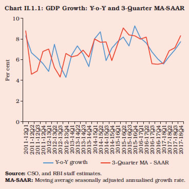

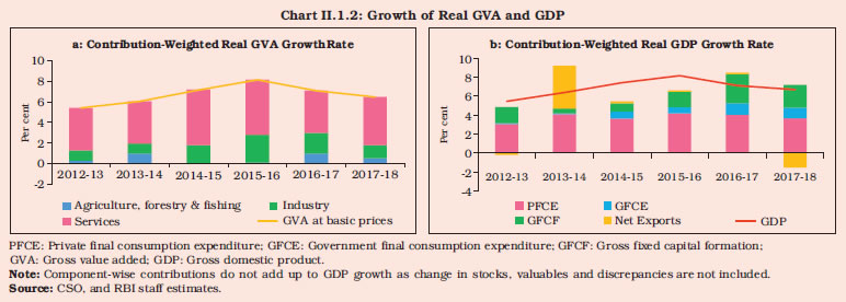II.1.6 Underlying the inflexion in aggregate demand conditions in 2017-18 were compositional shifts among constituents. Private final consumption expenditure (PFCE), which accounted for close to 57 per cent of real GDP growth in 2016-17, ceded share and its weighted contribution fell to around 55 per cent in 2017-18 (Chart II.1.2). While support from government final consumption was maintained at the preceding year’s level, net exports depleted domestic demand after remaining in broad balance a year ago. Gross fixed capital formation (GFCF) shed 7.6 percentage points in 2017-18 from its weighted contribution of 43.2 per cent to GDP growth in 2016-17. Nonetheless, the steady increase in its share in GDP growth from the low of 8.4 per cent in 2013-14 is noteworthy in view of its historical catalysing role in stepping up the pace of growth and its longer-lasting multiplier effects relative to other constituents, on the overall activity in the economy, employment and welfare.

Investment and Saving

II.1.7 This firming up of GFCF during 2017-18 acquires significance in the context of the recent experience which saw the rate of fixed investment, measured by the GFCF/GDP ratio, worsening steadily from 34.3 per cent in 2011-12 to 30.3 per cent in 2015-16. In 2016-17, however, GFCF shrugged off its secular decline and green shoots of revival became visible, led by private non-financial corporations and general government. Fixed investment of the private non-financial sector increased primarily in the form of machinery and equipment closely followed by intellectual property products. After a transient slowdown in Q1:2017-18 due to the lingering impact of demonetisation and uncertainties ahead of the implementation of the goods and services tax (GST), fixed investment rebounded in Q2 and sustained momentum over the rest of the year. The coincident turnaround in the growth of GDP and GFCF bears out the empirically validated switching role of the latter in turning points in the path of the Indian economy (Box II.1.1).

II.1.8 In terms of its determinants as employed by CSO, movements in GFCF appear to have been underpinned by the behaviour of domestic production of capital goods during the phase of a slowdown as well as the recent upturn from Q2:2017-18. As regards other drivers, viz., value added in construction turned up in the preceding quarter, but imports of capital goods lost strength from Q3 after a surge that started a year ago (Chart II.1.3).

Box II.1.1 Investment Climate for Growth: What are the Key Enabling Factors? The revival in gross fixed capital formation (GFCF) in the second half of 2017-18, has aroused considerable interest, with questions around its turning points and durability given that several lead/coincident indicators – sales growth, capacity utilisation, inventory drawdown, pricing power are also pointing to a much awaited upturn in the investment cycle. Growth in GFCF scaled a peak of 23.8 per cent in Q4:2009-10 before slackening significantly over a prolonged period thereafter (Chart 1) from an average rate of 11.7 per cent during 2005-06 to 2009-10 to 7.0 per cent during 2010-11 to 2017-18, with some intervening quarters registering contraction. Since Q2:2017-18, however, the growth of GFCF has picked up and sustained in Q3 and Q4 averaging 11.7 per cent. This development warrants an empirical assessment of the factors influencing the investment climate. The investment climate represents a combination of factors that includes macroeconomic and political stability, physical infrastructure, availability of financial capital and human resources, and the institutional, policy, and regulatory architecture. A transparent, stable and predictable investment climate is essential for growth and requires “…proper contract enforcement and respect for property rights, embedded in sound macroeconomic policies and institutions, transparent and stable rules, and free and fair competition” (IFC, 2016). Consequently, the business regulatory environment, taxation laws, and governance/institutional capacity often influence the ease and cost of starting a business as well as normal day-to-day operations. Quantitative and qualitative determinants of the investment climate have been captured in the form of a single index that helps identify the relative rank of a country, such as the ease of doing business index of the World Bank, competitiveness index (WEF, 2017), policy uncertainty index (Baker, et al., 2016), corruption index (Transparency International, 2018) and the like. 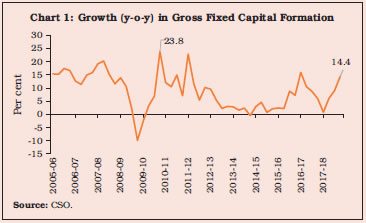For the empirical assessment, year-on-year (y-o-y) growth in real GFCF and the GFCF to GDP ratio were taken as dependent variables representing the realised investment climate, while y-o-y changes in the economic policy uncertainty index, the business expectations index in the RBI’s Industrial Outlook Survey and quarterly changes in the number of stalled projects are used as the measurable high frequency indicators of the investment climate. Drawing from the empirical literature, other determinants of the investment climate considered are the real interest rate representing the cost of finance, the real effective exchange rate as a proxy for competitiveness, and the profitability of current business indicating the return on investment (Table 1). The empirical estimation is based on the ordinary least square method, for the period 2001-02:Q1 to 2017-18:Q4 with heteroskedasticity and autocorrelation consistent (HAC) adjusted standard errors. A priori, it is posited that (a) greater the business optimism and lower the level of policy uncertainty, higher could be the appetite for new investment; (b) higher real interest rates and appreciation of the real effective exchange rate may dampen investment, unless the expected return on investment is high enough to improve the earnings outlook; (c) higher corporate profitability can drive higher investment; and (d) increase in the incidence of stalled projects can depress new investment activity. The empirical results point to persistence and gestation in the evolution of investment activity as evident in the statistically significant lagged dependent variable. This suggests that the investment climate is slow-moving and wields an influence on investment decisions. Consistent with expectations, policy uncertainties and bottlenecks (represented by stalled projects) have contributed to dampening of the investment climate. Corporate profitability, which is largely influenced by input costs and demand conditions that determine pricing power, emerges as a forward-looking driver of new investment. As current profits are expected to alter the earnings outlook or the expected return on new investment, higher profitability resulting from lower input costs, higher output prices or improved productivity could brighten the investment climate. Headwinds from factors like slow growth in demand represented by non-agricultural income, subdued business confidence, and higher real interest rates (i.e., the policy rate as well as the real weighted average lending rate) are seen to retard investment. An appreciation of the real exchange rate, which is an indicator of possible loss of external competitiveness, unless offset by higher productivity is found to adversely impact future investment demand (Table 1). Table 1: Factors that Influence the Investment Climate   Investment (INV) Growth in Real GFCF (y-o-y) GFCF to GDP Ratio 1 2 3 4 Constant -3.70 (-1.72)* 0.47 (0.22) 5.07 (4.66)*** INVt-1 0.51 (4.80)*** 0.39 (6.71)*** 0.77 (18.59)*** NAG_Gr t-1 0.98 (3.06)***     NAG_Gr t   0.50 (1.82)*   Real_int t-2 -1.55 (-3.03) ***     Real_int t-4   -0.65 (-1.99)**   Real_walr t-2     -0.09 (-2.81)*** DREER t-4 -0.23 (-2.04)**     DBEI t-1 0.44 (6.30)*** 0.33 (8.37)***   QBEI t-1     0.07 (5.14)*** DUNCRT t-4 -0.02 (-1.92)**     EBITDA t-1   0.14 (3.88)***   PROFIT t-1     0.18 (3.44)*** DSTALLED t-5     -0.01 (-2.24)** R2 0.67 0.76 0.94 LB-Q (P-value) 0.10 0.33 0.27 Notes: 1. ***; **; *: indicate the statistical significance at 1 per cent, 5 per cent and 10 per cent, respectively. 2. Figures in parentheses are t-statistics. 3. LB-Q is Ljung-Box Q statistics for the test of null hypothesis of no serial correlation (up to 5 lags). 4. Dependent variable in Col. (2) and (3) is year-on-year growth in real GFCF while that in Col. (4) is GFCF to GDP ratio. NAG_Gr : Non-agricultural real GDP growth (y-o-y) Real_int : Change in real policy rate Real_walr : Real weighted average lending rate DREER : Change (y-o-y) in Real Effective Exchange rate DBEI : Change (y-o-y) in Business Expectations Index (From RBI’s Industrial Outlook Survey) QBEI : Deviation of Business Expectations Index from 100 level (From RBI’s Industrial Outlook Survey) DUNCRT : Change (y-o-y) in economic policy uncertainty index (Source: www.PolicyUncertainty.com). EBITDA : Change (y-o-y) in earnings before interest, taxes, depreciation and amortisation adjusted for inflation. PROFIT : Net profits (profits after tax) to sales ratio. DSTALLED : Quarterly change in stalled projects (numbers). Source: RBI staff estimates. These empirical findings indicate that a combination of factors work to ensure a durable improvement in the investment climate, and, in turn, the rate of investment in the economy. References: 1. Baker, S. R., N. Bloom and S. J. Davis (2016), “Measuring Economic Policy Uncertainty”, The Quarterly Journal of Economics, Vol. 131, No. 4, pp. 1593–1636. 2. International Finance Corporation (IFC) (2016), “The Investment Climate”, Issue Brief Series, July, IFC. 3. Transparency International (2018), “Corruption Perceptions Index 2017”, Available at: https://www.transparency.org/news/feature/corruption_perceptions_index_2017. 4. World Economic Forum (2017), “The Global Competitiveness Report 2017–2018”, September, Geneva.

II.1.9 Construction activity remained subdued in 2016-17 with Q4:2016-17 recording a contraction. Recent structural reforms in the sector such as Real Estate (Regulation and Development) Act, 2016, might have produced some initial retardation before beneficial effects set in. However, this sector accelerated in Q3:2017-18 and grew by 11.5 per cent in Q4:2017-18, the highest in the 2011-12 base year series. This was also mirrored in proximate coincident indicators – steel consumption and cement production. Cement production, which contracted in seven successive months starting in December 2016, has started showing double digit growth since November 2017. Around two-thirds of cement demand emanate from the housing and real estate sector.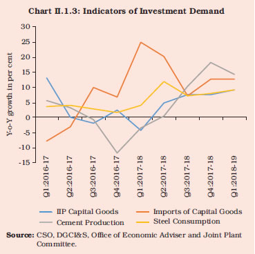

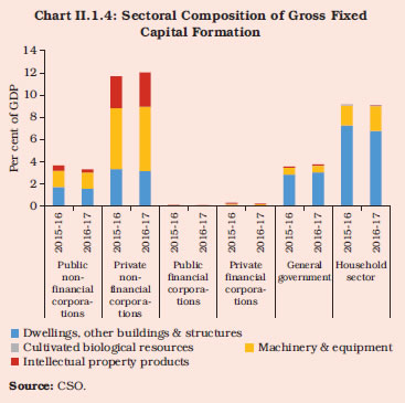II.1.10 The share of fixed investment in dwellings, buildings and other structures dropped from 16.3 per cent of GDP in 2015-16 to 15.7 per cent in 2016-17, primarily in the household sector, followed by public non-financial corporations (Chart II.1.4). This was, however, compensated by fixed investment in machinery and equipment whose share rose from 10.6 per cent of GDP in 2015-16 to 11.9 per cent in 2016-17. Constrained by the rigidities confronting the domestic supply of capital goods cited above, domestic demand has increasingly spilled over into imports, resulting in the phenomenon of reverse substitution of domestic production by imports.

II.1.11 The Reserve Bank’s Order Books, Inventories and Capacity Utilisation Survey (OBICUS) points to a pick-up in capacity utilisation in manufacturing alongside a drawdown in finished goods inventories from Q2:2017-18. The Industrial Outlook Survey (IOS) indicates that business optimism picked up relative to preceding quarters, mainly contributed by positive assessments on production, order books, capacity utilisation, employment, imports and exports. There has also been a gradual return of pricing power of manufacturing enterprises since Q3:2017-18. Stalled projects, both in numbers and value, declined in Q1:2018-19; however, new investments remained lukewarm uniformly across the government and the private sectors (Chart II.1.5). The plant load factor (PLF) in thermal power plants remained at the same level as in the previous year at about 60 per cent. Greater competition from renewable energy sources is increasingly evident.

II.1.12 The infrastructure sector, which is a key barometer of the investment climate, reflects the green shoots of strengthening capital formation in the economy after a hiatus. First, the length of highway projects constructed during 2017-18 maintained its growth momentum by increasing to 9,829 km from 8,232 km in the previous year. The length of highway projects awarded during 2017-18 increased to 17,055 km from 15,949 km in the preceding year. Second, a large part of the railway capex in 2017-18 was devoted to doubling or trebling of lines, gauge conversion and electrification. A key development was the laying down of the foundation for the Mumbai-Ahmedabad bullet train project. Third, in order to cater to surging domestic air traffic, the government has awarded flight routes to various underserved and unserved airports along with viability gap funding. Fourth, re-rating of the capacities of major ports in India showed an increase in rated capacity from 1,066 to 1,359 million tonnes per annum. Fifth, the government has launched the Pradhan Mantri Sahaj Bijli Har Ghar Yojana (SAUBHAGYA) with the target of universal household electrification by March 2019.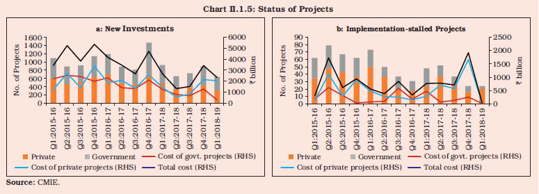

Consumption

II.1.13 As in the past, consumption remained the dominant component of aggregate demand in 2017-18, accounting for 66.6 per cent of GDP. Consumption expenditure has provided valuable support to aggregate demand through the recent slowdown, including by cushioning the shocks imparted by demonetisation and the implementation of GST. In fact, the period 2013-17 is characterised as one of consumption-led growth (RBI Annual Report, 2016-17) as it contributed 64.4 per cent of the change in GDP during these years. In particular, GFCE, buoyed by enhanced salaries, pensions and allowances under the 7th central pay commission’s award for central government employees and the one rank one pension award for defence personnel, has operated like a fiscal stimulus in a period of sluggish demand in the economy. If GFCE is excluded, the average growth of GDP of 6.9 per cent during 2016-18 would slump to 6.4 per cent. The evolution of GFCE is sketched out within a fuller analysis of public finances in section II.5.

II.1.14 PFCE, the mainstay of aggregate demand in India, slowed down in 2017-18, with the deceleration more pronounced in the first half of the year. The loss of speed in PFCE reflected a combination of factors – the overhang of demonetisation, especially in respect of the unorganised sector; the initial disruptions associated with the implementation of GST; and some deceleration in rural wage growth.

II.1.15 Domestic saving declined to 29.6 per cent of gross national disposable income (GNDI) in 2016-17 from 30.7 per cent in 2015-16 (Appendix Table 3). Household financial saving – the most important source of funds for investment in the economy declined to 6.7 per cent of GNDI in 2016-17, down from 8.1 per cent in 2015-16 (Table II.1.1). Saving of private non-financial corporations dropped marginally to 11.1 per cent of GNDI in 2016-17. At the same time, general government’s dissaving declined to 0.7 per cent in 2016-17 indicating sustained efforts to bring fiscal consolidation. As per the Bank’s preliminary estimates, net financial assets of the household sector increased to 7.1 per cent of GNDI in 2017-18 on account of an increase in households’ assets in the form of currency, despite an increase in households’ liabilities.

Aggregate Supply

II.1.16 Aggregate supply, measured by gross value added (GVA) at basic prices expanded at a slower y-o-y pace in 2017-18, 0.6 percentage points down from 7.1 per cent in the preceding year and 0.9 percentage points below the decennial trend rate of 7.4 per cent (Appendix Table 2). Disentangling momentum from base effects, it is interesting to observe that while momentum registered an uptick in Q2, providing a much needed thrust to growth, base effects also came into play in H2. For the year 2017-18 though, annual growth rates obscure an important turning point that is picked up in quarterly changes. In terms of y-o-y quarterly growth rates, a loss of speed is discernible from Q1:2016-17 which persisted right up to a thirteen-quarter low in Q1:2017-18. In Q2, however, a turnaround – essentially powered by a surge in industrial activity – took hold, and as the agriculture and services sector joined in, GVA growth continued to accelerate in Q3 and Q4. GVA momentum, measured in terms of q-o-q seasonally adjusted annualised growth rate (SAAR), showed a marked improvement from Q2:2017-18. Services, which comprise over three-fifths of GVA rebounded in 2017-18 with a broad-based growth across sub-sectors (Table II.1.2).

II.1.17 The disconnect between annual and quarterly growth rates in capturing the shifts in GVA in 2017-18 is evident in each constituent. In respect of agriculture and allied activities, GVA grew by 3.4 per cent in 2017-18 on top of record levels of foodgrains and horticulture output that fuelled a growth of 6.3 per cent a year ago. In terms of quarterly growth rates, however, a pick-up is evident in H2:2017-18. The reasonably satisfactory rabi harvest is reflected in the growth of agriculture GVA at 4.5 per cent in Q4:2017-18. Nonetheless, the contribution of agriculture and allied activities to real GVA growth declined to 7.9 per cent from 13.6 per cent in 2016-17.

II.1.18 To situate this assessment in some perspective, the southwest monsoon arrived two days ahead of schedule in 2017 and ten days earlier than last year, but it lost momentum during mid-July and August and this took a toll on sowing acreage in the season as a whole. Eventually, precipitation for the season as a whole was only 5 per cent below the long period average (LPA), but knock-on effects of the mid-season dry spell led to merely 0.3 per cent growth over the last year in kharif foodgrain production. Yet, it is important to note that the output level achieved in 2016-17 was an all-time record. If the 2017-18 kharif performance is evaluated against that backdrop, all crops grew by more than 10 percentage points over the average of the last 10 year production. Among cash crops, sugarcane and cotton production exceeded the preceding year’s level but jute and mesta output dropped marginally.

II.1.19 Turning to the rabi season, the delayed retreat of the southwest monsoon led to late sowing. Moreover, the progress of rabi sowing was hindered by the uncertainty surrounding stubble burning and the sudden onset of cold conditions during January 2018. The deep deflation in the prices of pulses, oilseeds and several perishables also dis-incentivised acreage expansion in these crops. Ultimately, the northeast monsoon season ended with a rainfall deficiency of 11 per cent below the LPA, but supported by comfortable levels of water in major reservoirs, sowing managed to survive the vicissitudes of weather and was just 0.8 percentage points lower than last year’s level.

II.1.20 Overall, India is set for a record foodgrain output in the crop year ending June 2018 increasing by 1.6 per cent y-o-y to a level of 279.5 million tonnes (Table II.1.3). The output of rice, wheat, pulses and coarse cereals is expected to have achieved record levels in 2017-18, while oilseeds production declined on account of lower production of soyabean.

II.1.21 In the current southwest monsoon season so far (upto August 17, 2018), rainfall was 8 per cent below the LPA and 26 subdivisions covering 78 per cent of the area received excess/ normal rainfall. As a result, water level in 91 major reservoirs in the country replenished and turned out higher than the previous year’s level. However, the kharif sowing so far is lower by 1.5 per cent compared to the last year’s acreage.

Horticulture

II.1.22 Horticulture output has expanded significantly over the last few years. Accounting for 34 per cent of the value of output from crops (average over 2011-16), horticulture has imparted stability to agricultural output. In 2017-18, horticulture production touched a record level of 307.2 million tonnes, up by 2.2 per cent over the level in 2016-17. The production of fruits and vegetables increased y-o-y by 1.6 per cent and 2.2 per cent, respectively. Among the three key vegetables, the production of potato and tomato increased, while the production of onion declined during the year, mainly on account of lower acreage. The rise in horticulture productivity was not sustained in 2017-18, with the per acre production decreasing marginally by 0.06 per cent.

Allied Activities

II.1.23 Allied activities, which include forestry, fishing and livestock contribute around 39 per cent of the gross output in agriculture and allied activities. In order to promote allied activities, the government has set up an Animal Husbandry and Infrastructure Development Fund (AHIDF) for financing infrastructure requirements of the animal husbandry sector. The facility of Kisan Credit Card has been extended to the fisheries and livestock farmers. A National Mission on Bovine Productivity helps to reach the benefits of animal husbandry to farmers directly. The five year average growth (2012-13 till 2016-17) of allied activities has stepped up to 5.6 per cent, well above the quinquennial average growth of 2.7 per cent for the sector of agriculture and allied activities as a whole.

e-NAM

II.1.24 In order to create a unified national market for agricultural commodities, e-NAM, the e-trading platform for the National Agriculture Market was launched in April 2016 and its reach has been expanded considerably over the last two years. The platform now covers 585 markets across 16 states and two Union Territories (UTs) as on June 30, 2018 (Chart II.1.6). The total cumulative value of trade under e-NAM since the time of its launch has reached ₹482.15 billion, and 10.7 million farmers, 63,059 commission agents and over 0.1 million traders have registered on the e-NAM platform so far.

II.1.25 The scheme has immense potential to transform the agricultural marketing structure through smoother inter-state movements, more efficient price discovery and removal of intermediaries. The adoption process, however, has been slow and gradual with a majority of traders/farmers still continuing with the manual auction method for selling their products. Recent initiatives to boost e-NAM include: (a) simplifying registration of farmers on the portal, (b) expanding payment options (addition of Unified Payment Interface) and (c) extending e-NAM trading in six languages. Measures such as third-party assaying, quality certification mechanisms, dispute settlement mechanisms and digital infrastructure will improve the adoption of e-NAM considerably.

Union Budget 2018-19 Proposals

II.1.26 The Union Budget 2018-19 has proposed a number of measures to enhance rural income and promote agriculture, viz., (i) setting the minimum support prices (MSPs) for crops at 1.5 times the cost of production; (ii) setting up an Agri-Market Infrastructure Fund with a corpus of ₹20 billion for developing and upgrading agricultural marketing infrastructure in the 22,000 Grameen Agricultural Markets (GrAMs) and 585 Agricultural Produce Market Committees (APMCs); (iii) creation of a Fisheries and Aquaculture Infrastructure Development Fund (FAIDF) and the AHIDF; (iv) launching a re-structured National Bamboo Mission with an outlay of ₹12.9 billion to promote the bamboo sector in a holistic manner; (v) launching an ‘‘Operation Greens’’ along the lines of ‘‘Operation Flood’’ to promote Farmer Producers Organisations (FPOs), agri-logistics, processing facilities and professional management; (vi) further expansion of the ground water irrigation scheme under the Pradhan Mantri Krishi Sinchayee Yojana - Har Khet ko Pani; and (vii) providing health protection cover of ₹0.5 million each for 100 million poor and vulnerable families.

II.1.27 Currently MSPs for 23 agricultural commodities of kharif and rabi seasons are announced by the government, based on recommendations of the Commission for Agricultural Costs and Prices (CACP). Procurement at MSP is, however, largely restricted to rice (kharif season) and wheat (rabi season). As a result, the weighted average mandi prices trade below the MSP for many of the crops, e.g., urad, tur, chana, lentil, maize, groundnut, soyabean, bajra, rapeseed and mustard, causing loss to farmers. In line with the announcement in the Union Budget, the Government has recently fixed MSP for several kharif crops for the sowing season of 2018-19 which ensures a return of at least 50 per cent over the cost of production (as measured by A2 plus FL¹). A few state governments have also launched their own price support schemes/financial assistance for farmers.

Farm Loan Waivers

II.1.28 In order to address growing farmers’ distress, several state governments, viz., Uttar Pradesh, Punjab, Maharashtra, Rajasthan and Karnataka have announced farm loan waivers.

While waivers may cleanse banks’ balance sheets in the short-term, they may dis-incentivise banks from lending to agriculture in the long-term (EPW Research Foundation 2008; Rath 2008)².

Industrial Sector

II.1.29 GVA growth in industry decelerated on a y-o-y basis to 5.5 per cent in 2017-18 in a sequence that commenced a year ago when it came off a recent peak of 12.1 per cent in 2015-16. Consequently, the weighted contribution of industry to overall GVA growth declined from 33.5 per cent in 2015-16 to 20.0 per cent in 2017-18. Also, the cyclical component of growth (estimated through a univariate approach using the Hodrick-Prescott filter) turned negative in 2017-18 and capacity utilisation in the manufacturing sub-sector remained below the 10-year average (Chart II.1.7 a and b).

II.1.30 On a seasonally adjusted three-quarter moving average annualised basis, industrial GVA growth recovered sharply in Q2 and maintained an upward trajectory thereafter. Similarly, seasonally adjusted industry GVA showed that the revival in industrial activity in 2017-18:Q2-Q4 was primarily driven by momentum.

II.1.31 As stated earlier, annual changes mask the inflexion points in the evolution of industrial output during the course of the year. Quarterly growth rates reflected a protracted slowdown that started during Q2:2016-17 and slid into a contraction in Q1:2017-18. In Q2, however, there was a rebound driven by manufacturing and electricity generation, which helped the overall value added to shrug off the drag from mining. Over H2:2017-18, the tempo of expansion in industrial GVA was sustained on the shoulders of an acceleration in manufacturing, despite the support from the electricity sub-sector moderating and a slump in mining output.

II.1.32 The deceleration in the growth of GVA in industry in 2017-18 in relation to the preceding year is also reflected in the index of industrial production (IIP), although intra-year movements in industrial output reflected an underlying improvement gathering (Table II.1.4). At a sectoral level, the recovery was witnessed in the manufacturing sector, while mining and electricity sectors decelerated. In 2018-19 so far (April-June), industrial activity improved on the back of manufacturing and mining even though electricity generation expanded at a subdued pace. In terms of use based activity, primary goods, capital goods, consumer durables and infrastructure/construction goods contributed to the acceleration in the IIP growth.

II.1.33 While mining and quarrying output has been considerably volatile in recent years on account of commodity-specific constraints, favourable base effects enabled a pick-up in Q2 from a flatter outcome in the preceding quarter. The upturn was short-lived, however, as coal and natural gas production fell off and crude oil output declined. Coal output decelerated for three successive years (2015-16 to 2017-18). Consequently, the reliance on imported coal for thermal power plants has reduced only marginally. The planned production ramp-up by Coal India Limited (CIL) has been hit by ageing mines, depleting resources and rising output costs with a progressively increasing strip ratio³. Recent initiatives to allocate additional coal mines and easing regulations for coal-bed methane extraction could boost CIL’s output. The output of fossil fuels, viz., crude oil and natural gas, has been constrained by the natural decline in extraction from ageing oil fields and factors like uncertain price policy, power shut downs, water cuts, and labour related frictions. Iron ore has been the clear bright spot in mining commodities in recent years, and its output growth in 2017-18 remained strong despite disruptions in the major mining states of Odisha and Goa. The growth in iron ore mining was helped by the underlying growth of steel demand, both domestic and global; favourable commodity prices and trade policy interventions.

II.1.34 The recovery in manufacturing was broad-based with production in 15 industry groups out of the total of 23 industry groups expanding during H2:2017-18 vis-à-vis only 10 industries during H1. By Q3, the combined contribution of items that registered expansion had decisively reversed the five preceding quarters of decline.

II.1.35 Among the major industry groups, coke and refined petroleum, chemical and chemical products, food products, machinery and equipment and other non-metallic mineral products together accounted for 33.8 per cent of the IIP, which witnessed a turnaround in performance. Pharmaceuticals registered the highest growth rates driven by digestive enzymes and antacids (DEAs). Electrical equipment has remained in contraction mode through Q1-Q4:2017-18.

II.1.36 Indicators of financial performance of listed manufacturing firms reveal that the deceleration in sales growth in Q1:2017-18 – possibly due to GST-induced de-stocking by downstream distribution channels – reversed thereafter and sales growth rebounded in Q2-Q4. Moreover, a slow return of pricing power is also taking root amidst rising input cost pressures; consequently, profit margins are improving (Chart II.1.8a). Indicators of operational performance from the RBI’s OBICUS survey point to a reduction in inventory levels for manufacturing firms in Q4:2017-18. Also, the capacity utilisation level improved in Q2-Q4:2017-18 after deteriorating marginally in Q1:2017-18 (Chart II.1.8b).

II.1.37 As regards expectations, manufacturing firms polled in the RBI Industrial Outlook Survey turned optimistic in Q3-Q4:2017-18, though the expectations for Q1-Q2:2018-19 dipped due to weaker prospects for production, order books, profit margins and overall financial situation.

II.1.38 Electricity generation began on a strong note with sequential acceleration in H1 of 2017-18 on the back of a revival in demand from Distribution Companies (DISCOMs). Demand accelerated in Q3 as a strong pick-up in manufacturing joined a situation in which supply was unable to keep pace, increasing the power deficit. In Q4 though, supply accelerated, reducing the power deficit (Chart II.1.9). Demand-supply dynamics were reflected in spot prices peaking in Q3:2017-18 on the Indian Energy Exchange, when the power deficit was the highest.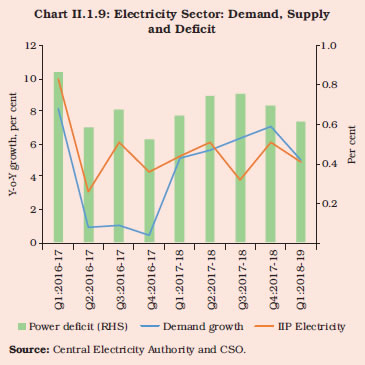

II.1.39 In terms of sources, thermal power, which has the highest share, was beset with challenges impacting both demand and supply. On the demand side, financial vulnerability of DISCOMs has constrained offtake and led to aversion to enter into new long-term power purchase agreements (PPAs). Some DISCOMs have defaulted on such existing agreements, substituting them with lower cost spot-market purchases. Ujwal DISCOM Assurance Yojana (UDAY) has yielded some results in bridging the gap between aggregate cost of supply and aggregate revenue realised through interventions in lowering finance costs, reducing aggregate technical and commercial losses, and increasing prices for the domestic segment. However, the progress has been uneven across states with spillover effects for power generation companies – particularly for thermal power plants with high-cost PPAs. Excess capacity continues to persist in the thermal power sector (especially in the private sector) with plants operating at sub-optimal plant load factor (PLF) that in turn could undermine their financial viability going forward.

II.1.40 Renewable energy has seen higher consistent growth during the year. Over the last 10 years, installed capacity increased almost 6 times – from 11.1 GW in 2007-08 to 65.5 GW in 2017-18 – and its share in power generation increased from 3.0 per cent in 2007-08 to 7.1 per cent in 2017-18. The composition of renewable energy itself is undergoing structural change, with the share of solar rising sharply to around 24 per cent in 2017-18 from a negligible level in 2007-08. The higher growth in renewables is in part driven by emissions targets committed under the Paris Climate Accord. Photo-Voltaic (PV) cell costs have declined sharply with increasing technology maturity and scale of production. The renewable energy target set by the government (175 GW installed capacity by 2022) gives the highest priority to solar energy (100 GW installed capacity). India has taken the lead in international co-operation for solar energy development, by taking a leadership role in establishing the International Solar Alliance (ISA), a platform for sharing affordable technology and mobilising low-cost finance among member nations. The ISA has set a target of 1 Terawatt (TW) of solar energy by 2030. As the host and secretariat to ISA, India will provide 500 training slots for ISA member countries and start a solar tech mission to lead research and development (R&D).

II.1.41 On a use-based classification, IIP growth in H1:2017-18 was primarily attributable to primary goods and consumer non-durables. By contrast, the acceleration in H2 was driven by capital goods, infrastructure/construction goods and intermediate goods.

II.1.42 Capital goods output – considered an indicator of capital formation/investment – recovered from contraction mode since September 2016 (barring expansion in November 2016 and March 2017) and expanded for seven successive months since August 2017. Transportation and manufacturing sector related investment goods like commercial vehicles and vehicle parts, tyres, ship building, separators and sugar machinery were the drivers. Infrastructure/construction goods expanded in H1, with strong growth in iron and steel related products outweighing the contraction in cement production. The segment regained strength and posted acceleration in H2 due to a sharp pick-up in cement production and continued strong growth in iron and steel on progress in government driven infrastructure projects, including affordable housing.

II.1.43 Consumer non-durables, the strongest driver from the use-based side was heavily influenced by pharmaceuticals, in particular, DEAs. Excluding DEAs, this category would have contracted in H1, although components within the food and beverages industry group like sugar, milk, poultry meat and shrimps revived activity in the category in H2. Consumer durables output resumed growth from November 2017 onwards after contraction in 9 out of previous 11 months. In the case of intermediate goods, output growth closely followed that of manufacturing.

Services Sector

II.1.44 In contrast to the industrial sector, the services sector growth accelerated on a y-o-y basis to 7.6 per cent in 2017-18 breaking the sequence of two years of deceleration. Also, excluding the government driven PADO component, service sector growth rate accelerated from 5.7 per cent in 2016-17 to 7.0 per cent in 2017-18. Nevertheless these growth rates remain significantly lower than the recent high of 9.3 per cent (2014-16).

II.1.45 On a seasonally adjusted three-quarter moving average annualised basis, services GVA growth (excluding PADO) recovered sharply in Q1, influenced by the acceleration in trade and real estate segments due to the push to clear inventories before the GST launch. Seasonally adjusted and decomposed into momentum (q-o-q changes) and base effects, the momentum achieved in Q1 weakened in the subsequent quarters.

II.1.46 The recovery in services GVA was fairly broad-based across constituent sub-sectors (Chart II.1.10a). In terms of weighted contribution to growth, that of PADO declined marginally in 2017-18, while all other sub-sectors witnessed improvement (Chart II.1.10b).

II.1.47 The CSO’s initial GVA estimates of the services sector are based on the benchmark-indicator method. Construction GVA accelerated in 2017-18 with steel consumption growing at a sustained pace throughout and cement production accelerating in Q3-Q4. The key drivers were government infrastructure projects.

II.1.48 Trade, hotels, transport, communication and services related to broadcasting posted robust growth which was sustained through the year, visible also in the performance of coincident indicators⁴. Trade and transport are the biggest components, accounting for 59 per cent and 26 per cent, respectively, of this sub-sector. In the transport segment, railways, road and services incidental to transport are the biggest sub-components with shares of 15 per cent, 66 per cent and 16 per cent, respectively. Under rail transport, net tonne kilometres (70 per cent weight) registered significant acceleration in H2 while passenger traffic (30 per cent weight) growth remained subdued throughout the year. In the road transport segment, the stock of commercial vehicles on road accelerated from Q2:2017-18 onwards, with sales of new commercial vehicles showing robust growth. The acceleration observed in transport sector indicators during 2017-18 continued in Q1:2018-19, reflected in both rail freight traffic and commercial vehicle sales.

II.1.49 The major components of financial, real estate and professional services sub-sector are ownership of dwellings (29 per cent), financial services (28 per cent share) and IT services (21 per cent). Under financial services, bank credit accelerated significantly in H2 after a subdued performance in the preceding half. Aggregate deposits, in contrast, decelerated sharply in H2 after registering strong growth in H1:2017-18. In the case of IT services, the resilient EBITDA posted a growth of 5.7 per cent while the growth in staff costs was broadly positive in 2017-18. Exports of software services showed improvement though they faced uncertainties from visa policies in the United States and Australia. PADO continued to provide an upward thrust to the sector.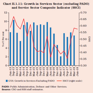

II.1.50 The Reserve Bank’s service sector composite index (SSCI), which extracts and combines information collated from high frequency indicators and statistically leads GVA growth in the services sector turned up in Q3:2017-18 (Chart II.1.11). A downward tendency in SSCI for Q1:2018-19, may be indicative of subdued services sector activity.

Employment

II.1.51 Formal sector employment, compiled from payroll data (Employees’ Provident Fund Organisation, Employees’ State Insurance Corporation and National Pension System) points towards an improvement in jobs created in 2017-18 vis-à-vis 2016-17. Total new subscribers (combined for the aforementioned three schemes) added per month improved from 1.6 million in 2016-17 to 1.8 million in 2017-18. Further, the Labour Bureau Quarterly Employment Survey, which measures addition to employment in the organised sector across eight sectors, indicates an incremental employment of 0.2 million in 2017-18 (up to September) which was higher than Q1-Q2:2016-17 by 0.9 lakhs.

II.1.52 The Union Budget 2017-18 had emphasised on energising of the youth through education, skills and jobs. The Skill India Mission launched in July 2015 to maximise the benefits of a huge demographic advantage was intensified by the Skill Acquisition and Knowledge Awareness for Livelihood Promotion Programme (SANKALP) launched at a cost of ₹40 billion in 2017-18. It is expected to provide market relevant trainings to around 35 million youth. Further, the next phase of Skill Strengthening for Industrial Value Enhancement (STRIVE), launched at a cost of ₹22 billion in 2017-18 with a focus on improving the quality and market relevance of vocational trainings provided in it, would strengthen the apprenticeship programmes through an industry cluster approach. A special scheme for creating employment in the textile sector has already been launched, and a similar scheme was to be implemented for leather and footwear industries in 2017-18.

II.1.53 Going forward, the focus of Union Budget 2018-19 on certain sectors such as agriculture, infrastructure, small and medium enterprises (SMEs) and also rural areas in general may provide a further fillip to consumption demand. The expected normal southwest monsoon in 2018 may also facilitate in keeping rural demand at an elevated level.

II.1.54 To sum up, economic activity in the Indian economy exhibited resilience in the face of several shocks during the year – demonetisation’s after effects; GST implementation; spillovers from global sell-offs in bonds and equities; bouts of capital outflows; frauds in domestic banking system amidst mounting loan delinquencies and capital constraints; and the ongoing terms of trade erosion. In this setting, loss of speed in GDP growth of 0.4 percentage points in relation to the preceding year notwithstanding, India’s real GDP growth at 6.7 per cent was still among the highest for major continental-sized economies in the world. In the second half of the year, the impact of these drag factors started gradually dissipating and average real GDP growth accelerated to 7.4 per cent, exceeding the annual pace of growth in 2016-17. Importantly from a forward looking perspective, several turning points were passed in various quarters during the year – notably, gross fixed investment on the demand side, and on the supply side, manufacturing in industrial activity and construction in services. If these inflexions take firmer hold, they should support an enduring acceleration of momentum in the economy and spur an expansion into employment and incomes all around.

II.1.55 Agriculture and allied activities have provided a solid foundation to the Indian economy, especially in a year marked by several shocks (as alluded to earlier). A second successive year of bumper production of foodgrains and horticulture on the back of reasonably good monsoons has not, however, translated adequately into a boost to farm and rural incomes. Adverse and worsening terms of trade and high variability in the access to international markets has sapped away the large gains in production.

II.2 PRICE SITUATION

II.2.1 A distinctive feature of the evolution of headline inflation⁵ during 2017-18 has been its high variability, notwithstanding lower average inflation relative to its history through the new series (Table II.2.1). Against this backdrop, sub-section 1 discusses the movements in headline inflation through three phases during the year, with food inflation playing an important role in both disinflationary and reflationary periods. Sub-section 2 assesses global inflation developments, which is followed by a detailed analysis of the major constituents of inflation in sub-section 3, with an emphasis on the drivers of food, fuel, and excluding food and fuel inflation. Sub-section 4 discusses other indicators of inflation such as sectoral consumer price index (CPI), wholesale price index (WPI), and GDP deflators as well as movements in wages – both rural wages and corporate staff costs. Sub-section 5 provides some concluding observations.

1. Headline CPI Inflation

II.2.2 In a surprise relative to expectations and consensus forecasts, inflation fell off the precipice in Q1 under the weight of overhang of the supply glut in inflation-sensitive food items, notably pulses and oilseeds, as well as higher mandi arrivals of some vegetables such as potatoes and onions. In the event, instead of the usual pre-monsoon upturn, food prices sank into deflation, taking headline inflation down into a temporary breach of the tolerance floor of the inflation target band. At 1.5 per cent in June 2017, it was the lowest reading in the new CPI series. Moreover, continuing deflation in the prices of pulses and spices (during June-March, 2017-18), along with moderation in prices of overall food and miscellaneous components imparted a negative skew to headline inflation, as against a positive skew during 2016-17.

II.2.3 From July, a confluence of domestic and global developments propelled headline inflation up by 375 basis points (bps) to 5.2 per cent in December 2017, a 17-month high (Chart II.2.1). Just as in the disinflation phase, the reflation was led by prices of vegetables, particularly of tomatoes and onions. The disbursement of house rent allowance (HRA) for central government employees under the 7th Central Pay Commission’s award added momentum. In particular, the prices of vegetables surged in an unseasonal spike during October-November due to the late withdrawal of southwest monsoon leading to the damage of some crops. The usual seasonal softening in food prices with the arrival of the winter harvest finally occurred with a delay in December which, together with pro-active supply management measures adopted by the government – import of onions and imposition of a minimum export price (MEP) – helped contain price pressures and headline inflation ebbed to 4.3 per cent in March 2018. Excluding the effect of the HRA, it was even lower at 3.9 per cent. Strikingly, the weighted contribution of inflation excluding food and fuel to headline inflation jumped up in Q3:2017-18 and persisted at elevated levels through March 2018 with signs of a closing output gap and rising capacity utilisation.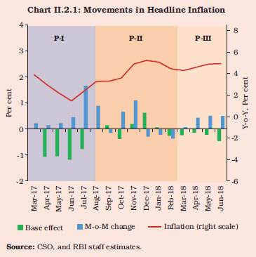

II.2.4 For the year as a whole, inflation came down on an annual average basis to 3.6 per cent in 2017-18, around 90 bps lower than a year ago. Excluding the impact of HRA, annual average inflation during 2017-18 stood at 3.4 per cent (Table II.2.1). The decline was not broad-based though, with housing and fuel inflation increasing in 2017-18 (Appendix Table 4). On several occasions during the year, households looked through transient falls in their inflation expectations formation, suggesting that adaptivity is slowly giving way to forward-looking behaviour, in line with the broad consensus in the literature⁶.

II.2.5 According to the March 2018 round of the Reserve Bank’s survey, inflation expectations remained elevated for both three months ahead and a year ahead horizons. This is also corroborated by more forward-looking professional forecasters in the Reserve Bank’s March 2018 round of the survey of professional forecasters.

II.2.6 Beginning 2018-19, headline inflation picked up during Q1:2018-19 largely led by increase in prices within food, fuel and miscellaneous sub-groups. While price pressures were broad-based in case of miscellaneous component, within food group upside pressures primarily emanated from vegetables and select protein-rich items like meat and fish.

2. Global Inflation Developments

II.2.7 Domestic inflation developments acquire contextual relevance when they are situated in a global perspective. Globally, prices of agricultural commodities, especially of food items such as cereals, sugar and edible oils like soyabean remained broadly soft during the year, reflecting abundant supply. In the non-food category, metal prices hardened due to strong demand from China, which accounts for more than half of global consumption. Global crude oil prices were supported by the decision of the Organisation of the Petroleum Exporting Countries (OPEC) and non-OPEC producers – led by Russia – in November 2017 to extend the cut in oil production by 1.8 million barrels per day till the end of 2018. The price of the Indian basket of crude oil moved in tandem and rose to US$ 64 per barrel in March 2018 from US$ 51 per barrel in March 2017.

II.2.8 Against this backdrop, an interesting development has been that even as inflation has picked up with economic recovery in advanced economies during 2017, it has eased in emerging and developing Asia despite stable economic growth and rising global commodity prices, suggesting an important role for inflation targeting (IT) as a monetary policy framework and its gradual refinements over the years in a number of Asian economies (Box II.2.1).

3. Constituents of CPI Inflation in India

II.2.9 Circling back to the domestic price front, intra-year movements in headline inflation were underpinned by significant shifts at the sub-group level (Chart II.2.2). Subsequent paragraphs will profile the key drivers of the collapse of food inflation in the first half of the year and its surge in the second half, the sustained increase in fuel inflation from Q2 albeit with some moderation in Q4, and the upturn in inflation in ‘excluding food and fuel category’ during the second half of the year causing it to exceed 5 per cent from December 2017 and to rule above headline all through March 2018.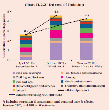

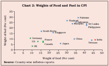
Box II.2.1 Inflation in Asia after the Global Financial Crisis - How is it Different from the Rest of the World? While the advanced economies have witnessed a pick-up in inflation along with economic recovery, after a prolonged period of deflationary risks, emerging market and developing economies (EMDEs) as a group, and emerging and developing Asia7 in particular, have continued to record moderation in inflation (Charts 1.a & 1.b). A cross-country comparison of weights of fuel and food in the CPI shows that the weights are generally higher in select Asian economies than in advanced economies (Chart 2). Therefore, the impact of rising global fuel and food prices since 2015 should have resulted in rising inflation (instead of moderation) in Asia. 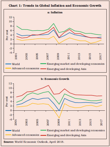Against this backdrop, the underlying drivers of inflation in Asia were examined in a panel framework. The data set included eleven Asian economies of which six are inflation targeters8 and five advanced economies among which Canada, UK, Germany and France (as part of the euro area) are inflation targeters. Drawing from the literature (Fraga et al, 2003; Mishkin and Hebbel, 2001), a dynamic panel data model in equation (1) with the Arellano-Bover/Blundell-Bond system generalised method of moments (GMM) estimation was carried out on a panel comprising annual data for the 16 economies for the period 1990 to 20179. The base model (1) aims at analysing the impact of the adoption of inflation targeting (IT) (modelled as a dummy variable taking the value 1 from the adoption year of IT and value 0 in the pre-IT years) on inflation for the entire set of countries while controlling for factors like the output gap and its lag, the fiscal deficit, the exchange rate (expressed in local currency unit per US$), global energy prices and import share in GDP. While the IT dummy, import share and global energy price inflation were considered to be exogenous variables in the model, the output gap, the fiscal deficit and the exchange rate were treated as endogenous10: 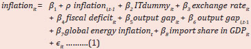Table 1: Results of the Dynamic Panel Data Models11 Explanatory Variables 16 Countries: 1990-2017 Dependent Variable: Inflation 11 Asian Countries: 2001-2017 Dependent Variable: Inflation Coefficient Z-value Coefficient Z-value 1 2 3 4 5 inflationi,t-1 0.36 2.73** 0.45 4.25*** ITdummyit -1.36 -1.76* -2.17 -1.79* exchange rateit 0.32 1.30 0.71 2.35** fiscal deficitit 0.11 2.24** 0.03 0.27 output gapit -0.36 -0.90 0.10 1.31 output gapi,t-1 0.68 1.54 0.21 2.69** global energy inflationt 0.02 2.72** 0.02 3.06** import share in GDPit 0.004 0.64 0.02 1.72* constant 1.94 3.15** -0.20 -0.31 No. of observations 406 172 Wald chi2(8) 835.18*** 687.09*** Note: *, ** and *** indicate 10 per cent, 5 per cent and 1 per cent levels of significance, respectively. Source: RBI staff estimates. where, i stands for country, t stands for year and ϵit is the error term. The results show the IT dummy to be statistically significant with the expected negative sign, indicating the role of inflation targeting in lowering inflation (Table 1). Interestingly, the coefficients of past inflation (ρ) also turned out to be statistically significant, along with the exogenous shock of global energy price inflation and the fiscal deficit. It seems that while inflation targeting has acquired some success, factors like supply shocks (such as global oil price shock) and inflation inertia or history (which can adaptively drive inflation expectations) still continue to play a role in shaping inflation dynamics. The base model was run with a truncated set of countries and time period (11 Asian economies and for 2001-2017). This time the IT dummy variable was set up to take the value 1 in case of inflation targeters and 0 otherwise. Also, the starting year of the truncated sample period was considered from 2001, taking into account China’s entry into the World Trade Organisation (WTO) and its potential role in influencing regional and global inflation dynamics. While the coefficient associated with the IT dummy turned out to be statistically significant with a larger negative value, the results also suggested an increasing role of inflation persistence (lagged inflation) along with factors like supply shocks in terms of global energy price inflation, exchange rate depreciation and import share in GDP in determining inflation dynamics. Also, interestingly, the lagged output gap coefficient turned out to be statistically significant with a positive sign, which was not the case in the full sample model. This suggests that while inflation targeting has been and is an important factor in the moderation of inflation in Asian countries, other factors like exchange rate, energy prices as well as domestic demand conditions also play a role. Table 2: Evolution of Inflation Targeting in Select Asian Economies Country Year of Adoption Target Measure Target Horizon Initial Target Target Measure in 2018 Target Horizon (Year of Change) Target 2018 1 2 3 4 5 6 7 8 South Korea 1998 Headline CPI Annual 9%±1% (Range) Headline CPI** Medium term - 3 years (2004) 2.0% (Point) Thailand 2000 Core CPI Quarterly 0 - 3.5% (Range) Headline CPI (Since 2015) Medium term and Annual (2016)  2.5%±1.5% (Point + Tolerance) Philippines 2002 Headline CPI Annual 4.5%-5.5% (Range) Headline CPI Medium term - 3 years (2010) 3%±1% (Point + Tolerance) Indonesia 2005 Headline CPI Annual targets announced at once for 3 years 6%±1% Headline CPI Medium term - 3 years (2014) 3.5%±1% Japan 2013 Headline CPI Annual 2% Headline CPI Annual 2% India 2016* Headline CPI 5 years (2016-21) 4%±2% Headline CPI 5 years 4%±2% *: Prior to May 2016, the flexible IT framework was governed by the Agreement on Monetary Policy Framework of February 20, 2015. **: 2000-changed to core CPI, 2007-changed back to headline CPI. Source: Respective central bank websites. In this context, it may be noted that the IT framework in some countries has undergone changes over the years (Table 2). For example, with the Bank of Thailand shifting to headline inflation in 2015 as its nominal anchor, all the six countries in Asia now target headline inflation. In addition, the Bank of Thailand also shifted to a point target with a tolerance band from its earlier range target in order to give a clearer signal to the public regarding the commitment of monetary policy in maintaining price stability. South Korea, Indonesia and Philippines have moved away from annual inflation targets to medium-term targets, while Thailand shifted from a quarterly target to a medium-term target combined with an annual target for each year. References: 1. Fraga, A., I. Goldfajn and A. Minella (2003), “Inflation Targeting in Emerging Market Economies”, NBER Macroeconomics Annual. 2. Mishkin, F.S., and Klaus Schmidt-Hebbel (2001), “One Decade of Inflation Targeting in the World: What Do We Know and What Do We Need to Know?”, NBER Working Papers No. 8397.

Food

II.2.10 For 2017-18 as a whole, food and beverages (weight: 45.9 per cent in CPI) inflation moderated sharply, with its contribution to overall inflation dropping to 29 per cent from 46 per cent a year ago amidst significant intra-year variability. The softening in food prices, which began as early as in the second half of 2016-17 under the weight of a bumper crop and distress sales post-demonetisation, spilled into the first quarter of 2017-18, diving into deflation during May-June 2017 (Chart II.2.3). Two factors stand out in this plunge in food inflation: first, the unusually muted and delayed seasonal uptick in prices of vegetables ahead of the monsoon; second, a deepening of the deflation in prices of pulses since March 2017.

II.2.11 Despite a delayed build-up of upside pressures in prices of vegetables, overall food inflation remained quiescent through Q2, aided by the timely and well-spread onset of the southwest monsoon during June-July 2017 and adequate food stocks. In August, however, the monsoon lost momentum, producing high temporal and spatial variability and a delayed withdrawal in October. This impacted the supply of perishables like onions and tomatoes severely and the resulting upsurge in prices of vegetables became a major concern during Q3, especially the spike in November which distorted the usual winter softening in these prices. The seasonal downturn finally arrived in December 2017, easing average food inflation to 3.7 per cent in Q4:2017-18.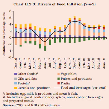

II.2.12 Food inflation in India has undergone diverse movements over the years. With a structural break in December 2013, it has since dropped down to single digit after broadly remaining in double digits for around 20 months. During January 2011 to March 2018, both CPI-cereals inflation and CPI-pulses inflation witnessed two structural breaks, with the onset and spread of monsoon a major factor behind the breaks. Further, the easing phase in recent years in prices of both cereals and pulses is largely driven by cyclical components, indicative of good monsoon, bountiful supply and soothing global food prices.

II.2.13 Prices of perishable items – primarily vegetables – that account for 13 per cent of the food group and 6 per cent of the CPI, were the principal drivers of the rise and fall of food inflation during the year. During 2016-17 and 2017-18, fluctuations in vegetables prices have proved pivotal in determining turning points and amplitude of food price waves, notwithstanding their low weight in the CPI relative to cereals and products. Notably, the trend and cyclical components of CPI-vegetables prices have reversed after the post demonetisation plunge.

II.2.14 Active supply management strategies since November 2017 appear to have played an important role in containing price pressures in vegetables and consequently, in food prices too. In terms of availability of inflation-sensitive vegetables such as tomatoes, onions and potatoes, intra-year movements in prices were influenced by the variability in mandi arrivals.

II.2.15 In the case of prices of tomatoes, inflation went up from (-)41 per cent in June 2017 to 119 per cent in November 2017 due to supply disruptions on account of adverse weather conditions and farmers’ agitations in parts of Maharashtra and Madhya Pradesh. The decline in prices of tomatoes during August-October provided some relief, before the delayed retreat of the monsoon rainfall during October led to crop losses in important tomato producing states like Karnataka, Andhra Pradesh, Telangana, Madhya Pradesh and Odisha. With fresh winter arrivals from December, prices began softening following which tomato inflation dropped to (-)6.6 per cent in March 2018.

II.2.16 Inflation in prices of onions was another shock to food prices during 2017-18. From (-)14 per cent in April 2017, onion price inflation rose to 159 per cent in December. Again, while unfavourable weather was a factor, large procurement of onions by a few state governments was the other principal driver. Post December 2017, onion prices plunged with the arrival of fresh winter crops, supported by supply management measures by the government. The minimum export price (MEP), which is the key supply management measure used by the government to contain upsurges in onion prices, was re-implemented and fine-tuned during the year. This helped bring down onion price inflation to 66.8 per cent in March 2018. In the case of potatoes, delayed sowing in West Bengal – the key growing state in the country – due to extended monsoon showers in October induced price pressures, although carry-over stocks from the previous crop helped to rein them in. A defining characteristic of vegetables price developments in 2017-18 is that while the seasonal softening that usually begins in November was delayed, the cumulative corrections since December have been much more pronounced (Chart II.2.4).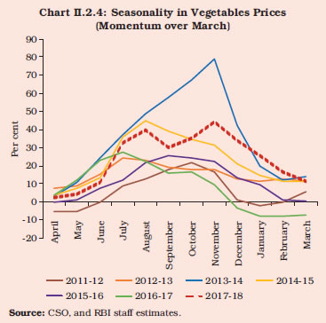

II.2.17 Excluding vegetables, food inflation would have averaged 1.5 per cent during July 2017-March 2018 (as against the actual food inflation of 3.0 per cent) as compared to 5.3 per cent during the same period of 2016-17.

II.2.18 Pulses, with a weight of around 5 per cent in the food group, imposed persistent downward pressures on food inflation throughout the year. This is illustrated by the significant shift in the contribution of prices of pulses to overall inflation from (+)6.0 per cent in 2016-17 to (-)17.9 per cent in 2017-18. With the production of pulses during 2017-18 higher at 24.51 million tonnes (23.13 million tonnes in 2016-17), double-digit deflation in pulses became more pronounced relative to the previous year. Mandi level arhar and urad prices in the major producing states of Maharashtra, Madhya Pradesh, Gujarat, Uttar Pradesh and Karnataka trailed well below their minimum support prices (MSPs), reflecting lower procurement relative to supply. Market prices remain above A2 costs (i.e., production costs excluding imputed labour costs), however, and as a result, adverse supply responses are not yet evident but may be inevitable, going forward. Some mitigating measures have been adopted by the government during the course of the year – removal of the export ban on all pulses, imposition of 60 per cent import duty on gram and 30 per cent import duty on masoor.

II.2.19 Prices of oilseeds, in particular of soyabean, mustard and groundnut, also fell below their MSPs on the back of healthy domestic production during 2017-18 (30.64 million tonnes) on top of a bumper crop in 2016-17 (31.28 million tonnes), after two consecutive years of drought. As a result, the prices of edible oils (mustard and groundnut) also fell and inflation treaded in negative territory for the major part of 2017-18. International prices of edible oils also eased on the back of strong global production, passing through into domestic prices through imports. The government raised the basic customs duties on different edible oils in August 2017, November 2017 and March 2018 to support domestic prices by curbing cheaper imports.

II.2.20 Sugar and spices also contributed to the overall moderation in food inflation with imports improving supply alongside higher domestic production (sugarcane production increased to 35.51 million tonnes in 2017-18 from 30.61 million tonnes in 2016-17). Inflation in cereals generally remained benign during the year, easing in the second half on comfortable stock positions.

Fuel

II.2.21 The fuel group (6.8 per cent weight in the CPI) contributed 11.3 per cent to headline inflation during the year, up from 4.8 per cent a year ago. Fuel inflation picked up from July 2017 and reached a high of 8.2 per cent in November 2017 from an intra-year low of 4.5 per cent in June 2017, before easing to 5.7 per cent in March 2018. The rapid rise was led by prices of LPG and kerosene, reflecting the calibrated increase in their administered prices by the government since July 2016 with the aim of reducing the subsidy and progressively aligning domestic prices with international prices. On the other hand, domestic non-subsidised LPG prices largely tracked international LPG price movements (Chart II.2.5). The average price of non-subsidised LPG cylinders available for four metro cities fell by around ₹57 in March 2018 over December 2017, which was reflected in the moderation in fuel and light inflation during Q4:2017-18. Following the decision of the government to raise kerosene prices by 25 paise per litre every fortnight until the subsidy is eliminated, the gap between international and domestic kerosene prices has narrowed. Firewood and chips was another major contributor to the rise in fuel and light inflation during the year.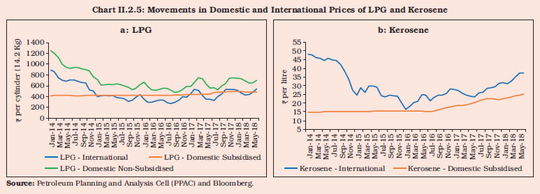

Inflation Excluding Food and Fuel

II.2.22 After remaining sticky through 2016-17, CPI inflation excluding food and fuel reached a low (in the new CPI series) of 3.8 per cent in June 2017, reflecting subdued price pressures and favourable base effects. Since then it has increased steadily till December 2017 and stayed around 5.2 per cent during Q4:2017-18, largely driven by prices of miscellaneous goods and services, and housing, which includes the statistical effect of HRA hikes (Chart II.2.6).

Adjusting for the impact of HRA, annual average inflation in excluding food and fuel group stood lower by around 40 bps at 4.2 per cent during 2017-18.

II.2.23 Net of housing, inflation excluding food and fuel averaged 4.1 per cent in 2017-18, down from 4.7 per cent in the previous year. The increase in HRA for central government employees became effective from July 2017 and its impact on housing inflation peaked in December 2017. This impact has gradually started waning from July 2018 and is expected to fade away fully by December 2018. For policy purposes, more than the direct impact of the HRA hike, a major part of which is purely statistical in nature, the second-round effects through the channel of inflation expectations would require careful monitoring. Moreover, the implementation of HRA by various state governments during 2018-19 could pose an upside risk to the inflation trajectory.

II.2.24 Within the miscellaneous group, inflation in transport and communication prices edged lower during the second half of the year to 2.3 per cent from 3.1 per cent in the first half, mainly on account of cuts in excise duties on retail prices of petrol and diesel by ₹2 per litre in October 2017 and the delayed pass-through of the rise in international crude oil prices during November-December. During 2017-18, price of the Indian basket crude oil reached its intra-year low of USD 46.6 per barrel in June 2017 in line with global crude oil prices. Since then, crude oil prices have increased month-over-month barring February 2018, with an intra-year peak of USD 67.1 per barrel in January 2018 (Chart II.2.7). On an annual average basis, the price of the Indian basket of crude oil increased by 18.5 per cent during 2017-18 (from USD 47.6 per barrel to USD 56.4 per barrel in 2017-18). The pass-through of crude oil prices to petroleum products prices like petrol and diesel picked up in Q4:2017-18 after remaining muted during October-December 2017.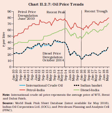

II.2.25 Moderation in prices of communication services – telephone and internet charges – largely reflected increased competition among service providers. Amongst other miscellaneous components, inflation in education prices moderated during the second half of the year, while the remaining components – health, recreation and amusement, household goods and services, and personal care and effects – recorded a pick-up in the second half, partly reflecting hikes in customs duties on items like TV LED panels, mobile handsets, footwear as well as an increase in gold prices.

4. Other Indicators of Inflation

II.2.26 For the year as a whole, sectoral CPI inflation based on Consumer Price Index of Agricultural Labourers (CPI-AL) and Consumer Price Index of Rural Labourers (CPI-RL), which do not have housing components, eased in line with overall CPI inflation, while the inflation in Consumer Price Index of Industrial Workers (CPI-IW) and Consumer Price Index-Combined (CPI-C) converged in January 2018. The housing index under the CPI-IW is adjusted twice a year in January and July (in contrast with the continuous adjustment under CPI-C as a sixth of the sample gets covered every month). Therefore, the impact of the implementation of HRA was reflected in CPI-IW in January 2018.

II.2.27 Inflation measured by the WPI increased, while the GDP deflator based measure decreased during 2017-18. The rise in global crude oil prices, the hardening of metal prices due to the crackdown on polluting industries by China, and strengthening global growth spurred a rise in input costs and contributed to the turnaround in domestic farm and non-farm input costs during 2017-18.

II.2.28 Moderate increases in MSPs were announced during 2017-18 for cereals. Crops such as cotton and coarse grains, particularly bajra and ragi, received major hikes in their MSPs, and the government continued to incentivise the production of pulses and oilseeds by raising their MSPs. The role of MSPs in inflation formation from the cost side hinges on adequate procurement to ensure that market prices remain at or above the announced MSPs and remains a crucial inflation uncertainty for the upcoming year (Box II.2.2).

Box II.2.2 Minimum Support Prices (MSPs) – Do They Influence Inflation Trajectory in India? The role of MSPs in influencing the inflation trajectory in India has been an issue of intense academic and public policy debate. While some studies indicate MSPs to be a major determinant of inflation (Kapur and Behera, 2012), others suggest limited impact (Sonna et al, 2014). There is also a view that MSPs may not have an independent impact on inflation (Lahiri, 2014). A dampening impact of MSPs on inflation due to the associated higher supply response is also highlighted (Gulati and Saini, 2014). While empirical findings are mixed, the announcement by the government in the Union Budget 2018-1912 to fix the MSPs at 1.5 times of cost of farm production effective kharif season 2018 warrants a reassessment of the impact of MSPs on the inflation trajectory. The government announces MSPs for 23 major crops prior to their sowing seasons to ensure guaranteed prices to farmers and protection from price fluctuations and market imperfections. Of these 23 items, 16 can be mapped to the CPI basket. Against this backdrop, a dynamic panel regression model is estimated using Generalised Method of Moments (GMM) in view of the possible problem of endogeneity (i.e., MSPs inducing a positive production response, and higher production requiring lower increases in MSPs) to assess the aggregate impact of MSPs on inflation of the 16 items under the new CPI-C series over the period 2011-12 to 2017-18: where, Y14,16;t is weighted CPI of the 14 or 16 MSP items in period t, as the case may be; Y(14,16;t–1) is the weighted CPI with one period lag, Xi,t are individual MSPs of the 14 or 16 crops in period t; and Zi,t is individual production of the 14 or 16 crops in period t. The estimation uses several instrumental variables, e.g., agricultural wages, yields, lagged MSP, lagged production, procurement (of rice and wheat) and a rain dummy defined as deviation of south west monsoon from normal by +/-5% and the north east monsoon by +/-15%. The model is estimated under three scenarios: (i) for all the 16 CPI items with procurement as an instrumental variable (Scenario I), (ii) for all the 16 CPI items without procurement as an instrumental variable (Scenario II), and (iii) for 14 CPI items, i.e., by dropping rice and wheat (where procurement is maximum at about 35 per cent of output) from the panel (Scenario III)13. The findings suggest that MSPs have the maximum impact on 16 items within the CPI food basket. The coefficients on the MSP term indicate that the impact of change in MSP on inflation is estimated to be stronger when procurement is used as an instrumental variable (Scenario I) than without (Scenario II). In contrast, excluding rice and wheat from the panel (i.e., in the case of CPI 14), the MSP impact on inflation becomes statistically insignificant (Scenario III). This suggests that adequate procurement is the channel through which higher MSPs may push up the food inflation trajectory (Table 1). Table 1: Empirical Results of the Dynamic Panel Data Model (16 Crops with MSP; 2011-12 to 2017-18) Explanatory Variables Scenario – I (CPI16 With Procurement IV) Scenario – II (CPI16 Without Procurement IV) Scenario – III (CPI14 Without Procurement IV) 1 2 3 4 log (Food.CPI16)(–1) 0.52 (23.33)*** 0.54 (54.28)*** --- log (Food.CPI14)(–1) --- --- 0.83 (10.99)*** log (MSP16) 0.16 (6.61)*** 0.13 (16.50)*** --- log (MSP14) --- --- -0.06 (-0.49)# log (Production16) -0.04 (-5.01)*** -0.02 (-6.55)*** --- log (Production14) --- --- -0.17 (-4.59)*** Diagnostics       J-Statistics/prob (J-stats) 11.46; 0.12 13.19; 0.15 6.32; 0.38 Arellano-Bond test for AR(1) in first differences z/prob (z) -2.88; 0.001 -3.33; 0.00 -2.08; 0.04 Arellano-Bond test for AR(2) in first differences z/prob (z) -0.38; 0.701 1.21; 0.23 -0.26; 0.79 Notes: 1. MSP14 and CPI14 are excluding rice and wheat. 2. Figures in parentheses are t-statistics. 3. ***: Significant at 1%; #: Insignificant. Instrumental variables (IV): Log(AgriWage)(0); log(P.Yield)(0); log(MSP)(-1,2,3); Raindummy; log(area); log(procurement); log(Production)(-1,2) Source: RBI staff estimates. The hypothesis is also examined for individual crops over the period 2008-09 to 2017-18 by studying the heterogeneity in production and procurement across states in a panel framework. Accordingly, the retail price of a crop in a state is modelled as a function of MSP, production, procurement and international prices, i.e., the information that enters into fixation of MSPs by the Commission for Agricultural Costs and Prices (CACP). International prices and lagged retail prices are used as control variables. The problem of simultaneity bias (between MSP and retail prices) is addressed by the pre-announced nature of MSPs, while the inclusion of lagged retail prices and international prices alleviates omitted variable bias (as MSPs respond to these prices). Thus, the baseline specification of retail prices of individual crops is as follows: The results of the baseline model are presented in Table 2. They show that MSP has a positive and statistically significant effect on retail prices of all crops, although it varies significantly across crops. In general, it has a stronger effect for those crops where procurement is substantial, such as paddy and wheat. Additionally, the control variables throw up some interesting results: while international prices play a stronger role in determining edible oil prices, production dampens prices the most in the case of pulses; pulses prices also exhibit the highest persistence among all crops; higher procurement in paddy is associated with lower prices, perhaps indicating a situation of over-supply. Table 2: Annual Data Panel Regressions Dependent Variable log (Retail Price) (1) (2) (3) (4) (5) (6) (7) (8) (9) (10) (11) (12)   Rice Wheat Arhar Urad Moong Gram Masoor Groundnut Soyabean Rapeseed Sunflower log (MSP) 0.91*** 1.27*** 0.44*** 0.15*** 0.14*** 1.13*** 0.64*** 0.57*** 0.60*** 0.83*** 0.61***   (0.10) (0.08) (0.10) (0.04) (0.03) (0.06) (0.06) (0.13) (0.08) (0.08) (0.06) log (International Price) 0.07 0.03           0.40*** 0.44*** 0.48*** 0.63***   (0.09) (0.02)           (0.05) (0.02) (0.04) (0.07) log (Production) -0.02 -0.20* -0.29     -0.30*** -0.08 -0.07* -0.01 -0.07 -0.05**   (0.07) (0.08) (0.16)     (0.05) (0.07) (0.03) (0.03) (0.10) (0.01) log (Procurement) -0.10** 0.002                     (0.03) (0.01)                   log (Retail Price)(-1) 0.20 0.06 0.60*** 0.45*** 0.31*** 0.01 0.90*** -0.02 0.004 -0.06 0.16***   (0.12) (0.07) (0.05) (0.03) (0.04) (0.07) (0.05) (0.15) (0.13) (0.10) (0.04) Constant -4.31*** -6.29*** -2.25* 1.19*** 1.91*** -5.39*** -4.73*** -2.84*** -3.31*** -5.11*** -5.58***   (0.80) (0.43) (0.97) (0.22) (0.22) (0.26) (0.64) (0.75) (0.31) (0.39) (0.71) Observations 57 48 60 207 209 82 36 48 27 61 40 Notes: 1. *: p<0.05 **: p<0.01 ***: p<0.001. 2. Standard errors in parentheses. Source: RBI staff estimates. Thus, both the panel studies (from a historical perspective), suggest a statistically significant impact of MSPs on retail inflation in the presence of adequate procurement. The actual impact of the MSP hike for 2018-19 kharif season, however, would depend on the procurement strategy of the government as well as the ruling market prices of various crops vis-à-vis the revised MSPs. References: 1. Gulati, A. and S. Saini (2014), “Food Inflation in India - Diagnosis and Remedies”, ed. Uma Kapila (Indian Economy since Independence: Academic Foundation, 2014). 2. Kapur, M. and H. Behera (2012), “Monetary Transmission Mechanism in India: A Quarterly Model”, RBI Working Paper Series, WPS (DEPR): 09/2012. 3. Lahiri, A. (2014), “Don’t blame MSP for inflation’’, The Indian Express, October. 4. Sonna, T., H. Joshi, A. Sebastian, and U. Sharma (2014), “Analytics of Food Inflation in India”, RBI Working Paper Series, WPS (DEPR): 10/2014.

II.2.29 Growth in nominal rural wages, both for agricultural and non-agricultural labourers, generally moderated from August 2017, partly reflecting the lagged effects of softer inflation. A survey conducted during August-September 2016 in six Indian states, viz., Gujarat, Kerala, Odisha, Punjab, Uttar Pradesh and West Bengal, shows that casual labour households are more likely to secure work under the Mahatma Gandhi National Rural Employment Guarantee Scheme (MGNREGS), which can potentially lead to a shortage of labour and upward pressure on wages (Box II.2.3). In the case of the corporate sector, staff costs have exhibited high sensitivity to inflation expectations of households, pointing to the importance of anchoring inflation expectations in order to minimise the risk of a wage-price spiral.

Box II.2.3 Impact of MGNREGS on Rural Labour Market: An Assessment Using Survey Data The need for strengthening social safety nets has been a key feature of public policy across the globe. In this context, India’s Mahatma Gandhi National Rural Employment Guarantee Scheme (MGNREGS) launched under the MGNREG Act, 2005 has been ranked as the world’s largest public works programme, providing a social security net to almost 15 per cent of the country’s population (World Bank, 2015). Its bottom-up, peoplecentred, demand-driven, self-selecting, rights-based design is innovative and unprecedented. However, while the scheme aims to provide 100 days of employment, the average employment provided remained below 50 days at the all-India level with marked divergence across states (Chart 1). Furthermore, there are discernible differences in implementation of the scheme across states. Two states i.e., Tamil Nadu and West Bengal, accounted for nearly one-fourth of employment provided through MGNREGS, which was more than their share in total rural households. Maharashtra and Bihar, which have a higher share in total rural households, generated comparatively lower employment through MGNREGS (Chart 2). Against this backdrop, a primary survey was carried out among MGNREGS workers with a total sample of 1,798 during August-September 2016 in select six Indian states with diverse economic and labour market conditions.The states were Gujarat, Kerala, Odisha, Punjab, Uttar Pradesh and West Bengal, covering eastern, western, northern and southern parts of the country to get a holistic view on the impact of MGNREGS on wage level and labour market participation. 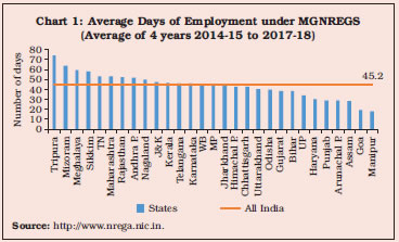The survey revealed that more than half of the respondents were otherwise unemployed in Kerala, Gujarat and Punjab, while in Uttar Pradesh, Odisha and West Bengal, they were largely employed as agricultural labourers. The survey results also showed that (i) in all the surveyed states, only a few avoided MGNREGS work for alternate employment, and (ii) the avoidance of traditional labour for MGNREGS was different across states and across labour groups. The shift to MGNREGS from traditional employment is more in case of casual labour households and is more evident in Odisha (75 per cent), Uttar Pradesh (66 per cent) and West Bengal (42.5 per cent) rather than Punjab (29.6 per cent), Kerala (24.1 per cent) and Gujarat (8.3 per cent). For the analysis, avoidance of traditional employment for MGNREGS was taken as the dependent variable. Given the dichotomous dependent variable, a non-linear regression model was used. Heckman’s sample selection model was applied to address the likely specification bias in the model. The ρ value and Wald statistic in the Heckman model turned out to be insignificant, indicating absence of correlation between error terms of selection and outcome equations. Accordingly, a probit model was used for estimating the regression taking only the respondents who are employed other than under MGNREGS. The dependent variable takes the value 1 when the respondents shift from traditional employment to MGNREGS and zero otherwise; where, yi – whether avoided alternate employment for MGNREGS: Yes=1 and No=0; CLA – casual labour of agriculture: Yes=1 and No=0; CLNA – casual labour of non-agriculture: Yes=1 and No=0; G – Gender: Female=1 and Male=0; P – poverty measured in terms of ration card status: BPL/Antyodaya/Annapurna=1 and APL=0; W=square of wage difference between wages from other employment and MGNREGS wages; M=number of earning members in the family; and C – Caste: Scheduled Caste/ Scheduled Tribe=1 and Others=0. 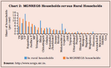The coefficients of the probit model show the direction of relationship while the marginal effects (dy/dx column in Table 1) give the partial effect of each explanatory variable on the probability that the observed dependent variable yi = 1, in this case the probability of avoiding traditional work for MGNREGS. The results show that for a casual labourer in agriculture, the probability of avoiding traditional work increases by 19 per cent, while in the non-agriculture casual labour category, this is 11 per cent. The difference in wages (actual minus MGNREGS) was significant with a negative relationship (the probability impact of this is small at 0.0003 per cent). This shows that greater the difference in wages between traditional and MGNREGS employment, lower the probability of avoiding traditional work for the latter. Thus, casual labourers are more inclined to avoid traditional employment for MGNREGS and the difference in wages is a significant factor in this decision (Table 1). Table 1: Results of Probit Model – Average Marginal Effects Variables dy/dx Std. Err. z Number of observations = 968 Model VCE: Robust Probability [95% Conf. Interval] Casual labour in agriculture 0.19 0.03 6.23 0.001 0.13 0.25 Casual labour in non-agriculture 0.11 0.04 2.89 0.004 0.04 0.19 Difference in wages -.000003 0.000001 -3.36 0.001 -0.000005 - 0.000001 Caste 0.03 0.03 0.93 0.351 -0.03 0.09 Gender -0.01 0.03 -0.23 0.818 -0.07 0.06 Poverty 0.03 0.04 0.73 0.463 -0.04 0.09 No. of earning members 0.002 0.01 0.12 0.906 -0.03 0.03 Note: Wald chi2(7) = 62.77; Prob > chi2 = 0.0000. Log pseudolikelihood = -614.31906; Pseudo R2 = 0.0500. Source: RBI staff estimates. However, the limited number of employment days provided under the scheme has restricted the impact on the labour market as a whole. If and when the scheme is implemented fully, it has the potential to create shortages in labour supply in the casual labour category, propelling a wage increase in this segment. However, if the scheme is designed judiciously so as to provide employment during off seasons, it can be complementary to traditional employment by offering a fall back option. Such complementarities were evident in West Bengal to the extent that the work schedule was adjusted to the seasonality of traditional employment. References: 1. http://www.nrega.nic.in. 2. World Bank (2015), “The State of Social Safety Nets 2015”.

5. Concluding Observations

II.2.30 In sum, the inflation path altered dramatically over three phases during 2017-18, highlighting how quickly inflationary pressures can get generalised and pose policy challenges. The current inflation outlook is clouded by several uncertainties. First, the staggered impact of HRA increases by various state governments may push up headline inflation in 2018-19, and potentially induce second-round effects. Second, a pick-up in global growth and/or geopolitical risks may exert further pressure on crude oil and commodity prices, with implications for domestic inflation. Third, at this stage, there is considerable uncertainty about the full impact of the MSPs for kharif crops on inflation. Fourth, volatility in global financial markets continues to impart uncertainty to the inflation outlook. Finally, the strengthening of the growth momentum could also exert demand pull pressures, unless the supply response is proportionate and timely. On the downside, the recent pick-up in monsoon, after the initial lull, in conjunction with comfortable carry-over stocks from the current year on the back of record foodgrains production could help in containing food price pressures. Trade/tariff wars could end up being a drag on the global recovery and moderate inflation by weakening aggregate demand. Overall, there is a need for vigilance around the evolving inflation scenario in the coming months of the year.

II.3 MONEY AND CREDIT

II.3.1 During H2:2017-18, monetary and credit indicators rebounded from the effects of demonetisation. Money supply (M3) was driven up by scheduled commercial banks’ (SCBs’) credit growth, which witnessed a revival from its historic low in March 2017 and re-emerged as a significant source of financing for the commercial sector.

II.3.2 Against this backdrop, the immediately following sub-section on reserve money (RM) brings to the fore, the sustained dominance of foreign exchange assets as the largest source of RM during the year. The follow-up section on M3 documents the contrasting variations between H1 and H2 of 2017-18 as the effects of demonetisation waned; it also addresses cryptocurrency developments in the global and Indian context. The turnaround in credit in 2017-18 is investigated at both macro and sectoral levels in sub-section 3 with implications for the aggregate resource flow to the commercial sector.

1. Reserve Money

II.3.3 During 2017-18, the evolution of RM — a stylised depiction of the Reserve Bank’s balance sheet that focuses on ‘moneyness’¹⁴ — was primarily conditioned by the remonetisation of currency in circulation with newly designed notes of denomination of ₹10, ₹50, ₹200, ₹500 and ₹2000. The impact of demonetisation had plunged RM growth into contraction till November 10, 2017. Between November 9, 2016 – the effective date of demonetisation – and December 31, 2016, the Reserve Bank pumped in 23.8 billion pieces of banknotes into circulation aggregating ₹5,540 billion in value. Keeping in view the urgent need to make available adequate cash to all parts of the country at the shortest possible time, concerted efforts were made by the Reserve Bank and the printing presses to augment the production and supply of new banknotes. In Q1:2017-18, remonetisation efforts shifted into overdrive to engineer a quick recovery from the shock of demonetisation. In the ensuing months, favourable base effects kicked in and RM growth surged to an all-time peak of 60.6 per cent on January 5, 2018 before moderating to around 27 per cent as on March 31, 2018. RM growth was 21.1 per cent as on June 29, 2018.

II.3.4 Currency in circulation (CiC), the major driver of RM, increased by around ₹4.9 trillion on a year-on-year basis. While the CiC as on March 31, 2018 accounted for 101.8 per cent of its pre-demonetisation level, it works out to around 88 per cent of its underlying 3-year trend had there been no demonetisation (Chart II.3.1). Consequently, India’s currency to GDP ratio moved up to 10.9 per cent in 2017-18, returning to being amongst the highest levels of currency usage in peer emerging market economies (EMEs) and advanced economies (AEs) as well (Appendix Table 4). In consonance, the use of digital payments¹⁵, which had surged to a peak in December 2016 in the aftermath of demonetisation fell back to the elevated post-demonetisation trend before rising in recent months.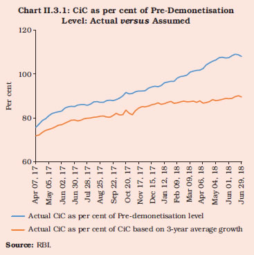

II.3.5 Amongst other components of RM, bankers’ balances with the Reserve Bank grew at a moderate pace, reflecting the deceleration in bank deposits during the year. Banks’ average daily cash balances, nonetheless, turned out to be 101.1 per cent of the cash reserve ratio (CRR) prescription, with the demand for excess reserves moderated by the persistence of surplus liquidity conditions throughout the year, barring the episodes of tightness in Q4:2017-18 (Chart II.3.2).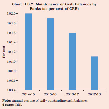

II.3.6 Turning to the sources, net foreign exchange assets of the Reserve Bank rose to account for 114.1 per cent of RM on March 31, 2018, up from the preceding 5-year average of around 110 per cent (Chart II.3.3). The consequent injection of liquidity of ₹2.2 trillion trebled over its level in the previous year. Among other sources, net credit to the government sector declined by around 23.3 per cent due to open market sales by the Reserve Bank as well as higher central government deposits. In addition, average liquidity adjustment facility (LAF) reverse repo (average of outstanding on each Friday) increased to ₹2.2 trillion in 2017-18 from ₹1.5 trillion a year ago, reflecting de facto excess reserves due to the surge in deposits following demonetisation in 2016-17 and low credit offtake till H1:2017-18. With the gradual increase in CiC, the absorption of liquidity through open market operation (OMO) sales beginning July 2017 and the improvement in credit offtake from November 2017, the liquidity position reversed and LAF absorption gave way to a net repo of ₹575 billion as on March 31, 2018 (net reverse repo of ₹3.1 trillion a year ago).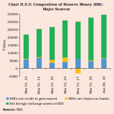

II.3.7 Higher expenditure by the centre and lower revenues relative to budget estimates in H1:2017-18 led to frequent recourse to ways and means advances (WMA) from the Reserve Bank, thereby adding to surplus liquidity with the banking system. Consequently, large amounts parked under reverse repo despite absorption through Market Stabilisation Scheme (MSS) T-Bills, OMO sales and the increase in CiC impacted monetary aggregates. Subsequent to advance tax inflows in September 2017, government expenditure moderated, which was reflected in a gradual decline in net reverse repo (Chart II.3.4). With the introduction of a standing deposit facility, the Reserve Bank will have a new tool to absorb liquidity without collateral constraints (Box II.3.1).

2. Money Supply

II.3.8 Movements in money supply (M3) during 2017-18 reflected shifts in the Reserve Bank’s balance sheet encapsulated in changes in RM in the preceding section as well as broader developments in the economy that impacted banks’ balance sheets. In H1, the lingering effects of demonetisation weighed heavily on currency with the public (CwP) which remained in contraction mode. Moreover, deposit growth slowed sharply after the post-demonetisation bulge of the preceding half and also reflected the pronounced deceleration in domestic economic activity in Q1:2017-18. Consequently, the growth of M3 slumped on a year-on-year basis to reach a historic low of 5.6 per cent as on September 29, 2017. In H2, however, the tide turned and the rapid pace of remonetisation finally lifted the growth in currency with the public (CwP) into positive territory. The growth of M3 recovered and assumed an upward trajectory, crossing into double digit on December 22, 2017. It stood at 9.2 per cent as on March 31, 2018, up from 6.9 per cent a year ago. M3 growth stood at 9.8 per cent as on June 22, 2018 (Table II.3.1).

II.3.9 The behaviour of M3 essentially mirrored its recently turned volatile component – CwP – which accounted for 12.6 per cent of M3 as on March 31, 2018. As stated earlier, growth in CwP remained in negative territory in H1:2017-18 but turned positive for the first time after a gap of almost one year on November 10, 2017 and rose by 39.2 per cent by March 31, 2018, a sharp contrast with the contraction of 20.8 per cent a year ago. As on June 22, 2018, CwP growth was 29.2 per cent (a decline of 12.6 per cent during the corresponding fortnight last year).

II.3.10 Aggregate deposits accounted for around 93 per cent of M3 following their sharp increase in Q3 of 2016-17 due to substitution of CwP by deposits in the post-demonetisation phase. With the phase-out of restrictions on cash withdrawals and the gradual pick-up in currency demand, deposit growth started decelerating and reached its lowest level of 2.6 per cent on December 8, 2017. Over the rest of the year, deposit growth increased steadily, but at 5.8 per cent on March 31, 2018 it was sizably lower than 11.1 per cent a year ago. Both demand deposits and time deposits shared this moderation as the interest rate on deposits eased, with banks transmitting the cumulative reduction of 200 bps in the policy rate by the Reserve Bank almost fully to term deposit rates. This resulted in the returns on deposits turning less attractive relative to competing financial instruments, particularly mutual funds. This disintermediation impacted deposit behaviour significantly. The combination of surplus liquidity conditions in the wake of demonetisation and lower offtake of credit consequent upon slower economic activity also worked to mute the expansion of deposits in H1.

II.3.11 The public disenchantment from lower returns from bank deposits coupled with sobering down of returns from other assets was followed by an interesting development. Cryptocurrencies came under focus globally as an alternative source of high returns albeit with a high risk element (Box II.3.2).

Box II.3.2 Cryptocurrency: Evolving Challenges Cryptocurrency is a class of privately issued digital means of payment that depends predominantly on cryptography and distributed ledger technology (DLT) such as the blockchain. A blockchain is a continuous ledger in which transactions are stored as blocks and linked using cryptography. Cryptocurrency is often allotted through initial coin offerings (ICOs), which are used as a means of raising capital through crowdfunding. Cryptocurrency typically has some monetary characteristics, but is not a liability of any entity and is not backed by any authority. Its value is driven by users’ confidence in it. This, coupled with limited supply, makes its value highly volatile and, therefore, not a reliable medium of exchange or store of value (Chart 1). Though cryptocurrency may not currently pose systemic risks, its increasing popularity leading to price bubbles raises serious concerns for consumer and investor protection, and market integrity. Notably, Bitcoins lost nearly US$200 billion in market capitalisation in about two months from the peak value in December 2017. As per the CoinMarketCap, the overall cryptocurrency market had nearly touched US$800 billion in January 2018. The cryptocurrency eco-system may affect the existing payment and settlement system which could, in turn, influence the transmission of monetary policy. Furthermore, being stored in digital/electronic media – electronic wallets – it is prone to hacking and operational risk, a few instances of which have already been observed globally. There is no established framework for recourse to customer problems/ disputes resolution as payments by cryptocurrencies take place on a peer-to-peer basis without an authorised central agency which regulates such payments. There exists a high possibility of its usage for illicit activities, including tax avoidance. The absence of information on counterparties in such peer-to-peer anonymous/pseudonymous systems could subject users to unintentional breaches of anti-money laundering laws (AML) as well as laws for combating the financing of terrorism (CFT) (Committee on Payments and Market Infrastructures – CPMI, 2015). The Bank for International Settlements (BIS) has recently warned that the emergence of cryptocurrencies has become a combination of a bubble, a Ponzi scheme and an environmental disaster, and calls for policy responses (BIS, 2018). The Financial Action Task Force (FATF) has also observed that cryptoassets are being used for money laundering and terrorist financing. A globally coordinated approach is necessary to prevent abuses and to strictly limit interconnections with regulated financial institutions. 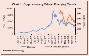On a global level, regulatory responses to cryptocurrency have ranged from a complete clamp down in some jurisdictions to a comparatively ‘light touch regulatory approach’. The Securities and Exchange Commission (SEC) and the Commodity Futures Trading Commission (CFTC) have emerged as the primary regulators of cryptocurrencies in the United States, where these assets like most other jurisdictions, do not enjoy the legal tender status. Asian countries have experienced oversized concentration of crypto players – Japan and South Korea account for the biggest shares of crypto asset markets in the world. In the case of Bitcoins, half of transactions worldwide are carried out in Japan. In September 2017, Japan approved transactions by its exchanges in cryptocurrencies. China’s exchanges hosted a disproportionately large volumes of global Bitcoin trading until their ban recently. In India, the government and the Reserve Bank are keeping a close watch on cryptocurrency and have issued pre-emptive cautionary warnings. In early April 2018, the Reserve Bank barred its regulated entities from dealing in or providing services to any individual or business entities dealing with or settling in virtual currencies. Regulated entities which already provide such services were asked to exit the relationship within three months. Developments on this front need to be monitored as some trading may shift from exchanges to peer-to-peer mode, which may also involve increased usage of cash. Possibilities of migration of crypto exchange houses to dark pools/cash and to offshore locations, thus raising concerns on AML/CFT and taxation issues, require close watch. Unlike the concerns on privately issued cryptocurrency, the adoption of DLT in the domain of payment, clearing and settlement solutions holds the promise of significant economic benefits in future. Rapid changes in the landscape of the payments industry, along with factors such as emergence of private digital tokens and the rising costs of managing fiat paper/metallic money, have led central banks around the world to explore the option of introducing fiat digital currencies. In India, an inter-departmental group has been constituted by the Reserve Bank to study and provide guidance on the desirability and feasibility to introduce a central bank digital currency. References: 1. BIS (2018), “Annual Economic Report”, June, Basel. 2. CPMI (2015), “Digital Currencies”, November.

II.3.12 From the sources side, bank credit to the commercial sector was the key mover of M3 in 2017-18, accounting for 68.5 per cent of the change in M3 during the year, followed by net foreign exchange assets of the banking sector (Chart II.3.5).

II.3.13 The expansion in bank credit to the commercial sector was more pronounced during H2 of 2017-18. This needs to be seen in conjunction with an expansion in net bank credit to government at a slower pace.

II.3.14 During the year, monetary ratios such as the currency-deposit (C/D) ratio and the money multiplier (MM) exhibited behaviour in contrast to the pattern observed in the previous year. The C/D ratio experienced a steep rise due to expansion in CwP and moderation in aggregate deposits. The MM, which rose to a peak of 8.8 on January 6, 2017, started declining gradually with the process of remonetisation. As on June 22, 2018, MM stood at 5.6 vis-à-vis 6.3 a year ago. Adjusted for reverse repo (net) with banks - analytically akin to banks’ deposits with the central bank – the MM would turn out to be slightly higher at 5.8 as on June 22, 2018 vis-à-vis 5.5 a year ago. However, the reserve-deposit (R/D) ratio remained broadly stable, reflecting the unchanged CRR during the year (Chart II.3.6).

3. Credit

II.3.15 The growth in SCBs’ credit started decelerating from November 2016 and reached an all-time low of 3.7 per cent on March 3, 2017. Although credit growth recovered in the subsequent fortnights, it trailed well below its trajectory in the previous year through April-October 2017. Besides the aftershock of demonetisation, weak demand for new bank financing and deleveraging by banks struggling with provisions for mounting loan delinquency also took their toll. Non-banks replaced bank credit as sources of funding for the commercial sector during this phase. From November 10, 2017, credit growth picked up as the quickening of economic activity spurred a hesitant recovery and levels of non-performing assets started plateauing albeit at elevated levels. By December 22, 2017, credit growth touched double digit – 10.3 per cent for the first time since September 30, 2016. As on March 31, 2018, credit growth stood at 10.0 per cent significantly higher than 4.5 per cent last year. SCBs’ credit growth stood at 12.8 per cent as on June 22, 2018 (5.6 per cent during the corresponding fortnight in the previous year).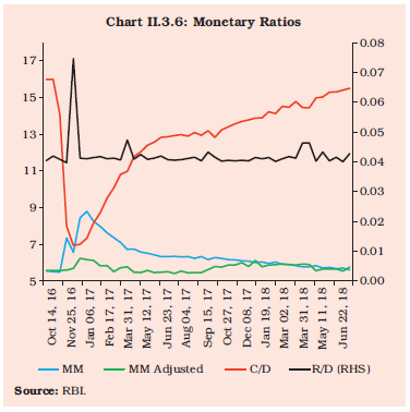

II.3.16 The recovery in credit growth from November 2017 onwards benefited mainly from a favourable base effect as credit levels a year ago were dampened by demonetisation effects. Nonetheless, momentum also provided tailwinds, indicating an upswing in credit in tune with gradually improving domestic demand conditions (Chart II.3.7). However, the credit to GDP gap continued to be negative through 2017-18, implying that actual credit demand remained lower than its potential.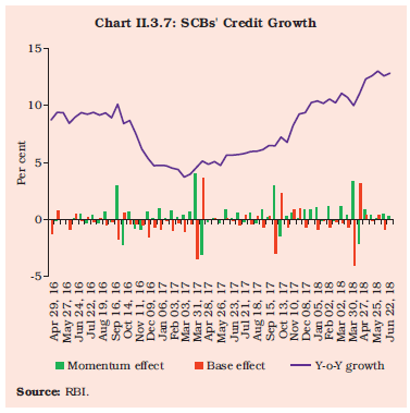

II.3.17 Non-food credit growth accelerated to 10.2 per cent by March 2018 from 5.2 per cent a year ago. Bank loans to industry picked up slowly on a brightening outlook. Shifts into bank credit were also incentivised by the tightening of financing conditions in respect of non-bank sources of finance on account of the hardening of bond yields from October 2017 onwards. Credit growth was largely driven by private sector banks, which were resilient in the face of these tectonic shifts, with their credit portfolio growing at 18.7 per cent during the year as compared to 5.3 per cent by public sector banks (PSBs) and 3.8 per cent by foreign banks. Among PSBs, those under prompt corrective action (PCA) turned out to be laggards, though signs of revival were evident in this category as well during 2018-19 so far (Chart II.3.8). During Q1:2018-19, non-food credit has maintained its momentum, with credit accelerating to 12.9 per cent as on June 22, 2018 as compared to a meagre 6.3 per cent a year ago.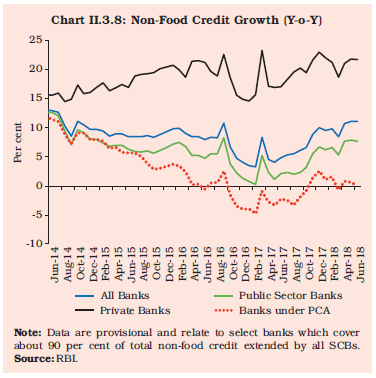

Sectoral Credit Deployment by Banks

II.3.18 The growth in credit to agriculture decelerated during 2017-18 when compared to a year ago. This might be indicative of pressures in the farm sector as corroborated by agriculture debt waivers announced in some states. Credit to industry turned around from a contraction of 1.9 per cent in March 2017 to a positive 0.7 per cent in March 2018 (Table II.3.2). Industrial credit, which had shrunk for most part of 2017-18, recovered from November 2017 onwards. A pick-up was witnessed across sectors such as textiles; vehicles, vehicle parts and transport equipment; engineering; food processing; and rubber, plastic and products. In contrast, credit to infrastructure, which accounted for about one-third of bank credit to industry, contracted in a broad-based manner (by 1.7 per cent in March 2018), pulled down by power, telecommunications and roads. The modest signs of recovery in infrastructure vis-à-vis the previous year's position suggest that the power sector could benefit from improved electricity supply following better availability of coal. The base metal segment remained in stress, despite the recovery in global metal prices. The recent revival in manufacturing activity has provided some boost to base metal prices. The steel segment has improved on strong export demand and revival of domestic activity.

II.3.19 The growth in credit to services decelerated, led by segments like trade and professional services. The personal loans segment recorded acceleration and ran above trend, driven by housing and vehicle loans. Credit card outstanding – a small component in overall credit – recorded deceleration given its high base as also due to sluggishness in demand for consumer durables. Education loans contracted, indicative of aversion of banks in respect of lending to riskier sectors.

II.3.20 All major sectors, barring agriculture, witnessed an acceleration in June 2018. Credit to major sub-sectors such as textiles, engineering, food processing, chemical and chemical products and cement and cement products accelerated. However, credit to basic metal and metal products, construction and gems and jewellery contracted/declined. Services witnessed a sharp surge driven by trade and non-banking financial companies (NBFCs) (Table II.3.2).

Resource Flow to the Commercial Sector

II.3.21 The total flow of financial resources to the commercial sector increased by 27.1 per cent during 2017-18 as compared to an increase of 3.8 per cent in the previous year. While non-food bank credit flows more than doubled to ₹7,959 billion, the resource flow from non-banks decreased by 2.8 per cent, mainly on account of the decline in gross private placements by non-financial entities, sharp fall in commercial paper (CP) issuances and lower credit disbursement by systemically important non-deposit taking NBFCs. The hardening of corporate bond yields in H2: 2017-18 led to lesser issuances of corporate bonds, bringing down mobilisation through this route. However, there was a significant increase in public issuance of equities by non-financial entities, credit disbursement by housing finance companies and accommodation by four All India Financial Institutions (AIFIs) regulated by the Reserve Bank. Among foreign sources, external commercial borrowings (ECB)/foreign currency convertible bonds (FCCB) recorded net outflows for the third consecutive year albeit of a much lower magnitude during the year. Foreign direct investment (FDI) flows declined by 10.3 per cent during the year, mainly due to higher repatriation in the second half of the year (Table II.3.3). Short-term credit from abroad, however, more than doubled to ₹896 billion during the year as import growth accelerated.

II.3.22 In summary, while key monetary and credit aggregates picked up on signs of stronger economic activity in the second half of 2017-18, they remained muted in relation to their historical record. Credit conditions remained tight for the major part of the year as the Reserve Bank’s liquidity operations steadily drained away surplus liquidity and bond yields hardened in response to perceptions of higher supply of government papers, higher than budgeted fiscal deficit numbers and some uncertainty around the inflation outlook. Although credit to industry, and in particular infrastructure, remained subdued, signs of a gradual revival in the second half of the year augur well for the medium-term outlook. Credit to services and personal loans remained resilient during the year. Non-bank sources of credit played an important role, especially domestic sources thereof.

II.4 FINANCIAL MARKETS

II.4.1 Barring the sell-offs in equities and bonds in February and March 2018 that ricocheted across the world, including in India, global financial markets remained generally upbeat in 2017-18 on improving growth prospects and a gradual pace of normalisation by the US Fed. Valuations rose through the greater part of the year amidst subdued volatility, except for brief flares. Fears in February 2018 about a faster pace of policy normalisation by the US Fed on the arrival of strong jobs/wages data and again in March 2018 in response to US trade policies, clouded the outlook as volatility returned amidst considerable flux in asset prices and capital flows with implications for emerging markets. Currencies were boosted by the generally weak US dollar over the greater part of the year, interrupted by idiosyncratic but short-lived reversals on safe haven effects.

II.4.2 In India, global spillovers impacted equity and currency markets the most, puncturing the robust rallies that drove up the former segment right up to February, and reversing the appreciating bias with which the Indian rupee was trading against major currencies over most part of the year. By contrast, other market segments were mostly influenced by domestic factors. In the money market, as discussed in sub-section 1, money market rates remained anchored to the policy rate due to active liquidity management by the Reserve Bank. Sub-section 2 depicts developments in the domestic bond market where yields hardened on inflation prospects, fears of excessive issuances of papers relative to absorption capacity, fiscal slippages, rising crude oil prices and sharp increase in the US bond yields. Developments in the corporate debt market, where yields hardened significantly in H2 after softening initially in H1, have been discussed in sub-section 3. Sub-section 4 portrays developments in the domestic stock market, which remained buoyant on the back of positive domestic factors and cues from global markets. The two-way movements in the Indian rupee-US dollar (INR-US$) exchange rate, generally appreciating in H1 on significant foreign portfolio investment (FPI) inflows but depreciating in H2 on general strengthening of the US dollar and FPI outflows, have been discussed in sub-section 5.

1. Money Market

II.4.3 The money market remained broadly stable during 2017-18, with the Reserve Bank actively managing the post-demonetisation surplus liquidity through reverse repo operations of various tenors, supplemented by outright operations including Treasury Bill (T-Bill) auctions under the market stabilisation scheme (MSS). However, the Reserve Bank conducted variable rate term repo auctions of different tenors to address additional demand for liquidity that is usually observed in March every year. During Q1 of 2018-19, the liquidity condition generally remained in surplus mode mainly reflecting increased government spending. The Reserve Bank actively managed the frictional and structural liquidity conditions with term repos/reverse repos and open market operations (OMOs).

II.4.4 The weighted average call rate (WACR) in the uncollateralised inter-bank call money market traded with a downward bias relative to the policy rate through the year, although the negative spread generally narrowed from 32 basis points (bps) in April 2017 to 5 bps in March 2018 (Chart II.4.1). It may be mentioned that this decline in the negative spread over the policy rate reflected the narrowing of the spread in respect of both ‘traded deals’, which are the call money deals directly transacted on the electronic, negotiated and quote-driven platform for trading, the NDS-CALL and ‘reported deals’ which are over-the-counter (OTC) call deals subsequently reported on the NDS-CALL platform. However, reported deals recorded larger negative spreads over the policy rate vis-à-vis the traded deals. During Q1 of 2018-19, the negative spread of the WACR over the policy rate averaged around 10 bps.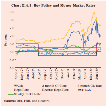

II.4.5 Even as spreads narrowed, volatility in the call money segment, measured by conditional variance, ebbed and turnover remained broadly unchanged. In 2017-18, call transactions constituted less than 10 per cent of the total money market volume.

II.4.6 Collateralised money market instruments are the Collateralised Borrowing and Lending Obligation (CBLO) and market repo. In the CBLO segment, banks are usually the major borrowers, while mutual funds (MFs) are the major lenders. In the market repo segment, however, banks are the major players both on the borrowing and the lending sides; the other participants being Primary Dealers (PDs) mainly as borrowers (with a share of 28 per cent) and mutual funds as lenders (with a share of 30 per cent). Trading volumes and rates in the CBLO segment decline sharply on reporting Fridays with corresponding increases in the market repo segment. This is because borrowings in the market repo segment are exempted from the cash reserve ratio (CRR) requirement, whereas borrowings in the CBLO market are not.

II.4.7 Average daily volume in the money market (call money, CBLO and market repo) increased by 17 per cent to ₹1,687 billion during 2017-18 from ₹1,441 billion in 2016-17. Volumes in the CBLO and market repo segments increased by 25 per cent and 10 per cent, respectively, whereas in the call money segment, they decreased by 8 per cent during the year. Call money, CBLO and market repo segments accounted for 8 per cent, 63 per cent and 29 per cent, respectively, of the total volume during 2017-18 as compared with 11 per cent, 59 per cent and 30 per cent, respectively, in 2016-17. Furthermore, trading in the call money, CBLO and market repo segments are predominantly for overnight lending/borrowing and accounted for 97 per cent, 91 per cent and 88 per cent of volumes, respectively, during 2017-18. During Q1 of 2018-19, average daily volume in money market moderated to ₹1,649 billion.

II.4.8 In the certificates of deposit (CDs) market, primary issuances of CDs by banks declined during the first half of the year, reflecting the post-demonetisation surplus liquidity in the banking system. However, issuances picked-up from October 2017 due to the progressive decline in surplus liquidity. The average fortnightly issuance of CDs went up from ₹122 billion in H1 of 2017-18 to ₹216 billion during H2. The weighted average effective interest rate (WAEIR) on CDs increased to 7.04 per cent as on March 30, 2018 from 6.30 per cent as on March 31, 2017, reflecting the increase in demand. In Q1 of 2018-19, the average fortnightly issuance of CDs declined to ₹159 billion. The WAEIR on CDs generally hardened during the quarter.

II.4.9 In the commercial paper (CP) market, the average fortnightly primary issuance of CPs increased to ₹955 billion during 2017-18 from ₹867 billion during the previous year, partly reflecting the substitution of short-term bank credit with market based funding by highly rated corporates on account of lower funding costs relative to bank loans. Among the three categories of issuers of CPs in the primary market, leasing and finance companies are generally the major issuers accounting for more than one-half of the total issuances, followed by manufacturing and other companies with a share of one-third, and financial institutions accounting for the remaining. With money market rates on an easing mode across the board on account of the surplus liquidity condition and reduction in the policy rate, the weighted average discount rate (WADR) on CPs exhibited a downward bias during the year barring a mild hardening in Q4, a typical year-end phenomenon. In Q1 of 2018-19, the average fortnightly primary issuance of CPs stood at ₹939 billion, and the WADR on CPs mostly hardened.

2. G-sec Market

II.4.10 The monthly average volume of transactions in central government and state governments dated securities (G-secs and SDLs) and T-Bills (outright as well as repo) declined by 15.7 per cent during 2017-18, mainly due to valuation losses on account of the hardening of yields almost continuously from August 2017. During 2018-19, until end-June 2018, the monthly average volume recorded further decline of 10.2 per cent.

II.4.11 In Q2, gilt yields shed the softening bias that had set in during Q1 when market sentiment was lifted by robust purchases by FPIs post the election results in Uttar Pradesh, the passage of the goods and services tax (GST) Bill and easing inflation (Chart II.4.2).

II.4.12 A combination of factors, viz., rising inflation, announcement effects of monetary policy in the US and fears of fiscal slippage by the Government of India (GoI), triggered the hardening. In fact, the reduction in the policy rate by the Monetary Policy Committee (MPC) in its August 2017 meeting failed to enthuse the market. The announcement of the schedule for tapering off of reinvestment of maturing bonds by the US Federal Open Market Committee (FOMC) tightened yields even further in September.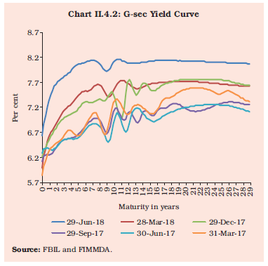

II.4.13 Yields continued to trade on an elevated note through Q3 in an environment of rising inflation, firming crude oil prices, announcement effects surrounding the intention of GoI to engage in additional borrowing of ₹500 billion and concerns over weak revenue collection through the GST. Pessimism stemming from the impact of the imminent issuance of public sector bank (PSB) recapitalisation bonds and consequent over supply of paper in the market also weighed down bond prices. The upgrade of India’s sovereign rating by Moody’s Investors Service and the cancellation of scheduled OMO sale by the Reserve Bank in November 2017 calmed sentiments briefly. However, G-sec yields started hardening again during December 2017 due to the announcement of additional borrowing of ₹500 billion by the GoI, rising crude oil prices and higher inflation prints.

II.4.14 During Q4, the auction of a new ten-year benchmark security in January 2018 lifted the mood of the market, supported by the announcement by the GoI of pruning down its additional borrowing requirement for 2017-18 to ₹200 billion. However, spillovers from global bond sell-offs in February and March dispelled this interlude even as fiscal slippages for 2017-18 and 2018-19 indicated in the Union Budget brought back concerns about excessive issuances. However, intermittent softening in crude oil prices and softer February consumer price index (CPI) inflation reading helped to cap the hardening of yields. Additionally, the Reserve Bank’s announcement of issue of longer term variable rate repos for addressing the financial year-end liquidity demand improved the market sentiment. During March 2018, domestic yields started trading with a softer bias, aided by absence of fresh supply of papers during the month, the GoI’s announcement of lower market borrowing in H1 of 2018-19 and maturing of ₹ 1 trillion worth of MSS T-Bills, which allayed liquidity shortage related concerns.

II.4.15 During Q1 of 2018-19, the yields initially softened in April in response to the dispensation given to banks by the Reserve Bank for spreading out mark-to-market (MTM) losses over four quarters and reduction in inflation forecast for H1 by the MPC. Subsequently, the yields started hardening on higher crude oil price, higher CPI inflation print and increased SDL supply. Additionally, hardening of global bond yields, rising trade related tensions and policy rate hikes by the US Fed and the Reserve Bank also impacted the market sentiment. Intermittent softening in global crude oil prices and OMO purchases by the Reserve Bank helped in ameliorating the adverse impact, to an extent, thereby capping the hardening of yields. The domestic 10-year benchmark security yield closed at 7.90 per cent on June 29, 2018.

II.4.16 In terms of the Medium Term Framework, the investment limits for FPI in G-sec (including SDLs) was increased in a phased manner from ₹2,580 billion as on April 3, 2017 to ₹3,279 billion as on April 6, 2018, a year-on-year (y-o-y) increase of 27 per cent. FPI utilisation of the total available limit (inclusive of investments in SDL), which stood at 68.4 per cent on April 3, 2017, increased to 79.3 per cent as on March 28, 2018 before declining to 65.2 per cent at end-June 2018. An outflow of FPI investments to the extent of ₹225 billion was witnessed in Q1 of 2018-19 mainly due to expectations of faster than anticipated pace of normalisation of monetary policy by the US Fed and weakening of the Indian rupee. The situation has been further exacerbated by rising crude oil prices and trade related tension between the US and China. Several emerging market economies (EMEs) have witnessed debt outflows on account of FPIs offloading their investments with India being no exception.

3. Corporate Debt Market

II.4.17 The corporate bond market has been boosted by a number of measures taken to develop the market in recent years. Net outstanding corporate bonds increased by 14 per cent y-o-y to ₹27.4 trillion by end-March 2018, about 16.3 per cent of GDP. The average daily turnover in the corporate bond market also increased sharply to ₹74.6 billion during 2017-18 from ₹61.0 billion a year ago. The Securities and Exchange Board of India’s (SEBI’s) new framework introduced in June 2017 for consolidation and re-issuance of debt securities by minimising the number of International Securities Identification Numbers (ISINs) to issuers improved market liquidity. Furthermore, proposals contained in the Union Budget 2018-19, such as, mandating large corporates to use the bond market to finance one-fourth of their funding needs, lowering the regulatory investment grade to ‘A’ from ‘AA’, and the introduction of uniform stamp duty for issuance of bonds across the country, have paved the way for further development of the corporate bond market.

II.4.18 In line with G-sec yields, corporate bond yields softened during most part of H1 of 2017-18, supported by easing inflation, normal progress of the monsoon and the 25 bps cut in the policy repo rate by the Reserve Bank in August. However, this reversed in H2 of 2017-18 with corporate bond yields hardening persistently in tandem with the increase in G-sec yields and episodes of hardening of bond yields witnessed globally. Overall, the 5-year AAA rated corporate bond yield increased by 39 bps to 7.96 per cent during 2017-18. However, the spread over G-sec yields narrowed significantly during the year by 57 bps and 31 bps for 5-year and 10-year AAA rated corporate bonds, respectively, especially in H2, reflecting improvement in credit quality on higher corporate earnings, a stronger economic outlook and expectations of faster resolution of corporate insolvency (Chart II.4.3).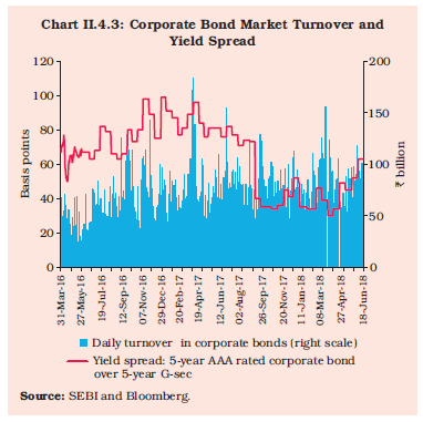

II.4.19 Primary corporate bond issuances declined by 9.8 per cent to ₹6,043 billion during 2017-18 from the peak level of ₹6,700 billion in 2016-17, which had surpassed the total bank credit extended during the year. The surge in bond yields in H2 tightened financial conditions, resulting in corporates shifting to bank credit for meeting their funding requirements. Public corporate debt issuances at ₹51.9 billion during 2017-18 were the lowest in the past eight years, as 99.1 per cent of the entire resource mobilisation from the corporate bond market was effected through the private placement route. FPI presence in corporate bond market increased to ₹2.2 trillion as at end-March 2018 from ₹1.9 trillion at end-March 2017. As a result, utilisation of the approved limit rose to 91.9 per cent from 76.0 per cent at end-March 2017.

II.4.20 Hardening of G-sec yields and increase in credit default risk, as reflected in higher credit default swap (CDS) spread, resulted in yield on 5-year AAA rated corporate bond hardening significantly by 81 bps to 8.78 per cent during Q1 of 2018-19. The yield spread of 5-year AAA rated corporate bond over 5-year G-sec widened by 24 bps. Consequently, primary issuances in corporate bond market declined by 33.6 per cent to ₹1,161 billion in Q1 of 2018-19 as compared with the corresponding period of the preceding year. The average daily turnover in the corporate bond market has increased to ₹75.0 billion in Q1 of 2018-19 as compared with ₹72.4 billion in Q1 of 2017-18.

4. Equity Market

II.4.21 The equity market was buoyed by strong rallies during 2017-18, with the benchmark indices scaling new peaks, tempered by intermittent corrections. The BSE Sensex and Nifty 50 increased by 11.3 per cent and 10.2 per cent, respectively, on the back of a combination of positive factors such as improved domestic macro-economic fundamentals and rallies in global markets (Chart II.4.4). The buoyancy in the domestic equity market was largely sustained by purchases by domestic mutual funds, though FPIs also lent support in the net.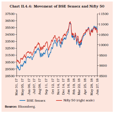

II.4.22 Commencing the year on a positive note, equity markets registered gains during April-May 2017 on the anticipation of a normal monsoon, the amendment to the Banking Regulation Act to tackle stressed assets, a sharp fall in retail inflation and finalisation of the GST rates. However, the market turned volatile soon after, with the equity indices registering declines during June 2017 following the announcement of farm loan waivers by some state governments, the Reserve Bank stipulating higher provisioning for bank loans submitted under the insolvency process and the second interest rate hike in 2017 by the US Fed.

II.4.23 Buoyancy returned to the equity market in July 2017 after the introduction of GST and release of the minutes of the US Fed’s June meeting, which reflected a lack of consensus on the future pace of rate hikes. However, market sentiment was adversely impacted in August 2017 by lower than expected corporate earnings for Q1 of 2017-18. Bearish sentiment continued to prevail in September 2017 on concerns relating to fiscal slippage, net selling by FPIs, geo-political tensions in the Korean peninsula and the US Fed’s announcement of balance sheet reduction/tapering off of reinvestment of maturing securities from October 2017. However, the market bounced back sharply in October on announcement of measures to recapitalise PSBs, improving macroeconomic conditions, upbeat corporate earnings results for Q2 of 2017-18 and revival of FPI. This was followed by a correction in November, notwithstanding a sharp jump in India’s ranking in the World Bank’s ease of doing business and the ratings upgrade by Moody’s, but the rally resumed in December triggered by Gujarat assembly election results and positive global cues.

II.4.24 The upswing gathered strength in January 2018 with the Sensex crossing the 36,000 mark and touching a historic high – 36,283 on January 29 - on positive cues from global markets, the upbeat macroeconomic outlook, encouraging corporate earnings results in Q3 of 2017-18 and optimism ahead of the Union Budget. This buoyancy was, however, associated with heightened volatility, particularly from the second half of January 2018 (Box II.4.1). The stock market witnessed a sharp correction in February 2018 on global sell-offs triggered by stronger than expected jobs and inflation data for the US and surge in the US bond yields. Adverse reactions to Union Budget proposals and concerns regarding GoI breaching the fiscal deficit target for 2017-18 further exacerbated the situation, with the Sensex declining by around 5 per cent to close the month at 34,184. Sentiments in the equity market continued to remain subdued in March with the BSE Sensex declining by 3.6 per cent to close the year at 32,969, triggered mainly by worries of trade conflicts between the US and China following the US announcement of tariffs on its steel and aluminium imports and proposals to impose import tariffs on Chinese goods, coupled with mixed domestic macroeconomic data releases.

Box II.4.1 Equity Indices and Implied Volatility Financial asset price volatility captures the frequency and magnitude of financial price movements - both up and down - over a certain period of time. Episodes of intense market volatility create uncertainty, as firms postpone their investment decisions and consumers halt their purchases. Volatility in asset prices can be measured as historical/ realised, based on historical returns, or implied/expected, based on markets expectations of future price movements. A simple measure of realised financial asset return volatility is its variance over time but this does not capture volatility clustering for which generalized autoregressive conditional heteroskedasticity (GARCH) is used. GARCH is a standard method for measuring asset return volatility, which captures volatility clustering, i.e., periods of turbulence followed by periods of calm, by measuring conditional variance, which takes into account the past history of returns. With increasing volumes of options and futures trading, implied volatility indices have gained significance because of their advantage of being forward looking, i.e., based on market expectations. Movements in implied volatility provide an almost instantaneous measure of the level of uncertainty in the market. The Volatility Index (VIX), also called the fear index, was introduced by the Chicago Board Options Exchange (CBOE) in 1993. The VIX, which is based on options in the S&P 500 index, measures market expectations of future volatility of the broad US stock market over the next 30 days. In India, the National Stock Exchange (NSE) introduced India VIX in March 2009 using the computation methodology of the CBOE, with suitable amendments. India VIX captures short-term expected volatility of Nifty 50, computed on the basis of order books of the underlying out-of-the-money Nifty options. The best bid-ask quotes of near and next-month Nifty options contracts, which are traded on the futures and options segment of the NSE, are used for computation of the India VIX which reflects not only investors’ expectations of volatility but also the premium they require to bear volatility risk. The formula used in the calculation is as follows: 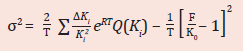where: σ is India VIX/100, which implies India VIX= σ x 100; T is time to expiration; Ki is strike price of ith out-of-the-money option; a call if Ki > F and a put if Ki < F; ΔKi is interval between strike prices - half the distance between the strike on either side of Ki; R is risk-free interest rate to expiration; Q(Ki) is the midpoint of the bid-ask quote for each option contract with strike Ki ; F is the forward index taken as the latest available price of Nifty future contract of corresponding expiry and K0 is first strike below the forward index level, F. There exists a significant negative and asymmetric relationship between stock returns and implied volatility (Schwert, 1989). Negative return shocks have a larger impact on implied volatility than positive return shocks. The negative correlation between implied volatility and the stock return is based on two fundamental hypotheses: the volatility feedback effect and the leverage effect. The volatility feedback hypothesis (French et al., 1987) posits that a sharp fall in the stock price leads to an increase in the risk premium due to anticipated increase in volatility, leading to an increase in VIX. On the other hand, the leverage effect (Black, 1976) indicates that a decline in a company’s stock price makes it more leveraged since the relative value of its debt rises and this induces a perception of the stock being riskier and, hence, more volatile. In India, the long term inverse relationship between India VIX and Nifty 50 turned positive during the second half of January 2018 when both the indices increased in tandem (correlation coefficient = 0.88 for January 2018). This points to market’s apprehension that the index had increased excessively and a correction was imminent. Global markets also witnessed a similar phenomenon as the S&P 500 and VIX moved together during that period (correlation coefficient = 0.70). However, sharp corrections in the equity market in the first week of February 2018 and heightened volatility led to the restoration of the long-term inverse relationship between the two. The India VIX increased sharply by 25 per cent to 20.02 on February 6, 2018, its highest level since November 2016. This was mainly on account of spillover of global volatility triggered by the rising US bond yields. The volatility in the global market was exacerbated by collapse of several complex volatility-linked funds and algorithmic trading strategies tied to market volatility. Market participants indicated that technical factors in options products and short-volatility strategies amplified market moves. The put-call ratio, which is a ratio of number of traded put options to number of traded call options, and is an indicator of investor sentiment, broadly remained stable and stayed below one in India during the period Jan 2017-Mar 2018. 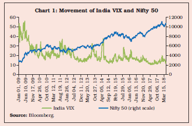Table 1: Correlation Coefficient between Stock Market Index And VIX Stock market/ VIX Jan 2009 - apr 2018 Jan-18 Feb-18 Nifty 50 and India VIX -0.72 0.88 -0.31 S&P 500 & VIX -0.68 0.70 -0.86 Source: RBI staff estimates. An estimation of the relationship between Nifty 50 and India VIX over a longer period, i.e., January 2009 to April 2018, indicated a significantly negative correlation between the two [(-) 0.72] (Table 1 and Chart 1). The Nifty 50 index and India VIX moved in the same direction, both positive and negative, 32 per cent of the time during the period of analysis. To assess the asymmetric nature of relationship between changes in the Nifty 50 index and India VIX for the period January 2010-January 2018, Newey-West estimator based regression has been used to overcome heteroscedasticity and autocorrelation in the error terms. Dummy variables have been used for positive and negative returns (Giot, 2005). The regression equation is given below: The results are presented in Table 2 below: Table 2: Estimated Coefficients of the Regression β+0 β-0 β+1 β-1 R2 -0.003 -0.011 -2.27 -4.36 0.36 (0.17) (0.00) (0.00) (0.00)   Note: p - values are given in parenthesis. Source: RBI staff estimates. It is evident that a significant negative and asymmetric relationship exists between India VIX and Nifty 50 returns, as the coefficient β-1 is larger in absolute value than β+1, which implies that the negative return shocks have a larger impact on implied volatility than positive return shocks. Additionally, realised volatility of stock returns, represented by conditional variance estimated through GARCH, and implied volatility, represented by VIX in the case of both Nifty 50 and S&P 500, generally moved in tandem. The realised volatility generally remained lower than expected volatility. However, during periods of extreme volatility, realised volatility estimated through GARCH rose above the implied volatility (Chart 2). Thus, short-term expected volatility, represented by VIX, is able to capture the realised volatility, as reflected by the co-movement of the two, but there is also value to employing realised volatility to understand price fluctuations. References: 1. Black, F. (1976). ‘‘Studies of Stock Price Volatility Changes.’’ Proceedings of the 1976 Meetings of the American Statistical Association, Business and Economic Statistics. 2. French K.R., G.W. Schwert and R.F. Stambaugh (1987), “Expected stock returns and volatility”, Journal of Financial Economics, 19(1), 3–29. 3. Giot, P. (2005), “Relationships between Implied Volatility Indexes and Stock Index Returns”, Journal of Portfolio Management, 26, 12-17. 4. Schwert G.W. (1989), “Why does stock market volatility change over time?”, Journal of Financial Economics, 44(5), 1115–1153.

II.4.25 Buoyancy returned to the equity market in 2018-19 with the BSE Sensex and Nifty 50 increasing by 7.4 per cent and 5.9 per cent, respectively, during Q1 of 2018-19 mainly on account of GoI’s announcement of a lower-than-expected market borrowing programme for the first half of 2018-19, better than expected corporate earnings results for Q4 of 2017-18, higher GDP growth for Q4 of 2017-18, positive economic activity data and forecast of normal monsoon in 2018 by the India Meteorological Department (IMD). After increasing sharply during April 2018, the markets witnessed intermittent corrections during May-June 2018, on concerns relating to prospects of trade related tensions between the US and China, political uncertainty in Karnataka, surge in crude oil prices and interest rate hike by the US Fed.

II.4.26 Sustained net investments by institutional investors, particularly mutual funds, during the year, provided upside momentum to equity markets, even as foreign portfolio flows turned volatile (Chart II.4.5). Net investment by mutual funds in equities during the year at ₹1,418 billion was much higher than ₹223 billion by foreign portfolio investors. During Q1 of 2018-19, mutual funds made net purchase of ₹335 billion, while foreign portfolio investors registered net sales of ₹204 billion.

Primary Market Resource Mobilisation

II.4.27 The primary segment of the equity market continued to be an important source of resource mobilisation. New equity issues, including qualified institutional placement (QIP), increased significantly during 2017-18, spurred by the buoyancy in the secondary market. Initial Public Offers (IPOs) and rights issues increased more than three times to ₹1,052 billion from ₹325 billion in the previous year. Companies mobilised a total of ₹838 billion through 200 IPO issues, out of which 155 issues amounting to ₹23 billion were listed on the small and medium enterprises (SMEs) platforms of the BSE and the NSE. During September-November 2017, a sharp rise in IPO activity was led by insurance companies, which accounted for 52 per cent of the total resources raised through IPOs in 2017-18. Resource mobilisation through QIP also jumped manifold from ₹85 billion in 2016-17 to ₹673 billion in 2017-18 mainly driven by increased capital requirements for banks under Basel III norms.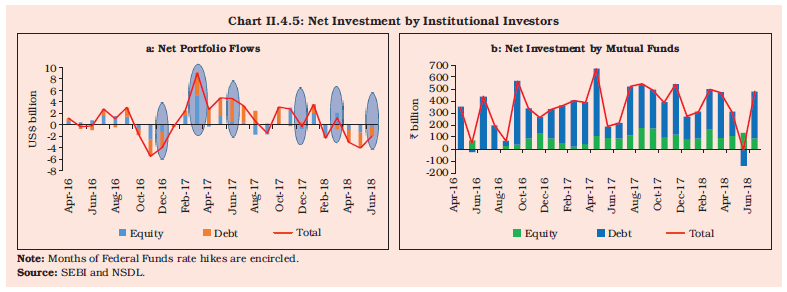

II.4.28 The net resource mobilisation by mutual funds declined by 20.8 per cent to ₹2,718 billion in 2017-18. However, resource mobilisation through equity and equity-oriented schemes more than doubled from ₹704 billion in 2016-17 to ₹1,711 billion in 2017-18, mainly driven by increased participation from retail investors and high net worth individuals (HNIs) who preferred equities over debt to earn higher returns. Accordingly, assets under management (AUM) of equity oriented schemes of mutual funds increased by 37.9 per cent from ₹5.4 trillion at end-March 2017 to ₹7.5 trillion at end-March 2018.

II.4.29 Primary market resource mobilisation through public issues of equity declined by 31.5 per cent (y-o-y) during Q1 of 2018-19. QIP issues also declined significantly by 85.2 per cent during Q1 of 2018-19. The net resources mobilisation by mutual funds increased by 43.4 per cent during Q1 of 2018-19.

5. Foreign Exchange Market

II.4.30 In the foreign exchange market, turnover picked up amidst broadly stable conditions during 2017-18. The INR traded with an appreciating bias against the US dollar in H1 of 2017-18 before depreciating in September 2017. Strong portfolio purchases, especially in the debt market, provided upside to the INR. Inflows on account of Masala Bonds and foreign direct investment supported the INR in July and August. However, geo-political tensions and the US Fed’s announcement of commencement of normalisation of monetary policy pulled the INR down in September 2017.

II.4.31 In the early part of H2, the INR traded with an appreciating bias during October before weakening against the US dollar in the first two weeks of November, as political turmoil in the Middle East and the knock-on impact of international crude oil prices clouded sentiments (Chart II.4.6). FPI purchases in the Indian debt market and a weakening US dollar supported the market in December and early January. However, re-emergence of concerns around the repercussions of elevated energy prices on India’s current account deficit (CAD), uncertainty around recalibration of the speed of monetary policy tightening by the US Fed upon arrival of strong wages and employment data, and the introduction of the long term capital gains (LTCG) tax domestically exerted downward pressure on the INR in the second half of January and in February. These pressures were accentuated by the strengthening of the US dollar, sales by FPIs in the equity and debt markets in India, and upward revision of fiscal deficit targets by the GoI. Overall, the rupee depreciated marginally by 0.3 per cent at end-March 2018 from its level a year ago although it appreciated in 2017-18 relative to the previous year on an average basis.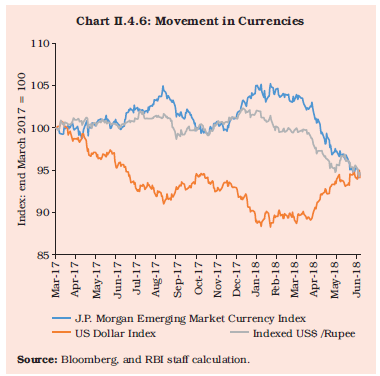

II.4.32 Rupee remained generally weak during Q1 of 2018-19 tracking broad-based gains in US dollar, sustained rise in crude oil prices and persistent FPI outflows from the Indian debt segment. The rupee staged intermittent recovery, especially towards end-May, due to softening of crude oil prices on prospects of higher production and better than expected Q4 growth but the gains could not be sustained in June due to significant hardening of crude oil prices, increase in CAD for Q4 of 2017-18, rate hike by the US Fed and intensification of trade related tensions between the US and China.

II.4.33 Forward premia recovered from post-demonetisation lows during 2017-18, although they continued to rule easy, reflecting the stability in the spot market. Turnover in both merchant and the inter-bank segments of the spot market and swap segment picked up, whereas the forward segment exhibited a minor reduction in activity.

II.4.34 Going forward, global risk factors like geo-political developments in the Middle-East leading to sharp increase in crude oil prices, faster than anticipated pace of rate hike by the US Fed and increase in protectionism leading to prospects of trade related tensions could induce volatility in the domestic financial markets. However, sound domestic macro-economic fundamentals would provide a strong bulwark against any externally induced volatility spillovers.

II.5 Government Finances¹⁶

II.5.1 In 2017-18, public finances were marked by deviations from budgetary deficit targets at both central and sub-national levels, essentially from the revenue account. For the central government, the pressure points turned out to be indirect tax collections, non-tax revenue and revenue expenditure. The late implementation of GST (in July 2017) and the teething problems that followed in its wake did not deter indirect tax collections from exceeding the preceding year’s level but the rising buoyancy of the preceding two years was interrupted and the indirect tax to GDP ratio dipped. The shortfall in non-tax revenue relative to budget estimates (BE) needs to be viewed in the context of deferment of spectrum auctions, the acute stress in balance sheets of banks and corporates that eroded profitability, and the costs of demonetisation impinging on the balance sheet of the Reserve Bank. With revenue expenditure programmed to expand due to upward revisions in salaries, pensions and allowances of central government employees and defence personnel, capital expenditure had to be pruned from the budgeted amount. In the event, the provisional accounts (PA) for 2017-18 show that the centre’s gross fiscal deficit (GFD) at 3.5 per cent of GDP was higher than the budgeted 3.2 per cent of GDP.

II.5.2 The consolidated GFD of states in 2017-18 as per revised estimates (RE) at 3.1 per cent of GDP exceeded the budgeted target (2.7 per cent of GDP). The main underlying factors were shortfall in own tax revenues and higher revenue expenditure on account of pay commission award and farm loan waivers.

II.5.3 For 2018-19, the centre’s GFD is budgeted at 3.3 per cent of GDP, a reduction of 0.2 percentage points over the 2017-18 level. The fiscal deficit target of 3.0 per cent has been deferred to 2020-21. In case of states, the budget estimates of the consolidated fiscal deficit at 2.6 per cent need to be seen in light of the recent historical record and the gaps in the institutional architecture, the latter attracting new scrutiny in the context of the farm loan waivers and the implementation of the pay commission recommendations. Notwithstanding some moderation in the post crisis period, the general government GFD has remained above 6.5 per cent of GDP since 2012-13. It is estimated to be around 6.6 per cent in 2017-18 (RE) and is budgeted at 5.9 per cent in 2018-19.

1. Central Government Finances in 2017-18

II.5.4 The fiscal strategy for 2017-18 was centered on the rural economy, infrastructure and poverty alleviation while persevering with structural reforms, including in-budgetary processes such as the advancement of the budget presentation to February 1, merger of the railway budget with the Union Budget, and the abolition of the plan and non-plan classification of expenditure. In terms of actual outcomes, centre’s tax revenues net of devolution to states exceeded the budgeted amount by 1.3 per cent, sustaining the upturn in the tax/GDP ratio that commenced in 2016-17. Underlying this improvement, gross direct tax revenues were buoyed by higher collections under income and corporate taxes, with growth rates of 12.0 per cent and 17.8 per cent, respectively. With corporate tax buoyancy being higher than in 2016-17, corporate tax collections also exceeded the budget estimates of 2017-18. Unlike the direct tax to GDP ratio, the indirect tax to GDP ratio declined marginally in 2017-18, although collections exceeded the previous year’s receipts by 5.9 per cent.

II.5.5 Non-tax revenues recorded a shortfall of 33.3 per cent from budgetary targets, mainly on account of lower receipts from interest, dividends and profits. The Reserve Bank transferred an overall surplus of ₹306.6 billion to the government in 2017 as against ₹658.8 billion in 2016, a decline of 53.5 per cent. In 2017-18, aggregate dividend receipts were lower by 35.8 per cent than the BE and by 25.7 per cent over their 2016-17 level. Notably, net receipts from communication services fell short of BE mainly because of deferment of spectrum auctions. On the other hand, proceeds of ₹1 trillion from disinvestment on the back of strategic sales were the highest in any financial year so far and exceeded the BE by 38.2 per cent. Reflecting these constituent movements, total non-debt capital receipts registered a growth of 77.2 per cent vis-à-vis 3.8 per cent in the previous year.

II.5.6 Revenue expenditure exceeded the budget target by 2.3 per cent on account of higher pension and interest payments, absorbing the entire increase in non-debt capital receipts. Consequently, capital expenditure had to be pruned below the BE by 14.9 per cent in contrast to the healthy improvement in 2016-17 when capital expenditure was protected and the burden of adjustment fell on revenue expenditure.

II.5.7 Reflecting these developments, the budgeted target for GFD-GDP ratio at 3.2 per cent was breached by 0.3 percentage points in 2017-18. The revenue deficit (RD)-GDP ratio at 2.6 per cent shows a deviation of 0.7 percentage points from the BE, more than double the deviation in the GFD-GDP ratio (Table II.5.1).

2. Central Government Finances in 2018-19

II.5.8 The Union Budget for 2018-19 renewed the emphasis on reviving rural demand by focusing on the rural economy and agriculture. In contrast to 2017-18, the fiscal strategy expanded its ambit to the social sector (education, health and social welfare) and maintained its thrust on infrastructure and the financial sector, the latter through the announcement of important measures like bank recapitalisation and introduction of the standing deposit facility. Although the fiscal cost of bank recapitalisation bonds is yet uncertain, the measure could lend tailwinds to the recent recovery in bank credit and, in turn, overall growth, compensating for any additional interest burden on the government in the interim. The step-up in allocations is sought to be financed by augmenting tax collections and by sustaining the disinvestment drive.

II.5.9 The central government accepted the medium-term fiscal targets recommended by the Fiscal Responsibility and Budget Management (FRBM) Review Committee (Chairman: Shri N. K. Singh) but with a delayed timetable. The FRBM Review Committee had recommended a medium term GFD-GDP target of 2.5 per cent for the centre by 2022-23. Furthermore, the Committee recommended that the combined GFD should be reduced to 5 per cent of GDP, equally divided between the centre and states. As against this, the GFD target of 3.0 per cent for the centre has now been shifted from 2018-19 to 2020-21, while the central government debt will be brought down to 40 per cent of GDP by 2024-25, two years later than recommended. The government also agreed to explicit escape and buoyancy clauses. On the ground or grounds of national security, act of war, national calamity, collapse of agriculture severely affecting farm output and incomes, structural reforms in the economy with unanticipated fiscal implications, decline in real output growth of a quarter by at least 3 per cent points^* below its average of the previous four quarters, the annual fiscal deficit target may be exceeded/deferred. Any deviation from the fiscal deficit target, however, shall not exceed one-half per cent of GDP in a year. The central government shall, in case of increase in real output growth of a quarter by at least 3 per cent points^* above its average of the previous four quarters, reduce the fiscal deficit by at least one-quarter per cent of GDP in a year. Under situations where the fiscal deficit is allowed to vary from the prescribed target despite increase in GDP growth, the government shall lay, before both the Houses of Parliament, a statement explaining the reasons thereof and the path of return to annual prescribed targets.

II.5.10 The GFD for 2018-19, is budgeted at 3.3 per cent of GDP, vis-à-vis the 2017-18 outcome of 3.5 per cent. Given the expenditure priorities of the fiscal strategy, the realisation of the budgeted GFD hinges on the centre’s revenue effort – 18.3 per cent growth in gross tax revenues; 22.3 per cent in indirect taxes with GST collections increasing by 70.5 per cent. Underpinning the projections of gross tax revenue is an implicit tax buoyancy of 1.45 in 2018-19 (BE) although higher than the realised buoyancy of 1.19 in 2017-18. The average buoyancy in personal income tax was higher at 2.5 and 1.2 for 2016-17 and 2017-18, respectively, as against 1.0 during the seven years from 2009-10 to 2015-16. This is attributable to the ongoing tax base broadening and enforcement measures. Receipts from non-tax revenues are budgeted to increase in 2018-19 by 27.3 per cent, with major contributions from interest receipts, followed by non-tax receipts of Union Territories. Encouraged by the disinvestment outcomes in 2017-18, the target for disinvestment has been projected at ₹800 billion in 2018-19 (BE).

II.5.11 Total expenditure is budgeted to grow by 14.0 per cent in 2018-19 (8.5 per cent in 2017-18). Capital outlay (i.e., capital expenditure excluding loans and advances) is projected to grow by 13.9 per cent (1.3 per cent decline in 2017-18). Capital expenditure is budgeted to grow at 13.9 per cent, with emphasis on transport and social welfare (Chart II.5.1). Expenditure on major subsidies, viz., food, fuel and fertiliser is budgeted to rise by 38.3 per cent to 1.4 per cent of GDP from 1.1 per cent of GDP in 2017-18.

II.5.12 As per the latest information available, RD and GFD, both in absolute terms as well as per cent of BE were lower during April-June 2018 as compared to the corresponding period of the previous year, since the growth in revenue receipts surpassed that in total expenditure. Non-tax revenue also surged during the quarter. The growth in total expenditure was mainly driven by capital expenditure.

3. State Finances in 2017-18

II.5.13 Fiscal position of 29 state governments at a consolidated level points toward deterioration in key deficit indicators in 2017-18 (RE) as against the BE. The erosion occurred despite no issuances of bonds under the UDAY scheme, which had resulted in higher deficits in the preceding two years. Revised estimates for 2017-18 indicate a deviation of 0.40 percentage points of GDP in the consolidated states’ revenue deficit and 0.35 percentage points in the GFD from the budget estimates. The deviation has occurred on account of both overshooting of revenue expenditure by 13 basis points (bps) due to farm loan waivers and other factors, which include pay revisions and shortfall of revenue receipts by 27 bps, mainly reflecting a decline in states’ own taxes by 0.33 per cent of GDP. This shortfall was partly offset by transfers from the centre, which exceeded budget projections by 0.09 per cent of GDP. Fiscal consolidation and any deviation therefrom may have implications for macroeconomic stability and inflation, in particular (Box II.5.1).

4. State Finances in 2018-19

II.5.14 For 2018-19, states have budgeted for a consolidated GFD of 2.6 per cent of GDP. The correction mainly emanates from the revenue account, which is projected to post a surplus of 0.2 per cent of GDP [deficit of 0.4 per cent in 2017-18 (RE)] (Chart II.5.2). Revenue receipts are expected to go up on account of central transfers and states’ own taxes comprising states’ GST and other commodity taxes. Notwithstanding the consolidation in GFD-GDP ratio budgeted for 2018-19, eleven states are projecting a fiscal deficit above the 3 per cent threshold. With fiscal marksmanship of states being weak (RBI, 2018)¹⁷, any shortfall in the revenue account will imply that capital expenditure may have to bear the brunt of the fiscal correction as it has done over the past two years. Spending pressures pose further risks, including from farm loan waivers, and ongoing implementation of the pay commission recommendations.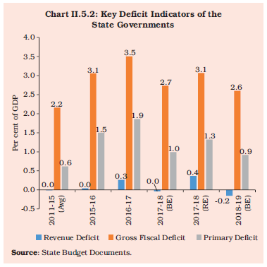

Box II.5.1 Relationship between Fiscal Policy and Inflation: Results from Quarterly Projection Model India has adopted the flexible inflation targeting framework with consumer price inflation as the nominal anchor for monetary policy. Policy models like Quarterly Projection Model (QPM) (Benes et al., 2016) under the Forecasting and Policy Analysis System (FPAS) play a critical role in ensuring consistent forward looking assessment and evaluation of the risks to baseline path over the medium term. In recent past, there have been growing concerns on the implications of the fiscal deficit at central and state levels for durable disinflation and achievement of the target. Empirical results for the recent period suggest a positive and statistically significant long-run relationship, leading from fiscal deficits to inflation in India, which is non-linear in nature, i.e., the impact of fiscal deficit on inflation will be higher at higher levels of the fiscal deficit and inflation (Mitra et al., 2017). This box presents the results of the introduction of a fiscal block in the QPM to validate the role of fiscal policies on aggregate demand and overall inflation (Raj et al., 2018). QPM is a forward-looking open-economy calibrated gap model based on the New-Keynesian framework and incorporates a number of India-specific characteristics of inflation process and monetary policy transmission. In QPM, fiscal stance influences inflation outcomes through its impact on aggregate demand and exchange rate. The overall fiscal deficit, based on the IMF and OECD approach, is decomposed into structural and cyclical deficits to arrive at the structural or the underlying fiscal position when cyclical or automatic movements are removed. Cyclical deficit captures the movements in government revenue and expenditure in line with the rise and fall of economic activity and hence cyclical deficit is modelled as a function of output gap. The cyclically adjusted fiscal deficit or the structural deficit then represents the underlying or structural components of fiscal balance that do not self-correct with change in economic cycle. Government consumption shock is seen to induce private consumption and real demand. The unanticipated changes in structural deficit and deviations from debt target are formulated to have an impact on domestic economic cycles. Further, the deviation from the long-term debt target will affect the country risk premium and hence the exchange rate through the uncovered interest parity (UIP) condition. The conceptual framework for augmenting fiscal block in the QPM is presented in Chart 1. 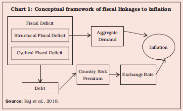Augmenting the fiscal block to the QPM and analysing the historical decomposition of the output gap (Chart 2) in the post-GFC (i.e., global financial crisis) period clearly bring out the role of large fiscal deficit when the FRBM Rule based fiscal consolidation was set on a ‘pause’. Subsequently, the re-implementation of fiscal rules from 2012 has helped to temper the demand side pressures and in turn inflation. Further, the simulations from QPM after taking into account the non-linear impact of fiscal deficit on inflation, presented in Chart 3, suggests that at a level of four per cent inflation and six per cent combined fiscal deficit to GDP ratio, one percentage point shock to structural fiscal deficit to GDP ratio, would push the inflation up by around 40 bps over three-year period. However, its impact gets magnified, if the inflation and combined fiscal deficit are at higher levels. In this context, the recent monetary policy statements have highlighted the importance of the adherence to budgetary targets by the centre and the states in achieving the medium-term target for headline inflation of 4 per cent on a durable basis. 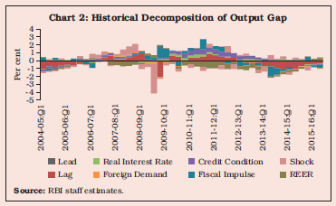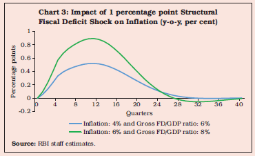References: 1. Benes, M. J., K. Clinton, A. T. George, P. Gupta, J. John, O. Kamenik, D. Laxton, P. Mitra, G. V. Nadhanael, R. Portillo, H. Wang and F. Zhang (2016). “Quarterly Projection Model for India: Key Elements and Properties”. RBI Working Paper, November. 2. Mitra, P., I. Bhattacharyya, J. John, I. Manna and A. T. George (2017), “Farm Loan Waivers, Fiscal Deficit and Inflation”, Mint Street Memo No.5, Reserve Bank of India. 3. Raj, Janak, P. Mitra, A. T. George and J. John (2018), “Monetary Fiscal Interaction in an Inflation Targeting Framework - Recent Evidence from India”, Reserve Bank of India, mimeo.

5. General Government Finances

II.5.15 The general government GFD, which was in a consolidation phase from 2012-13 started deteriorating from 2015-16 to reach 7.0 per cent of GDP in 2016-17. While the centre sustained its consolidation process during the period, the states used up the fiscal space more than that vacated by the centre, keeping the combined GFD-GDP ratio at an elevated level. However, the general government GFD is budgeted to be 5.9 per cent of GDP in 2018-19 as against 6.6 per cent in the revised estimates for 2017-18.

II.5.16 Globally, general government balances across G-20 countries present a mixed picture (Table II.5.2). While countries such as Russia and Mexico strengthened fiscal consolidation in 2017, the situation deteriorated in Argentina, China and South Africa as also in the US and Japan. In Brazil and India, general government deficits continue to rule at elevated levels.

II.5.17 Outstanding liabilities of the general government are budgeted to decline to 68.3 per cent of GDP at end-March 2019 from 68.9 per cent at end-March 2018 (RE). As per the revised FRBM architecture, the aim is to attain a central government debt to GDP ratio of 40 per cent and a general government debt to GDP ratio of 60 per cent by 2024-25. The definition of central government debt has also been widened to include all outstanding liabilities, including those in the Public Accounts. Further, the external debt has to be valued at the current exchange rate henceforth. The amendment further states that the central government shall not give additional guarantees with respect to any loan on security of the Consolidated Fund of India in excess of one-half of one per cent of GDP in any financial year. Though the current debt levels are above the FRBM target, the debt servicing capacity of the general government has improved over the previous two years with the interest payments as per cent to revenue receipts exhibiting a decline (Chart II.5.3).

II.5.18 The central government reported an expansionary fiscal impulse for 2017-18, driven by underperformance in non-tax revenue, indirect taxes and revenue expenditure. It was also witnessed at the level of states in respect of the GFD, the revenue deficit and the primary deficit in 2017-18 (RE), along with a deterioration in their debt position. Going forward, centre and states may have to withstand revenue expenditure pressures due to farm loan waivers, pay commission recommendations for states, likely rise in fuel subsidies and a higher interest burden associated with rising market borrowings and elevated yields. However, the broadened tax base achieved through structural reforms coupled with enhanced GST compliance and increased tax efficiency via successful implementation of the E-way bill, could help both centre and states in meeting these pressures successfully and in getting back to the path of fiscal consolidation over the medium term. This will help assuage market sentiment, in turn contributing towards lower interest and debt burden for the general government.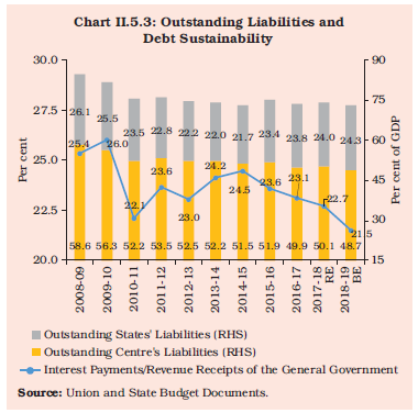

II.6 EXTERNAL SECTOR

II.6.1 Just as the international environment was improving with global trade outpacing global growth in 2017 and capital flows to EMEs rebounding after bouts of reversals during 2013-16, it has been unsettled by the intensification of protectionism and retaliatory strategies that threaten to rend asunder the institutional fabric of multilateral trade. These developments have adverse implications for advanced economies (AEs) and EMEs which have sought to harness international trade as a handmaiden of growth. Meanwhile, global financial markets have been re-pricing the normalisation of monetary policy by systemic central banks which, in turn, has resulted in sell offs in bond and equity markets, realignment of major currencies and considerable flux in capital flows.

II.6.2 Against this backdrop, India’s external sector exhibited resilience in the face of terms of trade losses due to the firming up of international crude prices and domestic supply constraints. As set out in the following two sub-sections, export performance improved in 2017-18 although domestic disruptions impeded a fuller response to the congenial conditions engendered by rising world trade. However, a sharp rise in imports partly due to price effects expanded the trade deficit to a five-year high. Notwithstanding the support from net invisible receipts profiled in sub-section 3, the current account deficit (CAD) widened during 2017-18 as set out in sub-section 4, but within sustainable norms and as sub-section 5 would portray, it was comfortably financed by net inflows of capital. While the level of India’s net international investment position (NIIP) deteriorated modestly with the increase in liabilities in the form of direct and portfolio investment as shown in sub-section 6, performance of other external vulnerability indicators was somewhat mixed over the year though there was a sizable accretion to international reserves.

1. Merchandise Exports

II.6.3 Global trade volume, which emerged towards the close of 2016 out of a 20-month sub-3 per cent y-o-y growth, gained strength and traction through 2017 peaking at 6.1 per cent in March 2017 (Chart II.6.1). For the year as a whole, world trade volume grew at 4.6 per cent, up from 1.5 per cent in the preceding year. A noteworthy feature of this rebound is that the income elasticity¹⁸ of world trade rose to 1.5 in 2017 for the first time after 5 years when it had fallen to 0.6. The recovery of world trade in 2017 was driven equally by AEs and EMEs.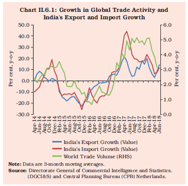

II.6.4 India’s merchandise export growth accelerated in 2017-18 and expanded by 10.0 per cent in US dollar terms, backed by volume growth of 5.3 per cent. A fuller response to the rising tide of world trade was, however, restrained by supply-side bottlenecks relating to liquidity, documentation and delays in refunds following the implementation of the GST (Box II.6.1). Effects of the fallout were most visible in exports of labour-intensive sectors such as gems and jewellery, readymade garments, carpets and handicrafts. By contrast, shipments of other major constituents, viz., engineering goods, chemicals and marine products, which account for a little more than 30 per cent of total merchandise exports (19.4 per cent, y-o-y growth), showed resilience and recorded growth rates ranging between 17.1 per cent and 29.2 per cent during 2017-18.

II.6.5 Since 2012-13, structural shifts in India’s export profile have been underway. First, the tradability of India’s output, measured by exports to GDP has been persistently declining, indicative of the declining export intensity of domestic growth. Second, in contrast to global developments, the income elasticity of India’s exports remained broadly stagnant in 2017-18. This suggests that the response of India’s export to global growth has been limited. Third, even as some peer economies have managed to build their market shares in key items of India’s export basket, India’s exports have faced erosion in terms of market presence. Consequently, the share of India’s exports in world exports has been constant at around 1.7 per cent of world exports in the last five years, possibly pointing to a protracted stagnation in competitiveness. In this context, Box II.6.2 examines various aspects of India’s export competitiveness in recent years. Overall export growth was largely pulled up by petroleum products which raised their share in total exports steadily to 12.3 per cent during the year. They were mainly supported by higher international prices as unit value realisations rose by 18.5 per cent, outstripping volume growth of 1.5 per cent during 2017-18.

Box II.6.1 Working Capital Constraints and Exports The implementation and refund delays under the new tax regime of Goods and Services Tax (GST) had reportedly led to working capital constraints for firms. In the absence of high frequency data, it is difficult to test this hypothesis using general economic activity indicators. In order to overcome this handicap, we looked at exports data as it is available at monthly frequency. We test whether the exports of sectors with high working capital requirements were hit more severely than those with low working capital requirements due to delay in GST refunds. If GST squeezed the funding due to delays in tax refunds, it should get reflected in export performance of sectors which are highly dependent on working capital. The GST implementation, in the beginning, was marred by infrastructure snags and implementation delays, which led to changing the date of filing July tax returns multiple times. Finally, firms were required to file their returns by September 30, under the latest revision. As per the implementation of the tax regime, exporters were supposed to get 90 per cent of the input tax refund within seven days of filing their returns. However, there were significant delays in receiving the input tax credit according to various reports, which could have adversely affected the working capital of firms. Analysis To test our central hypothesis, we look at the difference in exports growth between October and March 2017 for different sectors and trace if this is correlated with the sector-level working capital to sales ratios. More precisely, we check whether working capital to sales ratio for sector i helps explain the sectoral variation in the following double difference: The object in above equation is a difference in difference variable, where the first difference captures the change in exports between October and March 2017, i.e., impact of GST, while the second difference corrects for seasonality. If the GST implementation led to an export deterioration in October 2017 due to the mechanism espoused above, then we should expect a negative correlation between the above double difference and working capital to sales ratio. We indeed find that the relationship between the difference in export growth and working capital to sales ratio is negative and has a slope coefficient of −0.18 in October (Chart 1). It roughly implies that a 10 per cent increase in the working capital/sales ratio led to a 1.8 per cent decrease in the exports growth. The placebo test also shows that there is no significant relationship between exports growth difference between September and March, further establishing the relationship and favouring our central hypothesis (Chart 2). 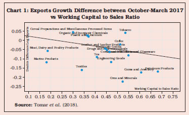Further, we use firm-level data from Prowess to test for the impact of GST on firm behaviour. If GST led to a negative liquidity shock, we should expect firms to increase their short-term borrowings, run down their cash and bank balances and reduce their capital expenditure. We run the following regression to test the validity of these hypotheses: where, Yit is the object of interest for firm i at time t and is one of the three outcome variables mentioned above. D(Sep ’17) is the dummy on Q3 2017, while D(Sep ’17) * (Working Capital/Sales) is the interaction of this dummy with working capital to sales ratio. The two coefficients of primary interest in equation (2) are β1 and β2. While β1 captures the general impact of Q3 2017 (D(Sep ’17)) on Yit , β2 captures the effect of Q3 2017 for firms with high working capital to sales ratio (at sector level) in Q3 2017. 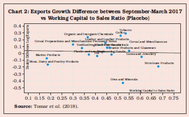Columns (1) and (2) in Table 1 show the impact of GST on the short-term borrowings of firms. The coefficient on Dummy (Sep ’17) is insignificant, showing no direct impact of GST, though β2 is significant in column 2 and shows a small but positive impact on short-term borrowings, i.e., firms in sector with high working capital requirements increased their short-term borrowing in September 2017. Here, it is important to mention that this regression is conditional on firms’ reporting short-term borrowings. So, the short-term borrowings increased for those firms that actually borrowed during this period as well as in the past. We also find that in Q3 2017, firms reduced their ‘cash and bank balance’ during this period as reflected in β1 coefficient in column 4. Lastly, the quarter dummies are negative though insignificant in the case of capital expenditure as shown in columns 5 and 6, which suggests that capital expenditure was not affected in this period. Given these results, we can conclude that firms primarily ran down their cash and bank balance during Q3 2017 in response to the GST shock to their short-term funding. Table 1: Empirical Results   Log (Short-Term Borrowing) Log (Cash and Bank Balance) Δ (Log Capital) (1) (2) (3) (4) (5) (6) β1 0.00421 -0.0386 -0.171*** -0.193*** -1.392 -1.388   (0.115) (0.124) (0.065) (0.0702) (0.739) (0.738) β2   0.00312**   0.00177   0.000239     (0.001)   (0.0006)   (0.0002) Firm FE Yes Yes Yes Yes Yes Yes Quarter FE Yes Yes Yes Yes Yes Yes Observations 16,436 14,171 23,332 20,213 19,292 17,934 Note: ***: Significant at 1 per cent **: Significant at 5 per cent Source: Tomar et al. (2018) In summary, we explore using the GST shock how short-term liquidity shock could impact firms in the export sector. We find that the sectors with high working capital/ sales ratio were hit the most due to the post-GST liquidity constraints. This is also corroborated by the various measures adopted by the government during November to address the concerns of the exporters. Finally, the rebound of exports in November 2017 [as reported in Tomar et al. (2018)] suggests these quick measures partly addressed the temporary credit constraints faced by the exporters during October 2017. Reference: 1. Tomar S., Mathur S and Ghosh S (2018), “Working Capital Constraints and Exports: Evidence from GST Rollout,” RBI Mint Street Memo, No. 10, February 12, 2018.

II.6.6 Among non-oil exports, engineering exports – mainly led by iron and steel, non-ferrous metals and automobiles – went up across the board to destinations in the European Union (EU), North America, Association of Southeast Asian Nations (ASEAN), Middle East and North Africa. Helped by the rise in international steel prices and subdued supply from China, India turned net exporter of steel for the second consecutive year and accounted for about 2 per cent of global exports in the category. Spurred by rising demand for frozen shrimp and a drastic reduction in rejection rates by EU countries brought about by quality enhancing measures in India, marine exports increased. Exports of chemicals benefitted from the market share foregone by China due to the implementation of stricter environmental laws by the Ministry of Ecology and Environment, China. Growth in exports of organic chemicals drove up chemical exports in 2017-18.

Box II.6.2 Measuring India’s External Competitiveness The multi-dimensional nature of export competitiveness renders its measurement and interpretation challenging. For instance, an increase in export growth relative to its past performance or relative to that of a competitor economy may arise not just because of improvement in competitiveness (price/cost competitiveness) but due to an advantageous mix of export markets and export products. Therefore, it may be desirable to use an array of indicators to assess a country’s export performance. Against this backdrop, this box identifies and quantifies measures of export competitiveness for India over time. The literature identifies a number of indicators to measure comparative advantage and cost competitiveness, i.e., the real effective exchange rate (REER); productivity; market shares; revealed comparative advantage (RCA); unit labour cost; Lafay Index (measure of RCA), Herfindahl-Hirschman Index (measures concentration) among others. A basic measure of export performance is to track a country’s share in world exports over time. On this metric, India’s share in world exports, which was just below 0.7 per cent in 2000 registered a 2.5 times improvement by 2017. This aggregate measure, however, does not reveal anything about the source of the improvement. The RCA metric analyses the relative trade performance of individual countries in particular commodities. The RCA is computed as the ratio of a commodity’s share in a country’s exports relative to the share of the commodity in total world exports (equation 1). The trade pattern of a commodity is assumed to reflect inter-country differences in relative costs as well as in non-price factors, “revealing” the comparative advantage of the trading countries. 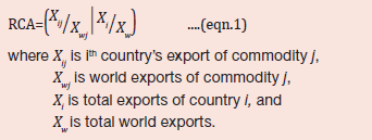A country is said to have comparative advantage in a particular sector if the RCA for that sector is greater than 1. An analysis of the RCA of the top five exports from India reveals a mixed trend. India’s RCA in pearls and precious stones has eroded considerably over 2006-2017 while there has been an increase in India’s RCA in textiles in 2017 (Chart 1). Nonetheless, India has been able to protect its relative advantage in the top five export sectors (mineral products, textiles, chemicals, base metals and pearls & precious stones). Although RCA is a widely accepted approach for assessing comparative advantage, it does not account for import trade flows, relative prices of commodities, supply and demand shocks and does not provide insights into the drivers of comparative advantage. 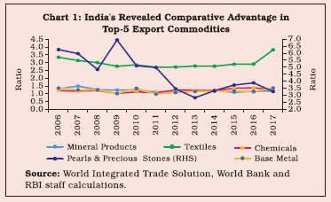As indicated earlier, change in a country’s market share could be driven by push factors (country-specific factors) or by shifts in the product mix or export market. Thus, the shifts in a country’s market share need to be decomposed into different segments to fully comprehend the underlying dynamics. In this context, export growth can be decomposed in a weighted analysis of variance (ANOVA) framework using disaggregated bilateral trade data (Gaulier et al., 2013). This method aids the assessment of export performance purged of product and geographic specialisation. The analysis reveals that between 2006 and 2016, India gained market share relative to many of its peers (Chart 2a). The contribution of push factors, shown in the chart as push-effect, was relatively strong in increasing India’s export market share during 2006-2010 though it has been negative or largely muted since 2010 (Chart 2b). Similarly, changes in product mix have generally had a negative contribution to export market share since 2010. Yet another measure of international competitiveness is the Real Effective Exchange Rate (REER). By construction, an increase in the REER index is associated with diminishing external (price/cost) competitiveness. The rise in the REER in the case of India is lower than for many peer economies (Chart 3). To summarise, measures of India’s external competitiveness present a mixed picture. While India has gained share in world exports over time, a decline in the RCA for a few products/sectors points towards diminishing comparative advantage even as India has been able to maintain its advantageous position in its top 5 export sectors. Similarly, a decomposition of changes in India’s export market shares reveals that while push factors were important in driving the change, it was also impacted by change in product and geographical mix. References: 1. Gaulier, G., G. Santoni., D. Taglioni., and S Zignago (2013), “In the Wake of the Global Crisis: Evidence from a New Quarterly Database of Export Competitiveness”, Policy Research Working Paper 6733, World Bank, Washington, December.

II.6.7 The top markets that absorbed half of the increase in India’s exports in 2017-18 included the USA, China, Hong Kong, Germany, Bangladesh and Vietnam. By contrast, exports to the United Arab Emirates, the third largest export destination, declined due to lower shipments of gems & jewellery and readymade garments, which shrank the bilateral trade surplus from a year ago (Chart II.6.2).

2. Merchandise Imports

II.6.8 Merchandise imports, which had spiralled down into a prolonged decline starting in December 2014, broke out of the contraction in October 2016 and rose sharply in 2017-18 peaking in April 2017 before losing some steam in ensuing months. A decomposition of these patterns through the upturn phase (October 2016 to March 2018) shows that the price impact dominated the volume effect during November 2016 – March 2017, coinciding with the sharp increase in international crude oil prices. The volume impact eclipsed the price impact during April 2017 to February 2018. The burgeoning import bill for petroleum crude and products largely reflected higher international crude oil prices as import volumes have broadly remained stable. International crude oil prices firmed up in response to production cuts imposed by the Organisation of Petroleum Exporting Countries (OPEC) and Russia, and supply shocks emanating from Venezuela which reduced global output by about 0.7 million barrels per day in 2017. These cuts are intended to remain in place till December 2018. Meanwhile, the rise in crude prices incentivised a ramping up of shale production in the US to record levels in 2017, augmenting global supply by 0.7 million barrels per day. Notwithstanding this development, the faster expansion of global demand by 1.7 million barrels per day has necessitated a drawdown of inventories by 0.5 million barrels per day in 2017 in the OECD countries, which drew a line under crude prices.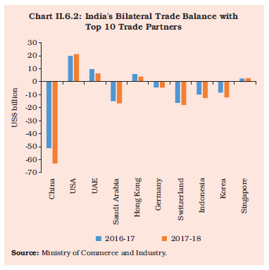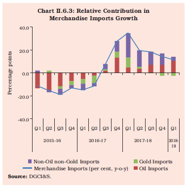

II.6.9 Gold imports at 955.2 tonnes were due to a rebound in domestic demand for the precious metal as jewellers replenished inventory amidst a turnaround in retail demand after demonetisation in the preceding year. Petroleum and gold together accounted for more than one-third of import growth in 2017-18 (Chart II.6.3).

II.6.10 Non-oil non-gold imports accounted for 65.1 per cent of total import growth on a weighted contribution basis as a part of domestic demand spilled into imports (Box II.6.3). Electronic goods, pearls and precious stones, coal, chemicals, machinery and iron and steel together contributed more than half of the growth in this segment (Chart II.6.4). Responding to unusually high imports of electronic goods, the government raised the basic customs duty for various electronic products like mobile phones including its parts and accessories, smart watches, and parts of televisions. Import duty was also increased on cut and polished gemstones, diamonds, and imitation jewellery. Domestic shortages of coal caused by lower production than the target set for Coal India Ltd. was met through higher imports. Imports of iron and steel remained high as restrictive measures undertaken in recent years eventually lost their efficacy, partly due to rupee’s appreciation. Korea, China and Japan were important sources of iron and steel imports. With import growth largely outpacing that of exports throughout the year, the merchandise trade deficit expanded to a five-year high. Since 2011-12, the trade deficit has averaged 7.3 per cent of GDP, making it pivotal in the overall balance of payments.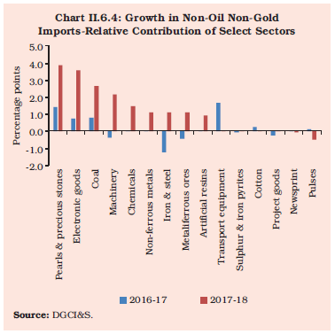

Box II.6.3 The Curious Case of Reverse Import Substitution: The Indian Experience During 2017-18, there was a surge in imports, especially in the category of non-oil non-gold items, which broke out of the traditional co-movement with export behaviour but coincided with a period of sluggish manufacturing activity. This has given rise to concerns that disruptions in the production/supply chain during post-demonetisation have forced domestic demand to spill over into imports in order to overcome domestic supply constraints. This phenomenon of reverse import substitution could reduce GDP in India through leakages of domestic demand into external markets. In order to investigate the above phenomenon and attempt to identify its underlying drivers, items common between the index of industrial production (IIP) and merchandise imports were identified at the 4-digit level of the national industrial classification (NIC), 2008. As a first step, growth rates for these common items were compared, and it was observed that import growth19 far exceeded IIP growth during mid-2014 to late 2015 and again from mid-2016 (Chart 1a and 1b). 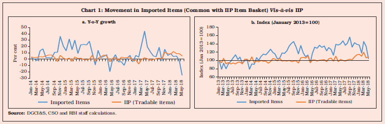ΔIIPt-1 is the growth of the manufacturing component of IIP with a one-period lag to account for the procurement of raw material inputs for final production; ΔUSDt is the month-on-month (MoM annualised) change in the nominal INR-USD exchange rate to factor in exchange rate effects embedded in imported inputs (ΔUSDt > 0 implies depreciation, and ΔUSDt < 0 represent appreciation). A dummy variable DummytD is used to capture the possible supply chain disruptions post-demonetisation and pre-GST implementation takes the value 1 from November 2016 to September 2017 and 0 otherwise20. The other dummy variable DummytPost takes value of 1 from October 2017 to May 2018, invigorates possible state of supply chain in post GST period. πwt-1 is non-food manufacturing component of the wholesale price index (WPI) controls for domestic price conditions – if domestic prices are benign, they will discourage imports. ΔPit is the year-on-year (YoY) growth of final goods produced by the ith target industry. Following the Arellano–Bond approach to estimation by the generalised method of moments (GMM), the dynamic panel regression yields the following results (Table 1). These results suggest that there is an adaptive process underway as imported inputs enter the domestic production process, as evident in the significance of the lagged dependent terms. The significance of DummytD indicates that there is a structural upward shift in the recourse to imports during the period post demonetisation, pointing to a regime change in which reliance on imported inputs increased significantly. On the other hand, the dummy for post GST period, exhibit negative significant coefficient indicating gradual normalisation in imports. The demand for imports is essentially being driven up by domestic demand represented by the growth of final products – as domestic production goes up in response to demand, the procurement of raw material inputs from abroad increases, given the constraints on domestic availability. Exchange rate changes work to deter import intensity, as expected, but only at the margin, as evident in the relatively small size of the coefficient on the exchange rate term. Domestic inflation works in tandem with the exchange rate – if inflation in India goes up, it incentivises recourse to cheaper imports. Table 1: Parameter Estimates of Dynamic Panel Regression   Coefficients SE 1 2 3 Import intensityt-1 (Iit-1) 0.412*** 0.040 Import intensityt-2 (Iit-2) 0.322*** 0.024 Dummy-D (DummytD) 0.181*** 0.090 Dummy – Post (DummytPost) -0.060** 0.024 Industry Growth (ΔPit) 0.004* 0.002 IIP Mfg growtht-1 (ΔIIPt-1) 0.038*** 0.021 INR-USD (ΔUSDt) -0.002** 0.001 WPI NFMP (πwt-1) 0.008* 0.003 Sargan test of over-identifying restrictions: (Prob > chi2) = 0.19. Note: ***, **, & *: Significant at 1 per cent, 5 per cent, and 10 per cent level of significance, respectively. Source: RBI staff estimates. In summary, import intensity of industrial raw materials used in manufacturing is influenced by domestic demand and cost conditions, whereas exchange rate depreciation plays a dampening role. The fact, however, that the dummy is significant from November 2016 up to September 2017 followed by reversal of sign of dummy in subsequent period, suggests that reverse import substitution effects was at best transient and ebbed gradually as industrial activity in India emerged out of its sluggish phase and regained its momentum.

3. Invisibles

II.6.11 Net invisibles – comprising net earnings from export of services, remittances and the net outgo of income payments (profits, dividends and interest payments) – recorded a double-digit growth in 2017-18. With a sizeable expansion in the merchandise trade gap, however, net invisibles could finance only 70 per cent of the merchandise trade deficit as compared with 87 per cent in the corresponding period of the previous year.

II.6.12 Among the major categories of services, export of travel services increased on the back of a significant jump in tourist arrivals during 2017-18 and increased per capita earnings from a year ago. Tourists from Bangladesh, the US and the UK accounted for about 45 per cent of total tourist arrivals. Introduction of policy measures to improve infrastructure facilities and revitalise heritage cities under the National Heritage City Development and Augmentation Yojana (HRIDAY) scheme in the Union Budget bode well for the travel and tourism sector. Meanwhile, higher travel payments by outbound Indian tourists also increased substantially during the year. Nevertheless, net receipts generated by travel services exceeded the level in the preceding year by about 30 per cent.

II.6.13 Despite a challenging global business environment in the IT sector, India’s software exports improved modestly, drawing support from a broad-based demand across industry verticals. Gradual diversification into advanced technological segments and moving up the value chain in IT supplemented the recovery process for major companies.

II.6.14 Inbound remittances by Indians working overseas – which were held back by lower international crude oil prices in the preceding year – recovered sharply in 2017-18 as income conditions in both AEs and the Gulf region improved. According to the World Bank (2018), global remittances are expected to be driven by a relatively stronger growth in the EU, Russian Federation and the US. Structural factors such as labour market adjustment in the Gulf countries and anti-immigration sentiment in many destination countries, however, may pose a downside risk going forward. Marginally higher net outgo on account of income payments reflected higher payments of profits and dividend on foreign investments.

4. Current Account Deficit

II.6.15 Notwithstanding buoyant net receipts from services exports and remittances, the CAD trebled during the year from its level a year ago, essentially due to the sharply higher merchandise trade deficit, and the worsening of both gross and net terms of trade (Chart II.6.5). In particular, the net terms of trade erosion caused by firming international commodity prices – especially of crude oil, gold and coal – is estimated to have widened the trade deficit by about 1.2 percentage points of GDP during 2017-18. During 2017-18, the CAD expanded to 1.9 per cent of GDP from 0.6 per cent a year ago, which remained far lower than the peak of 4.8 per cent attained in 2012-13. Furthermore, the CAD remained well within the norm of viability /sustainability (Chart II.6.6).

5. External Financing

II.6.16 Marking a shift from 2016-17, the funding mix of CAD was more diversified in 2017-18. Net investment inflows of foreign direct investment (FDI) and foreign portfolio investment (FPI) together amounting to US$ 52.4 billion and accounting for 57 per cent of net capital inflows, played a large role in external financing (Chart II.6.7).

II.6.17 Gross inflows of FDI to India increased during the year mainly due to higher flows into the communication services, retail and wholesale trade, financial services and computer services. In terms of sources, FDI inflows were concentrated mostly in Mauritius and Singapore that accounted for about 61 per cent of total equity investments. This was despite the phased implementation of an amended double taxation avoidance agreement with these countries effective from April 2017 to prevent evasion of taxes on income and capital gains. With the ongoing policy reforms in sectors ranging from single brand retail trading, civil aviation, real estate broking service and simplification of legal and regulatory system, India moved into the top 100 countries in the World Bank’s Ease of Doing Business global rankings. According to the UNCTAD’s Investment Trends Monitor (2018), India was the 10th largest recipient of global FDI in 2017 and remained the topmost destination for greenfield capital investment – even ahead of China and the US, if reckoned on an approval basis (FDI market intelligence 2017).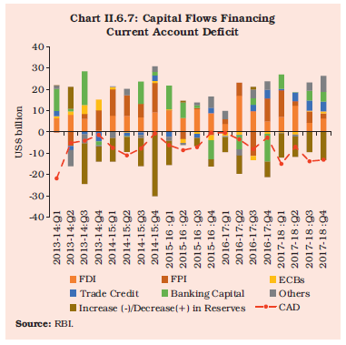

II.6.18 There was a substantial increase in FPI flows in 2017-18 from the preceding year, mainly driven by higher flows into the debt segment. FPI inflows in the debt segment were broadly resilient to risk-off effects of three Fed fund rate hikes in 2017-18. There were sell-offs around the world and in India in February and March though, as markets recalibrated expectations about the pace of normalisation of the US monetary policy. On the other hand, FPI into the equity segment slowed to almost half of its level in the preceding year amidst concerns about earnings growth, rising valuations and spillovers from monetary policy of systemic central banks. The introduction of the long-term capital gains (LTCG) tax in equity investments announced in the Union Budget on February 01, 2018 raised concerns, leading to net sell-off in February and the first half of March, slowing down the pace of FPI inflows. Investment in participatory notes (P-notes) slumped with regulatory tightening by the Securities and Exchange Board of India (SEBI), the application of a fee on each instrument issuance, and restrictions for FPIs in some derivative products. Foreign investors’ sustained interest in Indian capital markets, however, was reflected in a growing number of FPI registrations with the SEBI and net purchases in the equity market in March 2018. However, foreign portfolio investors withdrew US$ 9.1 billion on a net basis from the domestic capital market in 2018-19 (up to June 29), reflecting volatility in global financial markets.

II.6.19 A sharp increase in net inflows of short-term trade credit financed growing imports. In 2017-18, net inflows in the form of trade credit amounted to US$ 13.9 billion as compared with US$ 6.5 billion in 2016-17. Major imports with recourse to trade credit during the year included oil, gold and coal, which together accounted for nearly one-third of the total trade credit.

II.6.20 Although external commercial borrowings (ECBs) raised by domestic entities increased sharply, there were net outflows due to higher repayments. The Reserve Bank brought in restrictions on issuance of Masala bonds (rupee-denominated bonds issued abroad) by raising the minimum maturity period for issuances over and above US$ 50 million to five years and for those below US$ 50 million to three years. A cap on the all-in-cost ceiling was also put in place. Issuance of Masala bonds was also brought under the purview of the ECB approval process, thereby freeing up more space for investments by FPIs. ECBs in the form of rupee denominated bonds/ loans declined in 2017-18. About 33 per cent of the total ECB agreement amount (other than rupee denominated bonds/loans) was hedged during the period as compared with 41 per cent a year ago.

II.6.21 Net flows under non-resident deposit accounts witnessed a turnaround during the year despite a sharp moderation of deposits under Non-Resident (External) Rupee (NRE) accounts and Non-Resident Ordinary (NRO) accounts. This was essentially due to positive accretions of Foreign Currency Non-Resident (FCNR)(B) accounts as against a net outflow in the preceding year. The fall in deposits under NRE and NRO could be due to strengthening of the rupee during the year.

6. Vulnerability Indicators

II.6.22 At end-March 2018, India’s external debt expanded by US$ 58.4 billion from its level at end-March 2017. The rise was primarily due to an increase in portfolio investment in debt securities embedded in commercial borrowings, NRI deposits and short-term debt. Of the total external debt, 49.5 per cent was denominated in the US dollar, followed by the Indian rupee (35.8 per cent), the SDR (5.5 per cent), the Japanese Yen (4.8 per cent), the Euro (3.4 per cent) and others (1.0 per cent).

II.6.23 Notably, accretion to the external debt stock was modest and the average interest payments relative to external debt remained flat. The external debt-to-GDP ratio was the second lowest among the major EMEs, if compared with the 2016 level of external debt positions.

II.6.24 The movement in India’s external vulnerability indicators between end-March 2017 and end-March 2018 was somewhat mixed (Table II.6.1). The ratio of external debt to GDP increased marginally with the maturity profile of external debt tilted towards a shorter duration on both original and residual maturity bases. India’s foreign exchange reserves at end-March 2018 were more than adequate to meet short-term debt liabilities; nonetheless, these liabilities accounted for a larger share of foreign exchange reserves at end-March 2018 relative to March 2017. The foreign exchange reserves cover of imports declined between March 2017 and March 2018.

II.6.25 While strong capital inflows added to the stock of foreign liabilities, most of the increase was offset by the rise in stock of foreign assets largely reflecting the steep rise in foreign exchange reserves. As a result, India’s net foreign liabilities (i.e., net IIP) rose modestly and in terms of ratio to GDP, there has been a marginal decline at end-March 2018 over end-March 2017. The modest increase in net external liabilities is essentially a reflection of a modest and sustainable CAD.

II.6.26 To sum up, India’s external sector exhibited resilience despite the widening of the CAD on account of a surge in prices of major import commodities. Net inflow of foreign capital, however, exceeded the funding requirements of CAD which led to a significant build-up of reserves. The external sector outlook will be shaped by international commodity prices, the course of monetary policy in major AEs and the resulting cross-border spillovers, and the rising incidence of protectionism. Even though software exports could successfully withstand the challenging global business environment in the IT sector in 2017-18, further tightening of visa procedures in the US, the rise of automation and artificial intelligence, and competition from other markets including China can potentially impact export earnings. In this context, strengthening of domestic macroeconomic fundamentals holds the key to ensuring a viable external sector that is reasonably buffered against global shocks.

¹ A2 plus FL includes all paid out costs such as expenses on hired labour, machines, rent paid for leased land, seeds, fertilisers, irrigation charges, depreciation as well as imputed value of family labour.

² Rath, N. (2008), “Implications of the Loan Waiver for Rural Credit Institutions”, Economic and Political Weekly, June 14. EPW Research Foundation (2008), “The Loan Waiver Scheme”, Economic and Political Weekly, March 15.

³ In mining, stripping ratio or strip ratio refers to the ratio of the volume of overburden (or waste material) required to be handled in order to extract some tonnage of ore.

⁴ As regards CSO’s benchmark indicator for trade, the indicator has changed with the introduction of the GST - from actual sales tax collections to an estimated value using three approaches: (a) sales tax collection from products outside the purview of GST (like petroleum products); (b) regression of sales tax on value of output of commodity producing sectors; and (c) nominal growth in output of commodity producing sectors that are taxed. Information pertaining to these estimates are not yet available.

⁵ Headline inflation is measured by year-on-year changes in the all-India Consumer Price Index-Combined (CPI-C) (Rural + Urban) with base year: 2012=100 released by the Central Statistics Office (CSO), Ministry of Statistics and Programme Implementation, Government of India.

⁶ Patra et al, (2014) “Post-Global Crisis Inflation Dynamics in India: What has Changed?” in India Policy Forum 2013-14 provides a review of this literature.

⁷ Emerging and developing Asia includes 30 countries, the major ones being China, India, Indonesia, Malaysia, Thailand, Bangladesh, Bhutan, Sri Lanka, Philippines, Myanmar and Nepal.

⁸ Eleven Asian economies include six inflation targeters – India, Indonesia, Philippines, South Korea, Thailand and Japan, and the remaining non inflation targeters – China, Sri Lanka, Pakistan, Malaysia and Singapore.

⁹ When independent variables are not strictly exogenous and are correlated with their past, a dynamic panel model is considered to be appropriate. An Arellano-Bond dynamic panel using GMM in first difference of the regressors corrects for endogeneity, autocorrelation and deficiencies of the fixed effect panel regression. Arellano-Bover/Blundell-Bond, which is an augmented version of Arellano-Bond, allows for more instrumental variables, generally leading to an improved efficiency of the model.

¹⁰ Data are sourced from IMF’s World Economic Outlook (WEO) and International Financial Statistics (IFS), World Bank, CEIC and Bloomberg. The output gap for Asian economies is calculated using Hodrick-Prescott (HP) filter, while for advanced economies they are taken from WEO.

¹¹ Coefficients and Z-values correspond to robust standard errors. Arellano-Bond tests for zero autocorrelation in first-differenced errors confirmed the robustness of the models.

¹² In line with the budget proposal, the government fixed the MSPs for kharif crops on July 4, 2018, which were at least 1.5 times of A2+FL costs.

¹³ Besides wheat and paddy where procurement volumes are significant, some procurement also happens in the case of pulses and oilseeds by National Agricultural Cooperative Marketing Federation of India (NAFED) and Food Corporation of India (FCI) since 2016; and cotton and jute by the Cotton Corporation of India (CCI) and Jute Corporation of India (JCI); while several states also undertake procurement for release through the Public Distribution System (PDS) of items such as soyabeans in Madhya Pradesh, maize and ragi in Karnataka, jowar in Maharashtra and pulses in Tamil Nadu.

¹⁴ ‘Moneyness’ refers to the characteristic of an asset to convert readily into liquidity at a low or zero transaction cost.

¹⁵ Include volumes of real time gross settlement (RTGS), electronic funds transfer/national electronic funds transfer (EFT/NEFT), cheque truncation system (CTS), electronic clearing system (ECS), immediate payment service (IMPS), cards usage at point of sale, prepaid payment instruments (PPIs), mobile banking transactions and national automated clearing house (NACH).

¹⁶ The discussion on central government finances for 2017-18 is based on Provisional Accounts (PA) and for 2018-19 on Budget Estimates (BE).

* As per the Finance Act, 2018.

¹⁷ State Finances: A Study of Budgets 2017-18 and 2018-19, Reserve Bank of India, July 2018.

¹⁸ Gross income elasticity of global trade is measured as the ratio of the average growth rate of imports of goods to average GDP growth.

¹⁹ Monthly data on commodity level imports and segment-wise industrial production in the IIP from January 2013 to May 2018 were mapped for extracting common items. Import data were deflated by corresponding wholesale price indices (WPI). Both real imports and the IIP elements were indexed (January 2013 at 100).

²⁰ The dummy variable has been altered to take into account different end points starting from June to September 2017 to validate the robustness of the results.