The macroeconomic environment in 2014-15 was marked by a modest pick-up in activity amidst building internal
and external stability, against the backdrop of a tepid and multi-speed global recovery across regions. Going forward,
the economy needs to grapple with significant challenges in the path towards realising its potential and sustaining
the growth process. Importantly, structural constraints to growth and asset quality concerns need to be addressed
sooner than later.
II.1 THE REAL ECONOMY
II.1.1 In January 2015, the Central Statistics
Office (CSO) released a new series on India’s
national accounts. The distinguishing features of
the new series are: (i) updating the base year from
2004-05 to 2011-12; (ii) improved coverage of
corporate activity by (a) using the MCA 21
database1 of the Ministry of Corporate Affairs, (b)
employing value-based indicators such as sales
tax collections in conjunction with volume-based
indicators such as industrial production, and (c) use
of results from the latest surveys, including on
activity in the unorganised sector; and (iii)
methodological changes such as shifting from the ‘establishment’ to the ‘enterprise’ approach for
estimating value added in mining and manufacturing.
In line with international practices, GDP at market
prices will henceforth be the headline measure for
output. Gross value added (GVA) at basic prices
will measure activity from the supply side instead
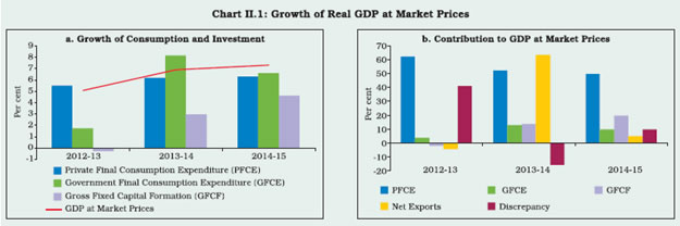
of GDP at factor cost. In terms of the new series,
real activity (at market prices) picked up in 2014-15,
rising by 7.3 per cent on top of a growth of 6.9 per
cent in 2013-14 (Chart II.1). The firming up of
growth during 2014-15 was driven mainly by private
consumption and supported by fixed investment,
even as government consumption and net exports
slackened considerably.
 II.1.2 From the supply side, the quickening of
activity in 2014-15 was largely led by industry and
services (Chart II.2). Within industry, higher growth
was observed in manufacturing and electricity
generation. The share of manufacturing was
augmented by trading activity of constituent entities
which formed part of services in the old series. In
the services sector, ‘financial, real estate, and
professional services’ as well as construction were
the primary drivers. On the other hand, the
agriculture sector lost momentum, adversely
impacted by the deficient southwest monsoon
(SWM) which affected kharif sowing and by
unseasonal rains and hailstorms at the time of rabi
harvesting.
II.1.3 Thus, in terms of the new series, India
emerged among the fastest growing economies in
the world, notwithstanding the still sluggish global
economy which dragged down the contribution of
net exports to growth in 2014-15.
Saving and Investment
II.1.4 In 2013-14, the gross domestic saving rate
declined for the second consecutive year to 30 per
cent of gross national disposable income (GNDI)
(Table II.1) This largely reflected the reduction in
the saving rate of households on account of a
decline in physical assets as well as in valuables.
On the other hand, household financial saving
gained from returns turning attractive with the moderation in inflation as well as the pick-up in
economic activity. For 2014-15, CSO has not yet
released its estimates of gross saving. However,
in terms of the Reserve Bank’s preliminary
estimates, household financial saving is placed at
7.5 per cent of GNDI in 2014-15, up from 7.3
per cent in 2013-14.
| Table II.1: Gross Saving (As a ratio of GNDI) |
| (Per cent) |
| Item |
2011-12 |
2012-13 |
2013-14 |
| 1 |
2 |
3 |
4 |
| 1 |
Gross Savings |
33.0 |
31.1 |
30.0 |
| |
1.1 Non-financial Corporations |
9.7 |
9.6 |
10.3 |
| |
1.1.1 Public non-financial corporations |
1.4 |
1.2 |
1.0 |
| |
1.1.2 Private non-financial corporations |
8.3 |
8.4 |
9.3 |
| |
1.2 Financial Corporations |
2.9 |
3.1 |
2.8 |
| |
1.2.1 Public financial corporations |
1.8 |
1.7 |
1.5 |
| |
1.2.2 Private financial corporations |
1.1 |
1.4 |
1.3 |
| |
1.3 General Government |
-1.8 |
-1.3 |
-1.0 |
| |
1.4 Household sector |
22.2 |
19.7 |
17.8 |
| |
1.4.1 Net financial saving |
7.1 |
6.8* |
7.1* |
| |
1.4.2 Saving in physical assets |
14.8 |
12.6 |
10.4 |
| |
1.4.3 Saving in the form of valuables |
0.4 |
0.4 |
0.3 |
Note: Net financial saving of the household sector is obtained as the difference between change in financial assets and change in financial liabilities.
Source: Central Statistics Office.
*: As per Reserve Bank’s latest estimates, household financial saving for 2012-13 and 2013-14 are 7.0 per cent and 7.3 per cent, respectively, of GNDI. |
II.1.5 As regards the saving rate of the private
corporate sector, non-financial corporations posted
a near-steady improvement since 2011-12, i.e.,
since the new series is available, but it appears that
this increase may not have sustained in 2014-15.
Private financial corporations, on the other hand,
underwent some erosion in saving rates in 2013-14,
partly reflecting the slowdown in the growth of
operating profits of private sector banks. Available
indicators suggest that this has been recouped in
2014-15.
II.1.6 The ongoing reduction in ‘dissaving’ of the
general government boosted the gross national
saving rate in 2013-14. With the perseverance of
fiscal consolidation, especially by the centre, the
decline in the dissaving of the government sector
has likely continued into 2014-15. There was,
however, a decline in the saving rate of the public
financial (including public sector banks) and nonfinancial corporations in 2013-14. In case of public
sector banks, there was a decline in profit after tax
during 2014-15.
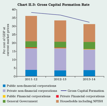
II.1.7 The investment rate (gross capital
formation as a proportion to GDP at current market
prices) declined in 2012-13 and 2013-14, largely
reflecting the slackening in the non-financial
corporations’ investment rate on account of weak
domestic and external demand and other structural
factors such as delay in land acquisition and
environment clearances, weak business confidence
and policy uncertainties. The household sector’s
investment rate also declined in 2012-13 and
2013-14. The improvement in general government
investment in 2013-14 did, however, provide some
offset (Chart II.3).
II.1.8 Viewed in conjunction with other indicators
of investment activity such as stalled projects, capital goods imports/production and capex
spending, the decline in the private investment
intention appears to have become more pronounced
in 2014-15 relative to the preceding year. As per
the Reserve Bank’s data on new projects which
were sanctioned financial assistance by banks/
financial institutions (FIs) or funded through external
commercial borrowings (ECBs)/foreign currency
convertible bonds (FCCBs)/domestic capital market
issuance, investment intentions for such projects
aggregated to ₹1,459 billion during 2014-15 as
against ₹2,081 billion in the previous year. A
turnaround in the investment demand cycle,
therefore, assumes critical importance to steer the
economy on to a sustainable high growth trajectory.
The recent experience suggests that a strong stepup
in public investment may be required to dispel
the inertia constraining private investment and to
crowd it in, given the robust business sentiment.
Key to this effort will be putting stranded investments
in stalled projects back to work while ensuring the
availability of key inputs such as power, land
(especially for roads) and skilled labour. Steadfast
implementation of structural reforms like the goods
and services tax (GST) is also required to
reinvigorate productivity and competitiveness.
 Agriculture
II.1.9 The vagaries of the monsoon were in full
play during 2014-15. The likelihood of El Nino
emerging, was initially placed high, but it eventually
did not materialise. Nevertheless, delay, deficiency,
and unevenness in rainfall during the SWM season
led to a decline in the production of most kharif
crops. The deficient SWM did not replenish soil
moisture adequately and, in addition, the northeast
monsoon (NEM) also turned deficient. With the
production of most rabi crops estimated lower, the
initial hope that a good rabi harvest could make up
for the kharif losses was belied. At the end of the
seasons, the SWM turned 12 per cent below the
long period average (LPA) and the NEM 33 per cent
below the LPA. In addition to under-replenishment
of reservoirs and intermittent dry halts, a bigger
blow to rabi crops, mainly to wheat, came in the
form of unseasonal rainfall and hailstorms during
late February and early March 2015. As per the
fourth advance estimates of the Ministry of
Agriculture released on August 17, 2015, the total
foodgrains production declined by 4.6 per cent.
Similarly, the production of oilseeds and cotton
declined by 18.5 per cent and 1.2 per cent
respectively, though that of sugarcane increased by 2.0 per cent. The impact of a decline in the
volume of foodgrains production to 252.7 million
tonnes from 265.0 million tonnes a year ago may,
however, be mitigated by the availability of food
stock buffers of 55.6 million tonnes (end-July 2015),
which is much higher than the buffer norm which
varies between 21.0-41.1 million tonnes.
II.1.10 For the 2015 SWM season, the India
Meteorological Department (IMD) has forecast
precipitation at 88 per cent of the LPA in June 2015,
and retained the same forecast in August 2015 with
a higher likelihood of El Nino effect intensifying
during the season2. Though delayed in arrival, the
rainfall was in excess in June barring the last week
when a dry spell set in and continued till mid-July,
limiting the season’s precipitation to 9 per cent
below LPA so far (August 19, 2015). Better rainfall
in June augmented sowing under most kharif crops
vis-à-vis last year. In view of these developments,
the prospects of kharif harvest 2015 could be
expected better notwithstanding the persisting risks
to supply shortfalls and likely inflation pressures
given the unpredictability of SWM during the
remaining part of the season, alongside the need
for reappraisal of the degree of weather proofing of
Indian agriculture in the context of monsoon
vagaries (Box II.1).
Box II.1
How Monsoon Proof is Indian Agriculture?
Historically, agricultural failures in India have often been
associated with deficient south west monsoons (SWM). The
SWM which constitutes 75-80 per cent of total rainfall received
in India, coincides with kharif sowing and is vital for
replenishment of ground water, soil moisture and reservoirs
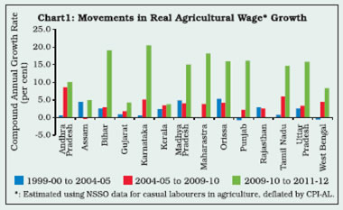
and thus crucial for a good rabi harvest as well. Visual
observation of trend growth rates of agriculture seems to
suggest resilience at least in some bad monsoon years
(Chart 1).
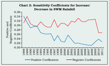
Empirical analysis of positive and negative SWM shocks
suggests that during 1988-2012, the impact of variations in
SWM is statistically significant for agricultural output, but it is much less than that of variations in net sown area (Chart 2).
The absence of multicollinearity between rainfall and sown
area is validated by variance inflation factor (VIF).
 Clearly, Indian agriculture is yet to become fully weather
proof and public policy interventions to insulate crop
production from monsoon shocks is an imperative. Saturation
of land use and exhaustion of economies of scale can be
halted by multi-pronged strategies covering, inter alia, credit,
capital and machinery, technology, research and
development, use of improved and hybrid seeds, irrigation
and water management, and land reclamation including in
arid and semi-arid areas while more vigorously pursuing the scheme of extending the green revolution in the east. A
diversified approach to agricultural development with
emphasis on livestock, fishery, forestry and logging will also
buffer agricultural output from SWM variations, provided it
is pursued in the overall context of food and nutritional
security.
Contingency plans put in place during 2009-10 in the face of
a 22 per cent shortfall in SWM warrant careful consideration
for replication. The provision of quality and short duration
seeds, agricultural inputs, an active rabi campaign and an
action plan for the next cropping season, media telecasting
and awareness campaigns, enhanced availability of funds
under centrally sponsored programmes, and additional diesel
subsidy for irrigation served well, bringing home the point that
the impact of adverse monsoon shocks can be ameliorated
by pro-active policy measures.
References:
Aggarwal P.K. et al. (2009), ‘Vulnerability of Indian Agriculture
to Climate Change: Current State of Knowledge’ available at
http://www.moef.nic.in
RBI Bulletin (2015), ‘Monsoon and Indian Agriculture –
Conjoined or Decoupled?’, May.
Industry
II.1.11 Industrial production turned around from
the contraction recorded in 2013-14 and posted a
growth of 2.8 per cent during 2014-15. The
production of consumer durables continued to
shrink as in the previous year, especially telephone
instruments, including mobile phones which was
due to the one-off closure of Nokia’s manufacturing
unit in Chennai in November 2014. Excluding this
category, industrial production would have risen by
5.3 per cent during 2014-15 (Chart II.4).
II.1.12 Higher production of basic metals, electricity
and capital goods drove up the index of industrial
production (IIP) growth during 2014-15. In terms of
the use-based classification, the production of basic
and capital goods accelerated, while that of
intermediate goods decelerated and the output of
consumer goods contracted (Table II.2).
| Table II.2: Index of Industrial Production |
| (Per cent) |
| Industry Group |
Weight in IIP |
Growth Rate |
| 2011-12 |
2012-13 |
2013-14 |
2014-15 |
April-June 2015-16P |
| 1 |
2 |
3 |
4 |
5 |
6 |
7 |
| Overall IIP |
100.0 |
2.9 |
1.1 |
-0.1 |
2.8 |
3.2 |
| Mining |
14.2 |
-2.0 |
-2.3 |
-0.6 |
1.5 |
0.7 |
| Manufacturing |
75.5 |
3.0 |
1.3 |
-0.8 |
2.3 |
3.6 |
| Electricity |
10.3 |
8.2 |
4.0 |
6.1 |
8.4 |
2.3 |
| Use-Based |
|
|
|
|
|
|
| Basic Goods |
45.7 |
5.5 |
2.5 |
2.1 |
7.0 |
4.7 |
| Capital Goods |
8.8 |
-4.0 |
-6.0 |
-3.6 |
6.4 |
1.5 |
| Intermediate Goods |
15.7 |
-0.6 |
1.6 |
3.1 |
1.7 |
1.6 |
| Consumer Goods |
29.8 |
4.4 |
2.4 |
-2.8 |
-3.4 |
2.4 |
| Consumer Durables |
8.5 |
2.6 |
2.0 |
-12.2 |
-12.6 |
3.7 |
| Consumer Non-durables |
21.3 |
5.9 |
2.8 |
4.8 |
2.8 |
1.6 |
| Source: Central Statistics Office.
P: Provisional |
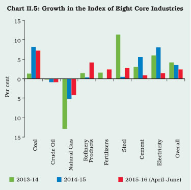
II.1.13 Mining activity recovered during 2014-15
from a three-year slump, buoyed by a sharp increase in the production of coal (Chart II.5). Among other
items within the mining sector, the production of
crude oil declined on account of ageing oil fields and
delay in the execution of new oil field projects. Also,
contraction in the production of natural gas from the
KG-D6 block affected natural gas production during
2014-15 as in the previous three years. Electricity
generation registered its highest growth in the last
two decades during 2014-15, facilitated by improved
coal supply and higher capacity addition of 22,566
MW (as against a target of 17,830 MW), which is
the highest ever achieved in a single year. Capacity
addition, coupled with higher generation and
improved transmission capacity resulted in a
considerable reduction in power shortage from a
level of 7 to 11 per cent during the last two decades
to a record low of only 3.6 per cent during 2014-15.
The plant load factor (PLF) in the thermal power
sector was largely sustained in 2014-15. However,
there has been some slippage in the PLF in the first
quarter of 2015-16.
 II.1.14 Weakness in consumer spending, sluggish
investment activity and poor external demand operated as drags on manufacturing activity during
2014-15. Within the manufacturing sector, exportoriented
industries like textiles, wearing apparels
and refined petroleum products decelerated. On
the other hand, capital goods industries like
machinery and equipment and electrical machinery registered improved growth. Revival in the
production of capital goods after three years of
contraction signals improved prospects for
investment demand going forward. During April-
June 2015, however, the growth in IIP decelerated
mainly on account of a sluggish performance in
capital goods, electricity and food products.
Services
II.1.15 The services sector is estimated to have
grown by 9.4 per cent during 2014-15 mainly driven
by ‘financial, real estate and professional services’
and construction sector. As for 2015-16, available
data on lead indicators of services sector including
commercial/passenger vehicles sales, air passenger
traffic, port and international air cargo, show an
improvement over the corresponding period last
year. However, railway freight traffic, domestic air
cargo, tourist arrivals, cement production and steel
consumption - which provide lead indications of
construction activity- show moderation. During
2014-15, purchasing managers index (PMI) for
services remained in an expansionary mode since
May 2014, though the rate of expansion was at a
slower pace in ensuing months. However, PMI
services contracted in May-June 2015 on account
of a decline in both output and new orders though
it expanded marginally in July 2015. Also, given the
drag emanating from fiscal consolidation by central
and state governments on total spending, ‘public
administration, defence and other services’ may not
serve as a durable growth driver, going forward.
Employment Generation
II.1.16 Quarterly employment surveys conducted
by the Labour Bureau for select export-oriented
sectors reveal that the rate of employment
generation in these sectors picked up in 2013 and
2014, after a significant decline in 2012. However, the pace of employment generation is yet to recover
to its pre-2010 level. Information technologybusiness
process outsourcing (IT-BPO) and textiles
continue to be the key export oriented sectors
generating large employment from 2009 to 2014.
Infrastructure
II.1.17 The growth of production in core industries
(coal, crude oil, natural gas, refinery products,
fertilisers, steel, cement and electricity) moderated
during 2014-15 (Chart II.5) and remained sluggish
during April-June 2015. Structural constraints have
resulted in a persistent decline in the production of
natural gas, crude oil and fertilisers. The growth of
the steel industry was affected by the fall in global
prices of steel and the resultant increase in steel
imports. On the other hand, the coal sector’s
impressive growth performance during 2014-15
benefitted from several efficiency enhancing
measures taken by the government for Coal India
Limited (CIL), like use of mass production
technologies, rationalisation of linkages from coal
sources to end-users, coordinated efforts with
railways for speedy evacuation of coal and shifting
to underground mines.
II.1.18 As on mid-August 2015, the government’s
Project Monitoring Group (PMG) has received
proposals for 675 projects (₹10 billion and above
or any other critical projects in sectors such as
infrastructure, manufacturing and power) with an
estimated project cost of ₹28.8 trillion for its
consideration. Out of these, 291 projects worth ₹9.9
trillion were cleared by the PMG with the majority
of projects pertaining to the power sector, followed
by coal, road and petroleum sectors. However, the
impact of government initiatives is yet to be felt in
terms of the revival of central sector infrastructure
projects (₹1.5 billion and above) monitored by the Ministry of Statistics and Programme Implementation
(MoSPI) (Table II.3).
|
| Table II.3: Status of Projects |
| Central Sector Infrastructure Projects |
| Period |
Total No. of Projects |
No. of Delayed Projects |
Value of Delayed Projects (₹ billion) |
No. of projects without DOC |
Value of projects without DOC (₹ billion) |
| 1 |
2 |
3 |
4 |
5 |
6 |
| May-15 |
766 |
237 |
4,826 |
371 |
2,470 |
| Mar-15 |
751 |
328 |
5,752 |
264 |
1,531 |
| Dec-14 |
738 |
315 |
4,961 |
266 |
1,475 |
| Sep-14 |
750 |
312 |
5,504 |
302 |
1,730 |
| Jun-14 |
729 |
290 |
4,975 |
300 |
1,805 |
Source: Infrastructure and Project Monitoring Division, MoSPI, Government of India (GoI).
DOC: Date of Commissioning. |
II.1.19 While investment through the public-private
partnership (PPP) mode was the highest in India
during 2008 to 2012 as per the World Bank’s
database3, thereafter the private participation in
prime infrastructure projects in roads and ports
decreased sharply. The focus of the government
on construction of highways through the publicly
funded engineering, procurement and construction
(EPC) mode is reflected in a marginal improvement
in road construction activity in 2014-15 vis-à-vis
2013-14 (Chart II.6).
II.1.20 Spectrum auctions in March 2015 elicited
vibrant bidding for all the four bands (1800 MHz,
900 MHz, 2100 MHz, and 800 MHz). This is the first
time that spectrum has been offered simultaneously
in all the four bands (Table II.4).
| Table II.4: Spectrum Auction |
Year |
Revenue Realisation (₹ billion) |
1 |
2 |
2010 |
1062.62 |
2012 |
94.07 |
2013 |
36.39 |
2014 |
611.61 |
2015 |
1098.75 |
| Source: Ministry of Information & Communication Technology, GoI. |
II.1.21 The government initiated a number of
structural reforms in the recent period to boost the
infrastructure sector: the passing of the Coal Mines
(Special Provisions) Act, 2015; auctioning of coal
mines; hike in tariffs on iron and steel; adoption of
the plug-and-play mode of project execution for
mega power projects; allowing foreign direct
investment up to 100 per cent in railway infrastructure; the proposed National Investment and
Infrastructure Fund; tax free infrastructure bonds
for projects in the rail, road and irrigation sectors
and increased plan outlays for roads and railways.
II.1.22 In order to give a direct thrust to
infrastructure investment, the government has
stepped in to boost public spending in infrastructure
by ₹700 billion in 2015-16. These efforts are also
expected to crowd in private participation. Going
forward, the government’s decision to award
new projects only after obtaining the requisite
clearances and linkages could catalyse the pace
of infrastructure project completion.
II.2 PRICE SITUATION
II.2.1 The year 2014-15 marked a turning point
in the evolution of price-cost dynamics in India. In
January 2014, the stance of monetary policy was
anchored to a path of disinflation that would take
inflation (measured in terms of y-o-y changes in
the all India consumer price index (combined) or
CPI-C, base 2010 =100) down from 8.6 per cent
to below 8 per cent by January 2015 and to below
6 per cent by January 2016. This stance was
backed by policy rate increases of 25 basis points
each in September 2013, October 2013 and
January 2014. Although unseasonal food price
spikes owing to weather-related transportation
disruptions in north India kept inflation stubbornly
high till July 2014, steadfast perseverance with the
anti-inflationary monetary policy allowed rate
increases in the second half of 2013-14 to feed
through into the economy. Aided by a range of
supply management strategies and a dramatic
plunge in international commodity prices4 by 28
per cent between September 2014 and February
2015, inflation persistence (near double digit CPI
inflation for six consecutive years) was finally
broken and headline inflation started easing from
August 2014. The abatement in food price
pressures contributed 76 per cent to the decline in
inflation between July and November 2014. By April
2015, it had declined to 4.9 per cent measured by
the new CPI series (base 2012=100), thus
confirming that disinflation was getting entrenched.
Notwithstanding an uptick in June 2015 to 5.4 per
cent, largely reflecting fuel price adjustments and
short-term food price pressures, inflation moderated
significantly to 3.8 per cent in July 2015. Importantly,
inflation excluding food and fuel almost halved from
8.3 per cent in May 2014 to 4.2 per cent in March 2015, providing abiding momentum to the
disinflation process. However, this moved
significantly up to 5.0 per cent in June 2015 before
falling to 4.5 per cent in July 2015. By December
2014, households’ inflation expectations (both
three months ahead and one-year ahead), which
had been ruling in double digits persistently since
September 2009, eased to single digit.
II.2.2 Average inflation at 5.9 per cent during
2014-15 turned out to be significantly lower than
9.5 per cent a year ago (Chart II.7). Intra-year
movements in inflation during 2014-15, however,
exhibited three distinct phases – first, weatherrelated
vegetable price pressures till August;
second, the subsequent fall in food prices and
pass-through of declining global commodity prices
into food, fuel and services prices, resulting in a
major shift in the inflation trajectory that took
inflation down to an intra-year low of 3.3 per cent
in November 2014; and finally the reversal of
favourable base effect, which pushed inflation up to 5.3 per cent in March 2015. Significantly, even
as inflation moved up during December 2014 -
February 2015, the month-on-month increase in
prices remained moderate or negative, attesting
to the sustained abatement of inflation risks.
Drivers of CPI Inflation
II.2.3 All the three major constituent groups of
CPI - food, fuel and categories excluding food and
fuel - contributed to a decline in headline inflation,
reflecting improvement in supply conditions and
the ebbing of inflation momentum (Chart II.8), with
the largest impact emanating from the food
component. Fuel group’s contribution to inflation
remained marginal, reflective of its relatively lower
weight and declining frequency of changes in
administered prices of non-transport fuel items.
The fall in inflation, excluding food and fuel, was
facilitated by the anti-inflationary monetary policy
stance as inflation in most of its sub-components
edged down.
Food Inflation
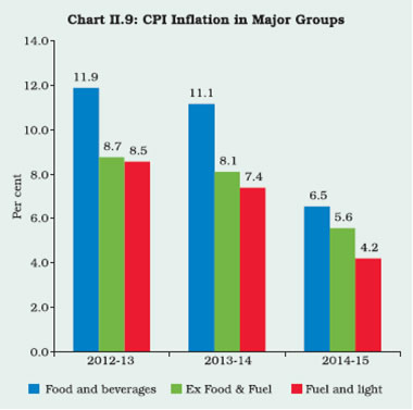
II.2.4 The wedge between inflation in food and
non-food groups narrowed considerably during
2014-15 (Chart II.9). Two major groups - cereals
and vegetables - together accounted for almost
80 per cent of the decline in average food price
inflation during the year. Cereals’ inflation declined
partly on account of the lower order of revision in
minimum support prices (MSPs) in 2014-15 (Table
II.5) and active supply management under the public distribution system (PDS), including the
open market sale of wheat. Vegetable prices
shrugged off bouts of weather-related volatility in
H1 of 2014-15 and declined relatively faster in H2
of 2014-15 with policy actions taken to discourage
stockpiling, and bringing vegetables under the
Essential Commodities Act (ECA). Sugar prices
moderated in tandem with global prices, but
protein-rich items (eggs, fish, meat, milk and
pulses) exhibited downward rigidity in inflation,
reflecting structural mismatches between demand
and supply.
| Table II.5: Minimum Support Prices of Food
Grains (₹ per quintal) |
| Commodity |
2012-13 |
2013-14 |
2014-15 |
2015-16 |
| 1 |
2 |
3 |
4 |
5 |
| Paddy (Common) |
1,250 |
1,310 |
1,360 |
1,410 |
| Wheat |
1,350 |
1,400 |
1,450 |
- |
| Gram |
3,000 |
3,100 |
3,175 |
- |
| Arhar (Tur) |
3,850 |
4,300 |
4,350 |
4,425 |
| Moong |
4,400 |
4,500 |
4,600 |
4,650 |
| Urad |
4,300 |
4,300 |
4,350 |
4,425 |
| Source: DAC, Ministry of Agriculture & Farmers Welfare. |
II.2.5 A number of policy initiatives were taken
to improve both supply chain and post-harvest
crop management. These included issuing
advisories to states to enable free movement of
fruits and vegetables by delisting them from the
Agricultural Produce Marketing Committee
(APMC) Act; bringing onions and potatoes under
the purview of ECA, thereby allowing state
governments to impose stock limits so as to deal
with cartelisation and hoarding and making
violation of stock limits a non-bailable offence.
Imposing a minimum export price (MEP) of US$
450 per metric tonne (MT) for potatoes with effect
from June 26, 2014 and US$ 300 per MT for onions
with effect from August 21, 2014 also helped in
maintaining domestic supplies of these perishable
items.
Fuel Group Inflation
II.2.6 From August 2014, crude oil prices fell but
the full pass-through of this decline was impeded
by lingering under-recoveries of the oil marketing
companies (OMCs) (Table II.6). Further, the
government increased the excise duty on petrol
and diesel cumulatively by ₹7.75 per litre for petrol and ₹6.50 per litre for diesel during November
2014 - January 2015, which partially offset the
overall fall in prices. In case of coal, Indian prices
have historically remained substantially lower than
the global prices. Therefore, the decline in global
coal prices during 2014-15 resulted in bridging the
gap between global and domestic prices rather
than a fall in domestic prices. Since the CPI fuel
group includes a number of items, such as
electricity and kerosene whose prices are
administered, prices in this category remained
sticky (Chart II.10).
| Table II.6: Under-recoveries of
Oil Marketing Companies |
| (₹ billion) |
| Product |
2013-14 |
2014-15 |
| 1 |
2 |
3 |
| Diesel |
628 |
109 |
| PDS Kerosene |
306 |
248 |
| Domestic LPG |
465 |
366 |
| Total |
1,399 |
723 |
| Source: PPAC, Ministry of Petroleum & Natural Gas. |
Inflation Excluding Food and Fuel
II.2.7 Prices in respect of the transport and
communication sub-group declined in tandem with
softening of global crude oil prices. By the end of
the year, the transport and communication
category contributed negatively to inflation (Chart
II.11). Also, housing inflation showed a much more
significant moderation under the new series (base
2012=100) partly on account of methodological
improvements, which included doubling the
sample size for collection of rentals data from
6,684 rented dwellings in the old series to 13,368
in the revised series. Inflation in services
components, such as health, education and
household requisites declined, reflecting a
slowdown in wage growth.
Rural Wage Growth Moderated
II.2.8 Input cost pressures from fuel, farm inputs
and rural wages ebbed significantly during 2014-
15. After the high and unprecedented rise in rural
wages during 2007-08 to 2012-13, the recent
slowdown in wage growth has evoked academic and policy interest. Average wage growth, as per
the new wage series, for November 2014 to May
2015, remained at 3.9 per cent for agricultural and
5.7 per cent for non-agricultural occupations,
respectively. This was substantially lower than the
annual average rate of 16 per cent for agricultural
occupations and 14 per cent for non-agricultural
occupations during the six-year period from 2007
to 2013. However, the role of productivity will have
to be examined carefully while assessing the
durability of the impact of the changes in wage
growth on inflation (Box II.2).
Box II.2
Wage Growth and Rural Inflation – Are They Related?
An increase in rural wages can influence prices, both by
increasing demand and pushing up the cost of production.
On the other hand, wage growth in itself could respond to
high price increases, particularly food price increases. The
wage-inflation nexus also works through productivity - as
labour productivity increases, wages rise. An increase in
labour productivity will reduce unit labour cost, which is the
average cost of labour per unit of output (usually calculated
as the ratio of total labour costs to real output) and therefore,
it will be possible to pay a higher wage without an increase
in final output price. On the other hand, if wage increases
are unaccompanied by productivity increases, rise in unit
labour costs will lead to further increase in output prices and
hence inflation. This dynamics is more complex in a regional
perspective, where there is large heterogeneity in product
and labour markets.
A comparison between agricultural labour productivity and
agricultural wages at the all-India level as well as for major
states is insightful. Real wage growth, i.e., growth in
agricultural wages adjusted for CPI - agricultural labourers
(AL) inflation, remained moderate during 1999-00 to 2009-
10. Subsequently, it went up sharply during 2009-10 to
2011-12 (Chart 1). This trend was broad-based and
observed in major agricultural states like Bihar, Maharashtra,
Madhya Pradesh, Tamil Nadu and Uttar Pradesh.
 Agricultural labour productivity declined in some states
over the period from 1999-2000 to 2004-05, but went up
subsequently during the period 2009-10 to 2011-12 at the
all-India level as well as for major states (Chart 2). The
productivity improvement was partly contributed by a shift
in labour force from agricultural to non-agricultural
occupations, which led to a decline in the total number of
persons engaged in agriculture in 2011-12 vis-à-vis 2004-
05. Thus, the sharp increase in real wages in recent years
was partly offset by a rise in productivity. The impact of
rural wage increases on rural food prices was not as large
due to commensurate rise in productivity (Goyal and Baikar
2014). Post-2013, real wage growth declined in India
barring a few states like Madhya Pradesh, Uttar Pradesh,
Gujarat and Tamil Nadu. The fall in real wage growth is
mainly contributed by a fall in nominal wage growth.
References:
Dholakia, R.H., M. B. Pandya and P. Pateriya (2014), ‘Urban
– Rural Income Differential in Major States: Contribution of
Structural Factors’, WP No. 7, Indian Institute of Management,
Ahmedabad.
Goyal, A. and A.K. Baikar (2014), ‘Psychology, Cyclicality
or Social Programs: Rural Wage and Inflation Dynamics in
India’, WP, IGIDR, Mumbai.
Wholesale Price Inflation
II.2.9 Inflation measured by the wholesale price
index (WPI) declined significantly during 2014-15.
Since November 2014, wholesale prices have
moved into contraction [(-) 4.1 per cent in July
2015, y-o-y] (Chart II.12). Prices of non-food
manufactured products also contracted in July
2015 [(-) 1.4 per cent, y-o-y], indicating the extent
of slack in the economy as well as falling cost
pressures.
Global Commodity Prices and Supply Conditions
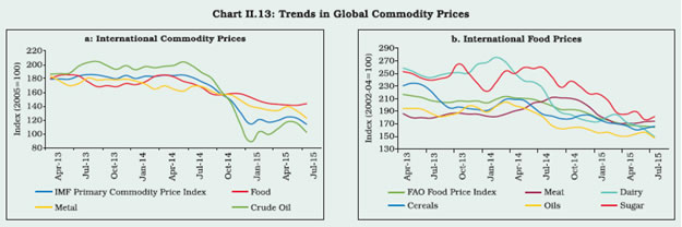
II.2.10 Global commodity prices declined sharply
amidst improved supply, large spare capacity and
weak demand conditions in 2014-15 (Chart II.13).
During the initial part of the year, crude oil prices
hardened on account of supply outages in Libya,
Nigeria and Syria. From August 2014, global
crude oil prices fell substantially, driven by
abundant supplies of North American shale oil
and the Organisation of Petroleum Exporting
Countries’ (OPEC) decision not to cut production
at its November 2014 meeting. Global crude oil
prices reached a trough of US$ 47 per barrel (Indian basket), marking a decline of 57 per cent
during June 2014 to January 2015. Though the
slow pace of global economic recovery has kept demand prospects weak, the International
Monetary Fund (IMF) estimated that lower
demand could account for only 20 to 35 per cent of the price decline between June and December
2014.
 II.2.11 Since January 2015, several factors, such
as falling oil rigs in the US, decline in stockpiles
and elevated geo-political tensions in the Middle
East rekindled upside risks to oil prices. Indian
basket prices firmed up to US$ 63.8 per barrel in
May 2015 but declined subsequently to US$ 49
per barrel by mid-August 2015 as supply prospects
improved with the clinching of the nuclear deal by Iran with the major world powers. Metal prices
edged down in 2014 aided by surplus supplies
and slowing demand conditions in emerging
economies, particularly in China.
II.2.12 Global food prices declined by 3.8 per cent
in 2014 as large accumulated stocks continued to
pull down international prices of commodities, such
as cereals, oils and sugar. The Food and Agriculture
Organisation (FAO), in its update of July 2015,
forecast that the world cereals production might
decline by 1.1 per cent in 2015 while exceptionally
high stocks were likely to compensate for the
production shortfall. During 2015 so far, prices have
continued to move downwards for almost all food
items, with large supplies and slow trading activity
as buyers are expecting a further fall in prices in
the coming months.
Revision in the CPI Base Year
II.2.13 In order to capture shifting consumption
pattern of households, the Central Statistics Office
(CSO) revised the base year of CPI to 2012 from
its earlier base of 2010, using the weighting pattern
from the latest consumer expenditure survey (CES),
2011-12 of the National Sample Survey Office (NSSO). Changing patterns of consumer
expenditure over the years are reflected in subcategory-
wise weights computed for the new CPI
series (Table II.7).
| Table II.7: Comparison of Weighting Diagrams–Previous and Revised CPI Series |
| (Per cent) |
| Sub-Categories |
Base Year: 2010 |
Base Year: 2012 |
| Rural |
Urban |
Combined |
Rural |
Urban |
Combined |
| 1 |
2 |
3 |
4 |
5 |
6 |
7 |
| Food and Beverages |
56.59 |
35.81 |
47.58 |
54.18 |
36.29 |
45.86 |
| Pan, Tobacco and Intoxicants |
2.72 |
1.34 |
2.13 |
3.26 |
1.36 |
2.38 |
| Clothing and Footwear |
5.36 |
3.91 |
4.73 |
7.36 |
5.57 |
6.53 |
| Housing |
-- |
22.54 |
9.77 |
-- |
21.67 |
10.07 |
| Fuel and Light |
10.42 |
8.40 |
9.49 |
7.94 |
5.58 |
6.84 |
| Miscellaneous |
24.91 |
28.00 |
26.31 |
27.26 |
29.53 |
28.32 |
| Total |
100 |
100 |
100 |
100 |
100 |
100 |
‘--’ : CPI (Rural) for housing is not compiled.
Source: Press Release on CPI base year revision, MOSPI, GoI. |
II.2.14 Methodologically, the new series has
incorporated certain improvements: a weighting
pattern based on the modified mixed reference
period (MMRP); internationally accepted
‘classification of individual consumption according
to purpose’ with suitable deviations; and the use
of a geometric mean to compute indices at the
elementary/item level. Along with the prices of
items under the above poverty line (APL) and
below poverty line (BPL) categories, prices of
items under the Antyodaya Anna Yojana (AAY)
are also incorporated in the new series. The
revision has a number of policy implications: lower
sensitivity of the overall index to food price shocks
and idiosyncratic price movements and
incisiveness in identifying sources of inflation at
the item level.
Developments in Inflation: 2015-16 so far
II.2.15 After dipping below 5 per cent in April
2015, CPI inflation edged up to 5.4 per cent in
June driven by the food group owing to a fall in
pulses production during 2014-15 and short-term
pressures in vegetables prices. In July, however,
inflation declined significantly to 3.8 per cent
aided by favourable base effect and ebbing food
price pressures. Excluding food and fuel, inflation
moved up substantially to 5.0 per cent in June
2015 from 4.2 per cent in March 2015 on account
of a broad-based rise in inflation in services
segment, such as health and education as well
as retail fuel price increases captured by the
transport and communication sub-group. It,
however, moderated to 4.5 per cent in July 2015
tracking lower transport costs with recent fall in
fuel prices. Importantly, household inflation
expectations returned to double digits in June
2015 quarter.
II.3 MONEY AND CREDIT
II.3.1 Monetary and credit conditions remained
sluggish through 2014-15 as reflected in the
subdued growth in key monetary and banking
aggregates. The sizeable expansion in Reserve
Bank’s net foreign exchange assets driven by
surges in capital inflows was largely sterilised by
active liquidity management operations.
Consequently, reserve money grew at a subdued
pace, reflecting the slow pace of economic activity
as well as the anti-inflationary monetary policy
stance of the Reserve Bank. Growth of money
supply (M3) also slowed in relation to the preceding
year reflecting the interaction of a number of factors.
First, credit demand was muted reflecting the slack
in the economy. Second, increasing levels of nonperforming
assets (including restructured assets)
imparted an element of risk aversion across the
banking sector. This inhibited credit supply,
especially to stressed sectors such as infrastructure,
with substitution at the margin in loan portfolios in
favour of personal loans and retail lending where
the incidence of non-performing assets (NPAs) was
markedly less. Accordingly, banks tended to
moderate their access to deposits which were also
impacted by inadequate real returns relative to
competing financial assets of households and
corporate entities.
Reserve Money
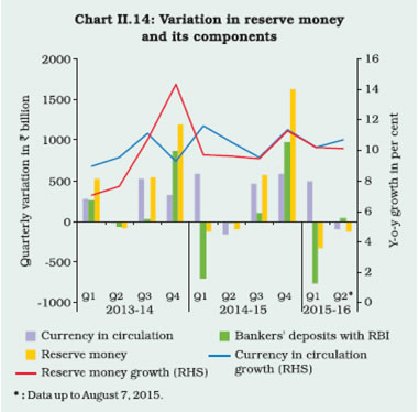
II.3.2 During 2014-15, reserve money expanded
by 11.3 per cent, down from 14.4 per cent a year
ago. On the components side, currency in
circulation, constituting around 75 per cent of
reserve money, increased by 11.3 per cent. The
pick-up in currency demand from 9.2 per cent a
year ago reflected the interaction of several factors
-election-induced demand for currency and
increased food subsidy (Chart II.14). On the other
hand, growth of bankers’ deposits with the Reserve
Bank slowed to 8.3 per cent, mainly reflecting the deceleration in deposit growth. The maintenance
of reserves evened out across 2014-15 following
the introduction of minimum daily CRR balances of
95 per cent since September 2013. Average daily
excess reserve holdings by the banking sector
declined from around 3 per cent in 2013-14 to 2
per cent in 2014-15, which indicated some
efficiency gains under the new liquidity management
framework introduced in September 2014. Variable
rate auctions have induced some discipline in the
banking system in planning liquidity. A system level
liquidity flux appears to have eased with assurance
on availability of liquidity as needed.
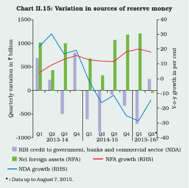
 II.3.3 On the sources side, there was a change
in the composition of reserve money in 2014-15 in
terms of net domestic assets (NDA) and net foreign
assets (NFA). With the emergence of India as a
preferred destination for foreign capital, the Reserve
Bank’s foreign exchange operations to mitigate
undue volatility in the foreign exchange market
resulted in a large increase in NFA, injecting around
₹3.2 trillion primary liquidity (reserve money) into
the financial system. Concomitantly, NDA (adjusted
for net non-monetary liabilities) declined by around
₹1.9 trillion to partially sterilise the impact of the Reserve Bank’s forex market operations on reserve
money expansion.
II.3.4 Global financial markets have been roiled
by turbulence associated with divergence in
monetary policy stances in the G3 economies.
During 2014-15, significant shifts in monetary policy
settings were also observed among emerging
economies to manage the effects of G3 monetary
policies on their financial systems transmitted
through capital flows and asset prices as also to
deal with domestic fragilities which restrained growth and made them vulnerable to financial
shocks. Cross-border externalities associated with
the conduct of unconventional monetary policies in
advanced and emerging economies alike occupied
centre-stage in 2014-15 (Box II.3).
Box II.3
Spillovers and Spillbacks
‘Spillovers’ have come to be commonly employed in the
post-unconventional monetary policy (UMP) literature to
refer to the beneficial or damaging effects that a country’s
economic policies can have on other nations. In the more
recent period, the focus has largely been on negative
externalities associated with the Fed’s quantitative easing
(QE) and its widely anticipated normalisation, especially as
the Fed’s forward guidance on it has been data-dependent
and consequently, every incoming data has triggered intense
market reactions on its possible timing. In the event, UMPs
have generated large capital flows to emerging market
economies (EMEs) in an indiscriminate search for yields,
while exit from them has increased the risks of substantial
capital outflows of which the taper tantrum of the summer
of 2013 provided a sinister preview. Empirical evidence
suggests that UMPs have amplified the pro-cyclicality of
capital flows and leverage in EMEs by strengthening the
incentives to engage in maturity transformations, leading to
misalignment with fundamentals with adverse implications
for macroeconomic and financial stability (Fratzscher et al.
2013; Moore et al. 2013). Quite naturally, spillovers from
UMPs have been the subject of acrimonious disharmony
(Taylor 2013). Given the heterogeneity in the structural
characteristics of EMEs, it is important to nuance these
findings and qualify them with country-specific experiences.
For India, an analysis of the impact of spillovers from the
Fed’s QEs using a combination of methodologies, such as
the event study framework, generalised method of moments
(GMM) and vector auto-regressions (VARs) shows that
the largest favourable impact came from QE1 that pushed
capital flows into India, helping finance a widening current
account deficit. QE2, unlike QE1, was associated with
capital outflows from India. These spillovers were transmitted mainly through the portfolio rebalancing channel, followed
by the liquidity channel (Patra et al. 2014).
‘Spillbacks’ are a new entrant in this proliferating body of
work, essentially the boomerang effects from recipient
countries in a vicious loop that in a globally inter-dependent
world adversely affect the source country that caused the
spillovers in the first place. The larger global role played by
EMEs implies that spillbacks from fluctuations in their growth
as a result of shocks in advanced economies can be nontrivial.
VAR specifications suggest that about 50 per cent
of the fluctuations in outputs in advanced economies spill
over onto EMEs of which one-third spill back to advanced
economies (IMF 2014) (Table 1).
| Table 1: Estimated spillovers and spillbacks (per cent) |
| |
US |
Euro Area |
Japan |
UK |
Average |
| 1 |
2 |
3 |
4 |
5 |
6 |
| EM Spillover |
58.3* |
59.2* |
25.4* |
56.3* |
52.8 |
| EM Spillback |
12.4 |
29.8* |
12.7* |
7.2 |
17.4 |
| EM Spillback/ EM Spillover |
21.3 |
50.4 |
51.1 |
12.8 |
34.4 |
Source: IMF staff calculations.
*: Significant at the 10 per cent level. Estimates of spillovers and
spillbacks from a 1 percentage point increase in growth in advanced
economies (eight quarters after impact). |
Spillback effects are more pronounced for Japan and the
euro area, and less for the United States and the United
Kingdom due to stronger trade linkages (Trade openness
for the US and the UK is relatively far less).
Overall, spillback effects appear to be modest but could
be larger in periods of stress, which in turn might have an adverse impact on the setting of monetary policy. Careful
calibration and clear communication, with cooperation
among policymakers could help in managing spillbacks and
spillovers.
References:
Fratzscher, Marcel, Marco Lo Duca and Roland Straub
(2013), ‘On the International Spillovers of US Quantitative
Easing’, Working Paper Series No. 1557, June.
International Monetary Fund (2014), Spillover Report 2014.
Moore J., S. Nam, M. Suh and A. Tepper (2013),‘Estimating the Impacts of US LSAP’s on Emerging Market Economies’
Local Currency Bond Markets’, Staff Report No. 595,
Federal Reserve Bank of New York.
Patra, M.D., J.K. Khundrakpam, S. Gangadaran, Rajesh
Kavediya and Jessica Anthony (2014), ‘Responding to QE
Taper from the Receiving End’, mimeo, RBI.
Taylor John B. (2013),‘International Monetary Policy
Coordination: Past, Present and Future’, Paper prepared
for presentation at the 12th BIS Annual Conference on
‘Navigating the Great Recession: What Role for Monetary
Policy’, Lucerne, Switzerland, June 21.
II.3.5 In response to these global factors affecting
domestic liquidity conditions, the Reserve Bank
endeavoured to contain the expansionary effects
in keeping with its commitment to the glide path of
disinflation. The Reserve Bank, therefore,
appropriately calibrated repo auctions and open market operation (OMO) sales, both outright and
on the Negotiated Dealing System-Order Matching
(NDS-OM) platform to contract NDA and offset the
large increase in NFA (Chart II.15).
 II.3.6 Quarterly movements in reserve money in
2014-15 evolved in line with changing drivers of
liquidity and resulting composition shifts in the
Reserve Bank’s balance sheet. On the components
side, except for the seasonal decline in Q2, currency
in circulation increased throughout the year. On the
sources side, the increase in NFA was largely offset
by a decline in NDA in the H1 of 2014-15. In Q4,
however, end year balance sheet adjustments and advance tax payments tightened liquidity conditions,
warranting injection of primary liquidity that
remained largely unsterilised. Consequently,
reserve money growth increased in the last quarter
of 2014-15.
II.3.7 There was also a change in the composition
of NDA during 2014-15 which was in accordance
with modifications in the Reserve Bank’s accounting
policies as recommended by the Technical
Committee formed to review the format of the
balance sheet and the profit and loss account of
the Reserve Bank (Chairman: Shri Y.H. Malegam).
Specifically, net repo operations are now being
recorded under the Reserve Bank’s credit to banks
and commercial sector rather than in its credit to
general government as was done earlier. These
accounting changes are reflected in a decline in
the Reserve Bank’s net credit to the government
and the commensurate increase in its net claim on
banks in 2014-15, though the absolute size of NDA
remains unaffected.
II.3.8 Movements in reserve money influence the
broader measures of money supply through the
money multiplier. In terms of magnitude, the money
multiplier stood at 5.5 in March 2015, unchanged
from its level a year ago. Both the cash deposit ratio
and the cash reserve ratio remained unchanged over
the year, imparting stability to the money multiplier.
Money Supply
II.3.9 The money supply growth slowed down in
2014-15 (Table II.8), mainly reflecting easing
inflation which lowered the demand for money. The
slowdown in money supply in general, and in
aggregate deposits in particular, vis-à-vis 2013-14
has to be seen in the context of the base effect
caused by the swap facility for FCNR(B) deposits
operated by the Reserve Bank during September-
November 2013 which led to high mobilisation of
these deposits in 2013-14. Money supply net of
FCNR(B) deposits was marginally lower in 2014-15
than in the preceding year. However, money supply
improved in the second half of the year (March 2015
over September 2014) in line with the growth in
credit. In tandem, the year-on-year growth in the
liquidity aggregate L1 [sum of the new monetary
aggregate (NM3) and postal deposits] remained
marginally lower than a year ago.
| Table II.8: Monetary Aggregates |
| Item |
Outstanding as on (₹ billion) |
Year-on-year growth rate (in per cent) |
Growth rate (in per cent) |
| March 31,
2015 |
August 7,
2015 |
2013-14 |
2014-15 |
2015-16
(as on
August 7) |
FY 15:
H1 |
FY 15:
H2 |
FY16:
H1 |
| 1 |
2 |
3 |
4 |
5 |
6 |
7 |
8 |
9 |
| I. Reserve Money |
19,285 |
18,815 |
14.4 |
11.3 |
10.1 |
-1.4 |
12.9 |
-2.4 |
| II. Broad Money (M3) |
105,455 |
109,830 |
13.4 |
10.8 |
10.9 |
4.4 |
6.2 |
4.1 |
| III. Liquidity Aggregate (L1) |
106,759 |
110,722# |
11.2 |
10.7 |
11.6# |
4.0 |
6.5 |
3.7# |
| IV. Major Components of M3 |
|
|
|
|
|
|
|
|
| IV.1. Currency with the Public |
13,863 |
14,251 |
9.2 |
11.3 |
9.5 |
3.4 |
7.6 |
2.8 |
| IV.2. Aggregate Deposits |
91,446 |
95,567 |
14.1 |
10.6 |
11.2 |
4.4 |
5.9 |
4.5 |
| V. Major Sources of Money Stock (M3) |
|
|
|
|
|
|
|
|
| V.1. Net Bank Credit to Government |
30,062 |
33,781 |
12.4 |
-1.3 |
10.6 |
-0.5 |
-0.8 |
12.4 |
| V.2. Bank Credit to Commercial Sector |
70,396 |
71,627 |
13.7 |
9.2 |
9.0 |
2.3 |
6.8 |
1.7 |
| V.3. Net Foreign Exchange Assets of the Banking Sector |
22,506 |
23,664 |
17.6 |
17.0 |
16.0 |
3.9 |
12.6 |
5.1 |
| M3 Net of FCNR(B) |
102,782 |
107,009 |
11.5 |
11.0 |
11.1 |
4.4 |
6.3 |
4.1 |
| M3 Multiplier |
5.5 |
5.8 |
|
|
|
|
|
|
| M3 Velocity |
1.25 |
- |
|
|
|
|
|
|
-: Not available;
#: Data pertain to July 2015.
Note: 1. Data are provisional.
2. FY 15: H1: Growth rate of September 2014 over March 2014,
FY 15: H2: Growth rate of March 2015 over September 2014, and
FY 16: H1: Growth rate of August 7, 2015 over March 31, 2015. |
II.3.10 Growth in aggregate deposits, which forms
a major component of money supply, has generally
been declining over the years in line with a decrease
in the saving rate of the economy. In addition,
slowdown in credit growth led to lower deposit
mobilisation by banks. The growth in aggregate
deposits decelerated to 10.6 per cent in 2014-15
from 14.1 per cent a year ago. On the sources side,
a decline in banks’ credit growth to the commercial
sector was one of the key drivers. Another major
constituent from the sources side, that is, net bank
credit to the government declined during the year
mainly due to reduction in the Reserve Bank’s
holding of government securities (G-secs).
Commercial banks, on the other hand, stepped up
their investment in G-secs in view of credit
deceleration during the year.
II.3.11 The velocity of money (Chart II.16), which
declined over the past six decades hovered around 1.25, indicating stability of the financial system in
the post-crisis years. Another commonly referred
indicator of financial deepening - M3 to GDP
ratio - which is a reciprocal of velocity, stood at
around 80.
CREDIT
II.3.12 Non-food credit growth decelerated
sharply in 2014-15 to 9.3 per cent (y-o-y), with
incremental non-food credit declining to ₹5.5
trillion from ₹7.3 trillion in the previous year. A
host of factors weighed down on credit off-take,
including lower corporate sales, softening of
inflation rate, risk aversion by banks due to rise
in non-performing loans, and procedural delays
in debt recovery (Box II.4). Further, with the
availability of alternative sources, both domestic and foreign, corporates switched some of the
demand for financing to non-bank sources. Sale
of significantly larger amount of non-performing
loans (₹317 billion) by banks to asset
reconstruction companies (ARCs) during 2014-
15 also contributed to a deceleration in bank
credit. Food credit also registered a decline of
4.1 per cent during the year, despite some pickup
in procurement, as a result of enhanced food subsidies which increased by 28.1 per cent in
2014-15.
Box II.4
Factors Underlying Recent Credit Slowdown: An Empirical Exploration
Credit plays an important role in economic development,
particularly in a bank-based financial system. Countries which
experienced high growth since 2000 also witnessed a surge
in private credit (Claessens et al. 2011). An empirical analysis
also suggests that credit growth is positively influenced by
deposit growth, GDP growth, easy global liquidity conditions
and exchange rate depreciation, whereas inflation dampens
real credit growth (Guo and Stepanyan 2011). In India’s bankbased
financial system, credit plays an important role in the
overall growth dynamics.
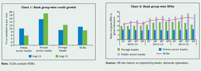
Asset quality concerns resulting in risk aversion are
considered to be one of the major factors underlying the
current slowdown in credit. Public sector banks, which
recorded higher NPA ratios, experienced a sharp decline in
credit growth. On the other hand, private sector banks with
lower NPA ratios, posted higher credit growth (Chart 1 and
2). At the aggregate level, the NPA ratio and credit growth
exhibited a statistically significant negative correlation of 0.8,
based on quarterly data since 2010-11.
 Applying the methodology of Guo and Stepanyan (2011) to
Indian quarterly data from June 1997 to September 2014,
non-food credit was found to be influenced by lagged real
GDP growth in a positive and statistically significant manner.
The cost of credit proxied by the overnight call rate, as
expected, had a negative impact on credit growth. The impact
of the interest rate was found to be strong up to two lags,
reflecting transmission lags. In line with the theory, the
coefficient of gross fiscal deficit (GFD) of the Centre had a
negative sign, indicating crowding out effects of fiscal deficit
in market for bank credit. Finally, the change in outstanding
commercial papers (CPs), a proxy for an alternative source
of funds, had a negative and significant coefficient.
Adjusted R2=0.30; *: Significant at 5 per cent;
NPAs were not included in the regression as the series had multiple
structural breaks.
Note: 1. BC=q-o-q seasonally adjusted growth in bank credit;
WCMR=quarterly weighted average call rate; GDP= q-o-q seasonally
adjusted growth in GDP (base: 2004-05); GFD: quarterly GFD (Centre)
as per cent of GDP at current market price; CP_out: q-o-q seasonally
adjusted growth in CP outstanding.
2. The results were subjected to standard robustness checks.
Thus economic activity, cost of credit, the fiscal position and
competitive alternative funding sources turned out to be major
factors affecting credit behaviour in India.
References:
Claessens, S., M. A. Koseand M.E. Terrones (2011), ‘How Do
Business and Financial Cycles Interact?’, IMF Working Paper,
No. WP/11/88.
Guo K. and V. Stepanyan (2011), ‘Determinants of Bank Credit
in Emerging Market Economies’, IMF Working Paper
WP/11/51.
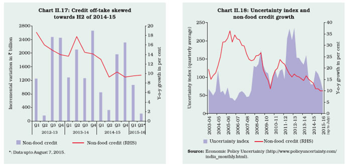
II.3.13 With the deceleration in non-food credit
growth on a year-on-year basis, nearly 80 per cent
of the incremental credit off-take during 2014-15
took place in the second half of the year, reflecting
the improving economic environment (Charts II.17
and II.18). Non-food credit growth increased to 7.1 per cent in H2 of 2014-15 from 2.0 per cent in H1,
representing an improvement of 5 percentage
points in H2 compared with 0.6 percentage point
increase a year ago.
 II.3.14 In order to create more space for banks to
expand credit to the productive sectors of the
economy, the statutory liquidity ratio (SLR) was
reduced in three stages from 23 per cent to 21.5
per cent of net demand and time liabilities (NDTL)
during 2014-15. However, banks continued to
maintain SLR investments around 28 per cent of
NDTL, the buffer providing access to collateralised
borrowings from the wholesale funding market and
the Reserve Bank. Maintaining excess SLR
securities also helped banks to weather the impact
of the current slow phase of the economic cycle on
their balance sheets and earnings.
II.3.15 Data on sectoral deployment of credit, which
constitutes about 95 per cent of total bank credit
by SCBs, indicate that deceleration in credit off-take in 2014-15 was more pronounced with respect to
the industry and services sectors, which together
constituted about 68 per cent of total non-food
credit. Credit growth in the services sector was
weighed down by its major components: trade and
non-banking financial companies (NBFCs) that
accounted for nearly 48 per cent of the total credit
to the services sector. In the industrial sector,
growth slowed down across sectors, particularly for
infrastructure, basic metals and food processing.
The sectors which witnessed lower incidence of
NPAs such as personal loans saw higher growth
during the year.
II.3.16 Infrastructure accounts for nearly one-third
of the credit to the industrial sector. Its main
components are power and roads, constituting 60
and 18 per cent of the total infrastructure credit
respectively. While deceleration in credit to the
power sector was modest, the slowdown was sharp
with respect to roads in 2014-15 (Table II.9).
| Table II.9: Trends in Credit Deployment to Select Sectors |
| (Variation in per cent) |
| |
Outstanding at
20-Mar-2015
(₹ billion) |
2013-14 |
2014-15 |
2015-16 |
| H1 |
H2 |
Year |
H1 |
H2 |
Year |
H1 |
| 1 |
2 |
3 |
4 |
5 |
6 |
7 |
8 |
9 |
| Non-food Credit (1 to 4) |
60,030 |
6.8 |
6.3 |
13.6 |
2.2 |
6.2 |
8.6 |
1.1 |
| 1. Agriculture & Allied Activities |
7,659 |
3.4 |
9.2 |
12.9 |
8.8 |
5.7 |
15.0 |
3.8 |
| 2. Industry |
26,576 |
6.3 |
6.1 |
12.8 |
-0.1 |
5.7 |
5.6 |
-1.0 |
| Of which: |
9,245 |
8.8 |
5.3 |
14.6 |
4.3 |
6.0 |
10.5 |
1.0 |
| (i) Infrastructure |
|
|
|
|
|
|
|
|
| Of which: (a) Power |
5,576 |
10.7 |
5.8 |
17.1 |
6.6 |
7.5 |
14.5 |
2.8 |
| (b) Telecommunications |
919 |
-0.6 |
1.1 |
0.5 |
-3.6 |
8.0 |
4.2 |
-2.9 |
| (c) Roads |
1,687 |
9.2 |
10.1 |
20.2 |
3.5 |
3.3 |
6.9 |
-0.7 |
| (ii) Basic Metal & Metal Product |
3,854 |
7.2 |
7.1 |
14.9 |
-0.4 |
7.2 |
6.8 |
-0.6 |
| (iii) Food Processing |
1,715 |
3.5 |
20.4 |
24.6 |
-2.6 |
20.4 |
17.3 |
-6.2 |
| 3. Services |
14,131 |
9.0 |
6.5 |
16.1 |
-1.2 |
6.9 |
5.7 |
1.4 |
| 4. Personal Loans |
11,663 |
7.5 |
4.6 |
12.5 |
8.0 |
6.9 |
15.5 |
4.0 |
| Note: Latest available data for H1 of 2015-16 are up to June 2015. |
II.3.17 During 2015-16 so far (up to August 7),
credit off-take seems to be picking up reflecting
an improving economic and policy environment,
though it is too early for a conclusive evidence.
Incremental non-food credit stood around
₹1,282 billion as against ₹963 billion during the
corresponding period last year. Data on sectoral
deployment (up to June 2015) reveal a
significant pick-up in services mainly supported
by trade and professional services, while
industry registered a decline. Within industry,
although credit to infrastructure shows signs of
pick-up, that to roads continues to be weak
(Chart II.19).
Non-bank funding
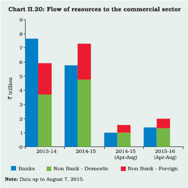
II.3.18 Slowdown in credit growth dragged down
the overall flow of financial resources to the
commercial sector in 2014-15, despite higher
recourse to non-bank sources of funds (Chart
II.20). Amongst the non-bank domestic sources, net issuance of CPs witnessed a four-fold
increase during the year, mainly attributable to
competitive pricing vis-á-vis banks’ lending
rates. Further, FDI inflows remained strong and
accounted for a major chunk of the non-bank
foreign resources to the commercial sector.
Reliance on non-bank sources continues during
2015-16 so far (up to August 7) amidst
comfortable liquidity conditions and competitive
rates.
 II.3.19 Regime shifts in the conduct of monetary
policy shaped monetary and credit conditions in
2014-15. Money supply and other key monetary
aggregates decelerated in line with underlying
macroeconomic activity. Overall, credit growth was
subdued during 2014-15 owing to various factors,
such as risk aversion by banks due to rising NPAs
and alternative and cheaper sources of non-bank
funding, though there was some evidence that a
turnaround in the second half of the year might have
set in.
II.4 FINANCIAL MARKETS
Global Financial Markets
II.4.1 International financial markets remained
generally upbeat during 2014-15, lifted by
expectations of a relaxed approach of the US
Federal Reserve to monetary policy normalisation,
quantitative easing by the European Central Bank
(ECB) and the Bank of Japan (BoJ) and decline in
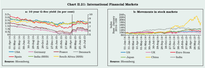
crude oil prices. Government bond yields for most
of the countries were historically low with some
European countries even experiencing negative
yields (Chart II.21a). A number of stock markets
also reached historical highs during 2014-15 as
fears about US monetary policy rates lifting off
receded and the ECB and the BoJ enhanced their
asset purchase programmes. However, markets
experienced some volatility in mid-October 2014
on account of uncertainty on the global recovery,
a slew of weak data from the US and the euro area
and continuing geo-political tensions in the Middle
East. Again in the second half of December 2014,
markets were affected by the Ukrainian crisis
followed by the Russian currency crisis and large
exchange rate depreciation in Venezuela and
Argentina (Chart II.21b).
II.4.2 The US dollar index, which measures the
dollar’s movement against other major currencies,
strengthened by 23 per cent from 80.1 at end-March 2014 to 98.4 at end-March 2015. While it
strengthened primarily on account of a robust US
economic recovery, weak economic recovery in the
euro zone and Japan during the year resulted in
the euro and the Japanese yen depreciating against
the US dollar. In January 2015, as ECB prepared
to announce quantitative easing, the Swiss National
Bank (SNB) abandoned its cap on the Swiss franc/
euro exchange rate which led to heightened
exchange rate volatility. During Q4 of 2014-15, a
number of emerging markets and developing
economies (EMDEs) reduced their policy rates to
support economic growth. Interventions in foreign
exchange markets to address depreciating
pressures also increased.
II.4.3 In May 2015, markets were surprised by the
global bond sell-off that started in Germany as the
10-year German Bund yield increased to intra-day
high of 0.77 per cent on May 7 from 0.05 per cent
on April 17, 2015. Concerns over Greek debt,
sustained increase in crude oil prices and profit
booking quickly transmitted to US treasury bills as
well as emerging market economies.
II.4.4 During June 2015, movements in
international financial markets were abuzz with
uncertainty relating to the outcome of Greek debt
negotiations and meltdown in the Chinese stock
market. However, in July financial markets received support from the announcement of the bailout deal
between Greece and the euro zone members and
signing of the nuclear deal between Iran and major
world powers. In August, the global financial
markets were shaken by China’s decision to
devalue its currency by around 2 per cent.
Indian Financial Markets
II.4.5 Both domestic and global cues were at play
in buoying Indian financial markets during 2014-15.
Equity markets reached all-time highs during the
year. Money markets were stable and liquid with
call money rate evolving tightly around the policy
repo rate. Yields on government securities (G-secs)
declined gradually and activity in the corporate bond
market registered an increase mainly due to
primary issuances.
Money Market
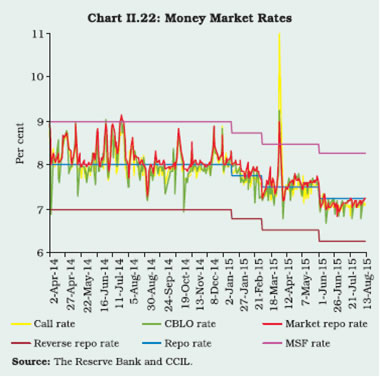
II.4.6 Overnight call money rates remained closely
aligned to the policy repo rate, with active liquidity
management operations under the revised liquidity
management framework, except adjustment for the
year-end window dressing. Money market rates
declined in Q4 in sync with cuts in the policy rate
(Chart II.22). With deposit growth generally
remaining above credit growth during the year,
structural liquidity conditions remained comfortable.
During 2015-16 so far, call money rates have
remained aligned to the policy repo rate with money
market rates declining after the cut in policy rate on
June 2, 2015.
 II.4.7 The spread of the daily weighted average
call rate (excluding Saturdays) over the policy rate
narrowed down significantly during 2014-15 from
30 basis points (bps) to 18 bps after the adoption
of the revised liquidity management framework in
September 2014. The spread further narrowed
down to 16 bps during 2015-16 (upto August 14).
The spread of collateralised rates (CBLO and
market repo) also narrowed down during this period, indicating synchronised movement among overnight
money market rates. The collateralised segment
continued to attract a major portion of the turnover
in the overnight market, with the uncollateralised
(call money) segment registering relatively thin
volumes, rendering it susceptible to bouts of
volatility. A large part of the assured liquidity support
under the Reserve Bank’s liquidity adjustment
facility (LAF) is being offered through variable rate
term repos with one of its main objectives being
development of the term money market.
Notwithstanding these initiatives, the turnover in the
term money market has remained muted.
Issuance of CDs and CPs
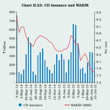
II.4.8 The average fortnightly issuance of
certificates of deposits (CDs) decreased to ₹297
billion during 2014-15 from ₹306 billion during the
previous year (Chart II.23). The easing of liquidity
conditions, coupled with a reduction in the policy
rate and relatively lower issuances of CDs by banks
on the back of subdued credit off-take, led to a
decrease in the weighted average effective interest
rate (WAEIR) on CDs from 9.74 per cent at end-
March 2014 to 8.58 per cent at end-March 2015. The easing trend has continued during 2015-16 so
far with WAEIR declining further to 7.79 per cent
by July 10, 2015.
 II.4.9 The average fortnightly issuance of
commercial papers (CPs) increased by 58 per cent
to ₹479 billion during 2014-15, reflecting substitution
of short-term bank credit by market based funding
on account of the cost effectiveness of CPs for
raising funds on the back of significant easing of
yields on corporate bonds (Chart II.24). Consequently,
the outstanding amount of CPs stood higher at
₹1,933 billion at end-March 2015 as compared to
₹1,066 billion at end-March 2014. The weighted
average discount rate (WADR) for CPs decreased
to 9.26 per cent at end-March 2015 from 9.92 per
cent at end-March 2014, reflecting easing of liquidity
conditions during the year and overall downward
movement in the interest rate cycle. The declining
trend has continued during 2015-16 so far with
WADR standing at 7.97 per cent at end-July 2015.
Yields in the G-Secs Market
II.4.10 G-secs yields generally softened through
2014-15, reflecting easing of US treasury yields, active buying interest by foreign portfolio investors
(FPIs), sharp decline in inflation, improvement in
the fiscal situation, positive sentiment after the
general elections, steep decline in international oil
prices and cuts in policy rate by the Reserve Bank.
Some uptick in yields occurred in June and July
2014 due to geo-political tensions in the Middle
East as also the announcement of higher net
market borrowing in the Union Budget for 2014-15.
Yields spiked again in the second half of December
2014 on account of geo-political tensions and the
Russian currency crisis. However, the yields
softened in Q4 following increased buying by FPIs.
Sustained buying interest in government debt by
FPIs was discernible as their limit remained almost
fully utilised, notwithstanding certain conditions
such as debarring FPIs from investing in treasury
bills and permitting incremental investment only in
G-secs with minimum residual maturity of three
years. Notably, the G-secs market weathered the
impact of a complete exit from the assets purchase
programme by the Federal Reserve in October
2014 with the yields continuing to exhibit a softening
bias on the back of buoyant investor sentiment
(Chart II.25).
 II.4.11 Bearish sentiment took hold in the G-secs
market in February 2015 for a variety of reasons,
including, but not limited to, a broadly unchanged
size of the government market borrowing programme
for 2015-16 and rescheduling of the fiscal
consolidation plan by a year as announced in the
Union Budget for 2015-16. However, the follow-up
policy rate cut of 25 bps each on January 15, 2015
and March 4, 2015, coupled with a sharp fall in US
treasury yields, buoyed the market sentiment and
led to softening of the 10-year G-Sec yield. The
improvement in sentiment was short-lived after a
status quo on the policy rate was announced in the
bi-monthly monetary policy on April 7, 2015. More
pertinently, taking cues from hardening of long-term
bond yields in most of the advanced economies on
the back of improved growth and inflation outlook,
and hardening oil prices, the 10-year yield on Indian
G-secs rose during the first half of May 2015,
touching a high of 8.09 per cent on May 11, 2015.
The yield has, however, softened thereafter with
the introduction of a new 10-year benchmark
security, cut in policy rate and significant decline in
inflation. The 10-year yield stood at 7.75 per cent
on August 14, 2015. The average volume generally varied inversely with the movement in 10-year
G-sec yield barring the period from October to
November 2014 (Chart II.26). The G-secs turnover
ratio moved up to 1.95 per cent in 2014-15 from
1.87 per cent in the previous year.
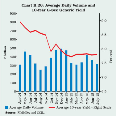 FPI Flows into India
II.4.12 FPIs in the equity and debt markets in India
revived during 2014-15. While FPI inflows to the
debt market turned positive at ₹1.6 trillion facilitated
by an increase in the FPI sub-limit by US$ 5 billion
within the overall limit of US$ 30 billion, FPI
investments in equity markets were also higher than
they were in 2013-14 (Chart II.27). Currently, FPI
investors are permitted to invest only in bonds with
the minimum residual maturity of three years so as
to encourage investments in long term securities
and to contain interest rate volatility at the shorter
end. The effective FPI limit was increased by
allowing FPIs to invest coupons from G-secs,
outside the overall limit, with effect from February
5, 2015. During 2015-16 so far (up to August 13,
2015), FPI flows in the debt and equity markets
have been subdued at ₹(-)43.2 billion and ₹47.4
billion, respectively, following the global bond sell off triggered in the European bond markets on May
7, 2015, concerns over weak quarterly earnings
reported for Q4, as also over the minimum alternate
tax (MAT) and increased uncertainty in the global
financial markets.
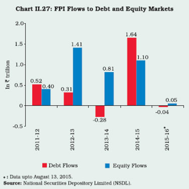 Corporate Bond Market
II.4.13 During 2014-15, turnover in the corporate
bond market increased by 12 per cent to ₹10,913
billion (Chart II.28a). On the other hand, the yield
spread of 5-year AAA rated corporate bonds over
G-secs of corresponding maturity declined until
mid-November 2014 following the crash in global
crude oil prices, stability in the exchange market and Moody’s outlook upgrade. Subsequently,
however, frictional liquidity pressure on account of
advance tax payments and concerns over the rise
in the current account deficit for Q2 of 2014 led to
a widening of the spreads until mid-January 2015.
Following the cuts in the policy repo rate and
improved liquidity conditions, yield spreads declined
in Q4 of 2014-15 (Chart II.28b). During 2015-16 so
far, the yield spread remained range bound,
indicating easy liquidity conditions.
Secondary Equity Market
II.4.14 The equity market witnessed heightened
activity in 2014-15, scaling new highs on January
29, 2015 (Chart II.29a). During the year, the BSE
Sensex rose by 25 per cent on top of the uptick of
19 per cent in 2013-14. Equity market sentiment
was supported by political stability, sustained FPI
flows, lower international crude oil prices and
softening of the policy rate.
II.4.15 The equity market was also supported by
global liquidity conditions and the search for yield
aided by the US Federal Reserve’s commitment to
low interest rates, ultra-accommodative monetary
policies pursued by the ECB, the BoJ and the
People’s Bank of China. In US dollar terms, the
Sensex rose by 20 per cent, turning out to be one
of the best performing markets in the world (Chart
II.29b). The domestic equity market also witnessed
lower volatility in 2014-15 as compared to equity
markets abroad.
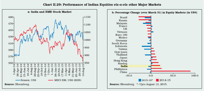 II.4.16 During 2015-16, equity markets had a
subdued start on account of FPIs’ concern over
MAT, weak Q4 corporate earnings and forecast of
a below normal monsoon. However, benchmark
indices recovered after realisation of above normal
rainfall in June. Domestic markets also received
support from positive developments relating to
Greece and the Iran nuclear deal. In August 2015,
the stock markets remained range bound guided,
among others, by mixed earnings for Q1 of 2015-16
and global developments such as China’s currency
devaluation.
Primary Equity Market
II.4.17 During 2014-15, resource mobilisation
through equity issues, including qualified
institutional placement (QIP) rose significantly by
44 per cent (Table II.10). There were signs of
renewed interest in initial public offerings (IPOs)
with an increase in the number of companies filing
draft red herring prospectuses (DRHPs) with the
Securities and Exchange Board of India (SEBI) to
raise resources in 2015-16. Going forward, positive
sentiment in the secondary market, if sustained,
will help raise larger resources through the primary
market.
| Table II.10: Primary Capital Market Mobilisation |
| (₹ billion) |
| Category |
2011-12 |
2012-13 |
2013-14 |
2014-15 (P) |
| 1 |
2 |
3 |
4 |
5 |
| a. Public Issues (i)+(ii) |
460.9 |
219.2 |
510.8 |
127.5 |
| (i) Public Issues (Equity) |
104.8 |
49.4 |
87.0 |
30.4 |
| Of which |
|
|
|
|
| IPOs |
59.0 |
49.4 |
12.4 |
30.4 |
| FPOs |
45.8 |
0.0 |
74.6 |
0.0 |
| (ii) Public Issues (Debt) |
356.1 |
169.8 |
423.8 |
97.1 |
| b. Rights Issues |
23.7 |
89.4 |
45.8 |
67.5 |
| Total Equity Issues (i+b) |
128.6 |
138.8 |
132.7 |
97.9 |
| c. Euro Issues (ADR/GDR) |
27.1 |
10.4 |
1.2 |
95.9 |
| d. Mutual Fund Mobilisation (net) |
-220.2 |
765.4 |
537.8 |
1032.9 |
| 1. Private Sector |
-154.5 |
637.9 |
488.4 |
1037.0 |
| 2. Public Sector |
-65.8 |
127.5 |
49.4 |
-4.1 |
| e. Private placements in the corporate debt market |
2612.8 |
3614.6 |
2760.5 |
4041.4 |
| f. QIP |
21.6 |
160.0 |
136.6 |
291.0 |
P: Provisional;
IPOs: Initial public offerings;
FPOs: Follow on public offers;
ADR: American depository receipts;
GDR: Global depository receipts;
QIP: Qualified institutional placement.
Source: SEBI and Prime database. |
Private Placement of Corporate Bonds
II.4.18 Mobilisation through private placement of
corporate bonds at ₹4,041 billion was significantly
higher by 46 per cent during 2014-15, while public
issues of non-convertible debentures at ₹97 billion
were much lower. Mobilisation through public issues
of bonds is set to witness a revival in 2015-16 with
the Union Budget 2015-16 proposing to raise
resources through tax-free bonds for funding
infrastructure.
II.4.19 The Central Government has budgeted a
receipt of ₹695 billion through disinvestment in
2015-16, of which ₹285 billion is expected to be
mobilised through strategic disinvestments.
Measures, such as the introduction of e-IPO norms
and allowing firms to launch real estate investment
trusts (REITs) and infrastructure investment trusts
(InvITs) as also the government’s disinvestment
measures are expected to provide an impetus to
the capital markets going forward.
House Price Index (HPI)
II.4.20 Quarterly growth (y-o-y) in HPI went below
16 per cent in Q1 of 2013-14 and further down in Q3 mainly due to subdued demand. However, it
moved up in the first three quarters of 2014-15,
suggesting a moderate pick up in house price
growth, particularly in cities like Delhi and Kolkata
(Chart II.30). The demand for residential properties
has slowed down in recent times and unsold stock
of residential homes has increased considerably
at the same time. Genuine home buyers moved
away from the housing market due to higher prices
and investors stayed away due to the weakening
state of the economy. As the economic growth has
started to take-off, the overall buyer sentiment is
expected to rise. Presumably, developers are
counting on this to happen and hence holding the
price.
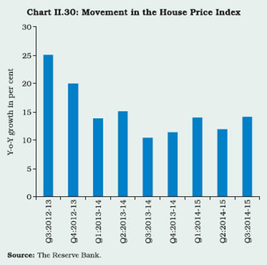 II.4.21 Financial markets in India performed well
during 2014-15. Money market rates closely
followed the policy repo rate; and in the backdrop
of sluggish credit growth and relatively comfortable
structural liquidity, coupled with policy rate easing
by the Reserve Bank, the rates on CPs and CDs declined during the year. G-secs yields generally
softened in 2014-15 in line with a decline in inflation
and continued buying interests by FPIs. Equity
markets, primary as well as secondary, fared better
than in the previous year.
II.5 GOVERNMENT FINANCES
II.5.1 Public finances have been gradually improving
at the level of both the Centre and the states. The
impetus for rectitude has mainly emanated from a
re-commitment to calibrated paths of fiscal
consolidation in the post-global crisis period. Initially
quantity-driven, these efforts have been guided by
the imperative to stabilise fiscal consolidation on
the chosen trajectories and then to re-order
expenditure priorities from subsidies to investment,
to raise tax buoyancy, to rationalise nondevelopmental
spending and leakages and to
contain public debt at sustainable levels for all layers
of the government. With annual budgetary targets
for the gross fiscal deficit (GFD) met since 2012-13,
attention has increasingly turned to the quality of
fiscal consolidation. Key deficit indicators of the
Central Government were lower in 2014-15, as per
the provisional accounts (PA), than a year ago. GFD
was lower than the budgetary target, both in
absolute terms and as percentage of GDP.
Centre: Receipts and Expenditure
II.5.2 In 2014-15 (provisional accounts), non-debt
receipts were sluggish reflecting tepid domestic
activity. While gross tax collection suffered a
shortfall of 8.8 per cent from the budget estimates (BE), net tax inflows turned out to be 7.7 per cent
lower than BE, mainly on account of subdued
indirect tax receipts. Non-tax revenue was also
lower than BE due to lower collections from general,
economic, fiscal and social services. Non-debt
capital receipts were significantly lower than the
budgetary target, reflecting a large shortfall in
disinvestment proceeds.
II.5.3 The shortfall in non-debt receipts warranted
a sharp cutback in plan expenditure by more than
20 per cent, both on the revenue and capital
accounts, in order to meet deficit targets. A marginal
reduction in non-plan expenditure over BE was also
effected through reduction in capital expenditure
and interest payments.
II.5.4 Both overall capital expenditure and capital
outlay were lower than budgeted levels and also
lower than last year’s levels. This has potentially
adverse implications for growth in the medium term.
Recalibration of the Fiscal Consolidation Path in
2015-16
II.5.5 Union Budget 2015-16 has carried forward
the process of fiscal consolidation, with all the key
deficit indicators projected to decline (Table II.11).
The targeted reduction in GFD is proposed to be attained by a compression in revenue expenditure
combined with an increase in non-debt capital
receipts. The goalpost for achieving the GFD-GDP
target of 3.0 per cent under the FRBM Act/Rules
has been shifted by a year to 2017-18 mainly to
accommodate higher public investment to support
growth, and higher devolution to the states following
the recommendations of 14th Finance Commission
as also accounting for uncertainties associated with
the implementation of the Goods and Services Tax
(GST) and the likely burden of the 7th Pay
Commission award.
| Table II.11: Fiscal Performance of the Central Government |
| (Per cent of GDP) |
| Variables |
2004-08 (Avg) |
2008-10 (Avg) |
2010-14 (Avg) |
2013-14 |
2014-15(RE) |
2014-15 (PA) |
2015-16 (BE) |
| 1 |
2 |
3 |
4 |
5 |
6 |
7 |
8 |
| Non Debt Receipts |
10.4 |
9.5 |
9.5 |
9.3 |
9.3 |
9.1 |
8.7 |
| Tax revenue |
7.8 |
7.5 |
7.3 |
7.2 |
7.2 |
7.2 |
6.5 |
| Non-tax revenue |
2.1 |
1.8 |
1.8 |
1.8 |
1.7 |
1.6 |
1.6 |
| Non debt capital receipts |
0.4 |
0.3 |
0.4 |
0.4 |
0.3 |
0.3 |
0.6 |
| Total Expenditure |
14.2 |
15.8 |
14.5 |
13.7 |
13.4 |
13.1 |
12.6 |
| Revenue expenditure |
11.9 |
14.1 |
12.7 |
12.1 |
11.9 |
11.6 |
10.9 |
| Capital expenditure |
2.3 |
1.7 |
1.8 |
1.7 |
1.5 |
1.5 |
1.7 |
| Plan expenditure |
4.0 |
4.8 |
4.4 |
4.0 |
3.7 |
3.6 |
3.3 |
| Non-plan expenditure |
10.2 |
11.0 |
10.1 |
9.7 |
9.7 |
9.5 |
9.3 |
| Revenue Deficit |
2.0 |
4.9 |
3.6 |
3.1 |
2.9 |
2.9 |
2.8 |
| Gross Fiscal Deficit |
3.4 |
6.2 |
5.0 |
4.4 |
4.1 |
4.0 |
3.9 |
Note: 1. Avg: Average; RE: Revised Estimates; PA: Provisional Accounts; BE: Budget Estimates.
2. GDP 2014-15 is as per Provisional Estimates of CSO. |
Targets for Indirect Taxes and Disinvestment
Proceeds
II.5.6 With an expected growth of 16.4 per cent in
gross tax revenue, the ratio of gross tax revenue to
GDP is estimated to improve by 0.4 percentage
points to 10.3 per cent in 2015-16. The net tax
revenue accruing to the Centre is, however,
budgeted significantly lower at 6.5 per cent of GDP
– down from 7.2 per cent in 2014-15 (PA) due to
higher devolution to the states following the 14th
Finance Commission award. The implied tax
buoyancy for gross tax revenue is significantly
higher than the realised buoyancy of less than 1 in
the previous two years (Table II.12). Further, the
projected increase of 18.9 per cent in indirect taxes
as against 9.8 per cent realised in 2014-15 (PA)
assumes a buoyancy of about 2 for service tax on the back of a hike in the service tax rate (inclusive
of education cess) by 1.64 per cent, pruning of the
Negative List under service tax and withdrawal of
certain other exemptions to widen the tax base. The
projected buoyancy of 1.73 in the case of excise
duty collections is mainly supported by ad hoc hikes
in excise duty on petrol and diesel in 2014-15,
increase in excise duty on select products, such as
mobile handsets and cigarettes, imposition of
excise duty on hitherto untaxed items like condensed
milk and peanut butter, and a general increase in
excise duty to 12.5 per cent from the prevailing
12.36 per cent. While these measures will facilitate
meeting budgeted targets for indirect tax collections
in 2015-16, it is crucial to adhere to the timeline for
the rollout of GST for a sustainable increase in tax
revenues in the medium term.
| Table II.12: Tax Buoyancy and Growth Rates in Tax Collections* |
| Tax Categories |
Tax Buoyancy |
Growth Rates (Per cent) |
| 2013-14 |
2014-15(PA) |
2015-16 (BE) |
2013-14 |
2014-15(PA) |
2015-16 (BE) |
| 1 |
2 |
3 |
4 |
5 |
6 |
7 |
| Gross Tax Revenue |
0.73 |
0.89 |
1.31 |
9.9 |
9.3 |
16.4 |
| Corporation Tax |
0.79 |
0.82 |
0.78 |
10.8 |
8.7 |
9.7 |
| Income Tax |
1.55 |
0.82 |
1.93 |
21.0 |
8.6 |
24.2 |
| Customs Duty |
0.30 |
0.88 |
0.86 |
4.1 |
9.3 |
10.8 |
| Union Excise Duty |
-0.24 |
1.05 |
1.73 |
-3.2 |
11.1 |
21.6 |
| Service Tax |
1.23 |
0.81 |
1.99 |
16.7 |
8.5 |
24.9 |
| *: Buoyancies are worked out with respect to overall GDP growth rate. |
II.5.7 Non-tax revenue, which includes dividends
from public sector undertakings (PSUs), the
Reserve Bank, PSU banks and spectrum charges,
is budgeted to grow at 12.6 per cent in 2015-16.
Disinvestment proceeds are budgeted higher at
₹410 billion, with an additional inflow of ₹285 billion
estimated out of strategic disinvestments. The
projected increase of about 179 per cent in
disinvestment receipts, despite a track record to
the contrary in terms of actual realisation, poses
possible risks to overall budgetary targets for
2015-16.
Expenditure Pattern
II.5.8 The Centre’s total expenditure is budgeted to
increase by 8.1 per cent in 2015-16 (BE) with
revenue expenditure declining as a proportion to
GDP. Capital expenditure is budgeted to increase
sharply, reflecting the projected high growth in nondefence
capital outlay.
II.5.9 Plan expenditure is expected to increase
marginally in 2015-16 reflecting higher capital
expenditure. In the non-plan expenditure, subsidies
are budgeted to decline on account of around 48
per cent cut in petroleum subsidy following a sharp fall in international crude prices and the deregulation
of the retail sale of diesel that was undertaken in
2014. Food subsidies are budgeted to increase at
a modest pace, while fertiliser subsidies are
expected to decline.
Quality of Fiscal Adjustment in 2015-16
II.5.10 Overall, the Government’s plan for fiscal
consolidation in 2015-16 through re-orientation of
public expenditure in favour of investment rather
than subsidies is a welcome move towards
improving the quality of fiscal adjustment (Box II.5).
Towards achieving this, it will be important to realise the budgeted revenue on the one hand,
and adhere to the budgeted expenditure on
subsidies on the other (Chart II.31).
Box II.5
Quality of Fiscal Adjustment
In the aftermath of the global financial crisis, government
finances deteriorated significantly across the world as fiscal
stimulus measures were introduced to reinvigorate the growth
process and kick-start national economies worldwide. Both
advanced and emerging market economies have embarked
on fiscal consolidation since 2010, although the speed and
extent of consolidation has been country-specific. In India,
fiscal consolidation resumed from the second half of 2012-13,
bringing about a steady decline in the centre’s gross fiscal
deficit (GFD) from 5.8 per cent of GDP in 2011-12 to 4.0 per
cent in 2014-15 (PA). Notwithstanding such improvement,
the quality of fiscal adjustment has remained a cause for
concern.
Ideally, a fiscal consolidation strategy should be a mix of
rationalisation of expenditure and revenue augmentation so
that the welfare burden of consolidation is fairly distributed
across society. Apart from obvious steps like reducing
government consumption and unproductive expenditure, such
as subsidies, a consolidation process must deploy freed-up
resources in higher public investment and/or more social
spending via transfers to the poor. This will induce medium
term growth that can compensate the near-term decline in
output. Adjustments must necessarily be accompanied by
structural reforms to enhance productivity and a credible fiscal
consolidation roadmap that will anchor market expectations
(Tapsoba 2013).
Fiscal consolidation in India has primarily been effected
through aggressive cut-backs in expenditure, both on the
revenue and capital accounts due to non-realisation of
budgeted non-debt receipts. As a result, the onus of fiscal
consolidation has disproportionately fallen on expenditure
compression. In the process, certain productive expenditures
under the central plan suffered cuts in excess of 20 per cent
over budget estimates during 2012-13 to 2014-15 (RE). These
include irrigation and flood control, communications, rural
development and education. Plan capital expenditure suffered
a shortfall of 14.4 per cent, on an average, during this period.
Fiscal rectitude based on cutbacks in capital expenditure has
adverse effects on sustainable growth since the multiplier
effects of capital expenditure are found to be larger and more
prolonged than those of revenue expenditure (Jain and Kumar
2013).1
Union Budget 2015-16 has envisaged a reorientation of
government expenditure with capital expenditure budgeted
to grow at 29.1 per cent, while expenditure on subsidies is
projected to undergo a decline (Chart 1). This re-prioritisation
of government expenditure along with the other initiatives
discussed in Section II.1 of this Chapter is expected to
facilitate pick up in investment in the economy. While this is
indicative of an improvement in the quality of expenditure, it
is imperative that budgeted targets are converted into actual
realisation. In the past three years, the government has been effecting a cut of about 19 per cent in the actual capital outlay
over budgeted levels in view of revenue shortfalls. A
comprehensive fiscal consolidation strategy will also need
sustainable improvement in government revenue.
References:
Jain, R., and P. Kumar (2013), ‘Size of Government
Expenditure Multipliers in India: A Structural VAR Analysis’,
RBI Working Paper No. 07.
Tapsoba, S. J. (2013), ‘Options and strategies for fiscal
consolidation in India’, IMF Working Paper No.127.
II.5.11 Food subsidy is budgeted to increase
modestly in 2015-16, despite the proposed
expansion in coverage under the National Food
Security Act. Capping the food subsidy within the
budgeted level will involve a multi-pronged strategy:
end-to-end computerisation of the public distribution
system, decentralisation of procurement and
distribution of food grains and improving the
operational efficiency of the Food Corporation of
India (FCI). Through direct benefit transfers (DBTs), the government may economise on food subsidy
expenditure by eliminating costs associated with
procuring, distributing and storing foodgrains. The
recently announced Urea Policy of the government,
which aims at maximising indigenous production
and promoting energy efficiency in urea production
units, so as to reduce import dependency and
hydrocarbon inputs respectively, is expected to
result in direct savings in the fertiliser subsidy of
around ₹26.2 billion and indirect savings of around
₹22.1 billion, respectively, over the next four years
on account of reduced energy consumption and
import substitution.
II.5.12 As per the latest available information, the
key deficit indicators of the Central Government,
viz., GFD and RD, as percentages to their budget
estimates (BE), were lower during April-June 2015
than in the corresponding period of the previous
year. Despite higher total expenditure, robust nondebt
receipts resulted in lower GFD during this
period. Higher collections under all categories of
indirect taxes and higher non-tax revenue provided
a boost to the Central Government’s receipts. While
outgo on major subsidies was lower, capital
expenditure was higher on account of higher growth
in plan capital expenditure. On July 31, 2015, the
Government has approved additional provision of
₹255 billion sought through the first batch of
Supplementary Demand for Grants for 2015-16 to meet priorities like capitalisation of public sector
banks, support for social sector and rural
development, additional support for metro rail
projects, energy sector, food sector, civil aviation,
culture and tourism and home affairs.
States’ Fiscal Position in 2015-165
II.5.13 The consolidated position of state finances6
indicates an increase in the GFD-GDP ratio to 2.9
per cent in 2014-15 (RE) from 2.2 per cent in 2013-
14, mainly due to an increase in aggregate
expenditure which offset the increase in revenue
receipts. The capital outlay ratio increased by 0.7
percentage points of GDP in 2014-15 over the
previous year’s level. The revenue balance
continued to be in deficit at 0.1 per cent of GDP.
II.5.14 The BE for 2015-16 projects a decline in
the GFD-GDP ratio to 2.3 per cent and turnaround
in revenue account from a deficit to a surplus mode,
indicating the states’ intention to intensify the
process of fiscal consolidation (Chart II.32).
Improvement in the fiscal position is budgeted
through buoyancy in tax revenues and containment
of expenditure. Expenditure patterns of the states
indicate stagnancy in committed and nondevelopment
expenditure and a decline in
development expenditure.
Combined Fiscal Outcome in 2014-15
II.5.15 The fiscal position of the general government
deteriorated in 2014-15 (RE). The combined fiscal
deficit stood at 6.9 per cent of GDP as against 6.6
per cent in 2013-14. The decline in the Central
Government’s GFD by 0.3 percentage points was
more than offset by a 0.7 percentage points
increase in the GFD of state governments. The
fiscal deficit of the general government, however, is budgeted to improve to 6.3 per cent in 2015-16
(BE), mainly through a lower growth in expenditure
vis-à-vis non-debt receipts.
II.5.16 Union Budget 2015-16 was formulated with
the two-fold objective of promoting growth through
stepping up investment and strengthening the
federal structure. Accordingly, the fiscal strategy
during 2015-16 is focused on creating space for
infrastructure spending through a mix of own
resources as well as a sharp increase in investments
by central public sector enterprises and a substantial
increase in resource transfer to the states. While
the increased devolution to the states will constrain
the Central Government’s finances, it will help the
states design, implement and finance programmes
according to their specific needs. However, with an
increase in the fiscal autonomy of the states, it will
be crucial for them to effectively invest their
resources.
II.6 THE EXTERNAL SECTOR
II.6.1 Global developments impacted India’s
external sector significantly in 2014-15. The
collapse in international commodity prices,
particularly of crude, delivered a positive shock,
yielding a large measure of savings in imports.
Export performance remained resilient to the
commodity price plunge and large movements in
G3 exchange rates for the greater part of the year.
However, the conjunction of weak global demand,
decline in crude prices affecting exports of
petroleum products (POL) and persisting real
appreciation of rupee, eventually took its toll,
resulting in export contraction in the last four
months of the year. With import prices falling faster
than export prices, however, unexpected terms of
trade gains accrued. Imports of gold remained
subdued until the liberalisation of restrictions
prompted a surge in volumes in the later part of the
year. The combination of these factors restrained
the current account deficit within sustainable limits.
II.6.2 In response to large macroeconomic
adjustments undertaken since the summer of 2013
and also buoyed by ebullient optimism surrounding
political change and expectations of structural
reforms, foreign investments - both direct and
port folio - recorded substantial inflows.
Consequently, the external financing requirement
was comfortably met and there was large accretion
to the reserves. Indicators of external sustainability,
which improved from their levels a year ago, will
buffer the Indian economy in light of an increase in
policy rates by the US Fed later in the year or in
2016.
Merchandise Export Performance
II.6.3 India’s merchandise exports fell below the
target set by the government for the third successive
year (Chart II.33); the modest rise in volumes was
eroded by a decline in unit value realisations. Weighed down by a sharp fall in Q4, the volume of
both POL and non-POL exports grew only modestly
in 2014-15. Merchandise export growth in US dollar
terms held up well in Q1 of 2014-15, but gradually
lost momentum in Q2 and Q3, followed by a decline
of about 16 per cent in Q4 - the sharpest contraction
since Q2 of 2009-10 at the height of the global
financial crisis. Export contraction was steeper in
Q1 of 2015-16, though the downward drift was
slower in July 2015.
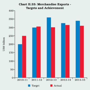 II.6.4 Amongst the major sectors, petroleum
products, oil meals, electronic goods, iron ore and
gems & jewellery dragged down the overall export
performance in 2014-15 (Chart II.34). While the fall
in exports of petroleum products reflected the
softening of international crude oil prices in the last
three quarters of 2014-15, weakness in demand
for other commodity classes interacted with
domestic supply constraints related to infrastructure
and other inputs to hit non-oil exports. Destinationwise,
exports to China, the EU, Singapore, Japan
and Saudi Arabia suffered a larger setback in 2014-
15. Given greater trade integration, India’s trade seems to have become increasingly responsive to
global economic and financial conditions (Box II.6).
Box II.6
Trade Linkages and Elasticities
India’s cross-border trade linkages have strengthened over
time. Not only has India diversified its exports in terms of
destinations, but its participation in global value chains
(GVCs) has also increased over the years, albeit at a lower
level than other peer economies (Chart 1), particularly in
chemicals and electrical equipment (OECD 2014).
Participation in GVC allows domestic firms to enter markets
by specialising in niche intermediate activities within a chain
and enables suppliers to upgrade production into highervalue
segments of their industries. This enhances
comparative advantages, productivity growth and
development levels in economies.
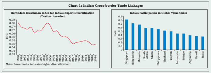 Greater cross-border linkages through GVCs also tend to
increase the sensitivity of trade to external business cycle
shocks (Gangnes et al. 2014). Since the world is gradually
transitioning to a stage in which GVC trade is assuming
more importance than it did before, there appears to have
been a long-run increase in the elasticity of global trade with
respect to world economic activity (Escaith et al. 2010). In
this context, estimation of country-specific trade elasticities
assumes importance, especially in an international
environment in which competitive monetary policy stances
and exchange rate effects have implications for export
competitiveness.
For India, the size of real exchange rate elasticity of real
non-oil exports is estimated to be in the range of 0.7 to 0.9
with a lag of less than one year, while the income elasticity
of real non-oil exports is 2.1 to 2.7 (Jain and Tewari. 2014).
Similarly, the volume of imports is found to be predominantly
responsive to domestic demand while its elasticity with
respect to the real exchange rate is broadly in the range of
0.3 to 0.5. The estimates of income and exchange rate
elasticities are broadly in line with other studies undertaken
for India (Table 1). Overall, there appears to be support for
the Marshall-Lerner condition implying the efficacy of
exchange rate changes in moving the trade balance to the
desired level.
In order to improve trade linkages with the rest of the world,
India’s participation in GVC must improve. Policy focus
should be concentrated on cluster development in particular
sectors with large presence of MSMEs so that they can
integrate effectively in the global production network.
Another way for domestic firms to integrate into GVC is
through a joint venture or strategic partnership to achieve
synergy gains. Cross-border foreign investments should be
encouraged. While inward FDI benefits domestic firms in
terms of capital, technology transfer and research and
development (R&D) capabilities, outward FDI increases
their productivity by providing access to scarce raw materials,
a skilled labour force and expanding production networks.
Firms also need to specialise in logistics, design, assembly
and R&D. Thus, further policy attention is warranted to
support in-house R&D so as to enable domestic firms to
achieve quality standards and specialise in high value added
activities. There is ample scope for improvement in the
quality and efficiency of services (for example, basic
infrastructure and air transport) which will help India raise its
share in GVC.
| Table 1: Major studies undertaken for India |
| Author (s) |
Findings |
| Hsing (2010) |
Marshall-Lerner condition holds |
| Aziz and Chinoy (2012) |
IE (4.0) and ERE (0.6) for exports |
| UNCTAD (2013) |
IE (1.9) and ERE (0.54) for exports |
| Pandey (2013) |
Marshall-Lerner condition holds |
| Mohan and Kapur (2014) |
ERE (0.21 to 0.65) for X and (0.19 to 0.42) for M |
| Raissi and Tulin (2015) |
IE (>1.5) |
| Note: X: Exports;
M: Imports;
ERE: Exchange rate elasticity;
IE: Income elasticity. |
Greater participation in GVC also makes a country’s trade
more susceptible to global economic and financial conditions
(that is, demand/supply conditions and exchange rate
changes). Given the sensitivity of India’s trade to income
conditions and exchange rate changes, policymakers need
to be cognizant of external shocks especially through capital
flows and domestic inflation and productivity levels as they
may have significant implications for real effective exchange
rate movements which eventually impact India’s trade
balance.
References:
Aziz, Jahangir and Sajjid Chinoy (2012), ‘India: More Open
Than You Think’, Economic Research, J.P.Morgan.
Escaith, Hubert, Nannette Lindenberg, and Sébastien
Miroudot (2010), ‘International Supply Chains and Trade
Elasticity in Times of Global Crisis’, Economic Research
and Statistics Division Staff Working Paper 2010-08, World
Trade Organisation, Geneva.
Gangnes, Byron S., Alyson C. Ma and Ari Van Assche
(2014), ‘Global Value Chains and Trade Elasticities’, UHERO
Working Paper No. 2.
Hsing, Y. (2010), ‘Test of the Marshall-Lerner Condition for
Eight Selected Asian Countries and Policy Implications’,
Global Economic Review, 39 (1): 91-99.
Jain, Rajeev and Soumasree Tewari, ‘Estimation of Export
and Import Functions for India’, Forthcoming, RBI Working
Paper.
Kapur, Muneesh and Rakesh Mohan (2014), ‘India’s Recent
Macroeconomic Performance: An Assessment and Way
Forward’, IMF Working Paper No.14/68.
Pandey, Ritesh (2013), ‘Trade Elasticities and the Marshal
Lerner Condition for India’, Global Journal of Management
and Business Studies, 3 (4): 423-28.
Raissi, Mehdi and Volodymyr Tulin (2015), ‘Price and Income
Elasticity of Indian Exports - The Role of Supply-Side
Bottlenecks’, IMF Working Paper No. 15/161.
OECD (2014), India Policy Brief, November.
UNCTAD (2013), Impact of the Global Slowdown on India’s
Exports and Employment. New York and Geneva: United
Nations.
Merchandise Imports
II.6.5 The plunge in global prices of crude oil by
nearly 50 per cent between June 2014 and March
2015 compressed India’s POL import bill by 16 per
cent yielding a saving of US$ 26.5 billion in relation
to the outgo on this account a year ago. Global
crude oil prices stayed modest in Q1 of 2015-16
(Chart II.35). Gold imports, however, recorded an
increase in terms of both value (20 per cent) and
volume (38 per cent) in response to a surge in
demand in H2 of 2014-15. The uptick in gold imports
in the later part of 2014-15 could largely be
attributed to festival demand, permission to trading houses to import gold for domestic consumption
as well as the withdrawal of the 20:80 scheme and other restrictions for gold imports.7 Further, sharp
increase in gold imports in March and April 2015 also reflected suppressed demand in preceding
months in anticipation of a cut in customs duty in
Union Budget 2015-16 and demand surge on
account of Akshaya Trithiya. After being subdued,
gold imports again spiked in the month of July 2015,
as gold prices dipped to the lowest level in last four
years, stimulating domestic consumption demand
(Chart II.36).
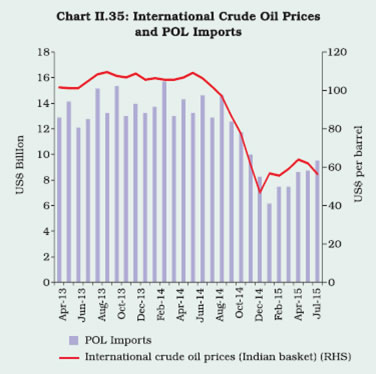
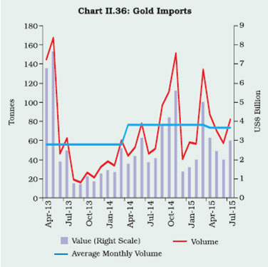 II.6.6 Non-oil non-gold imports picked up
modestly in 2014-15 largely in response to
domestic requirements of industry (Chart II.37).
Higher imports of iron and steel, iron ore, coal,
non-ferrous metals, chemicals and machinery also
resulted from shortfalls in domestic production in
certain sectors. In particular, the rise in coal imports
reflected higher requirements of power companies
which have added capacity to meet growing
domestic demand for power. Import of vegetable
oils was also driven by shortages in domestic
production. Non-oil non-gold imports increased in
the current financial year up to July 2015, though
at a modest pace.
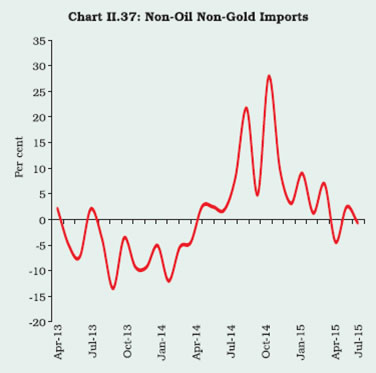 II.6.7 With the decline in exports exceeding the
fall in imports, the merchandise trade deficit
widened marginally in 2014-15 from its level in
2013-14. While softening of oil prices compressed
India’s POL trade deficit, the non-POL trade deficit
widened from US$ 34.2 billion in 2013-14 to US$
55.7 billion in 2014-15 (Table II.13). However, the
trade deficit at US$ 45.0 billion during first four
months (April-July) of 2015-16 was lower than that
in the same period of 2014-15.
| Table II.13: Merchandise Trade Deficit |
| (US$ billion) |
| Item |
2014-15 (P) |
2013-14 (R) |
| Value |
% Growth |
Value |
% Growth |
| 1 |
2 |
3 |
4 |
5 |
| Export |
310.5 |
-1.2 |
314.4 |
4.7 |
| Of which: |
|
|
|
|
| POL |
57.0 |
-9.7 |
63.2 |
3.8 |
| Non-oil |
253.5 |
0.9 |
251.2 |
4.9 |
| Imports |
447.5 |
-0.6 |
450.2 |
-8.3 |
| Of which: |
|
|
|
|
| POL |
138.3 |
-16.1 |
164.8 |
0.4 |
| Gold |
34.4 |
19.9 |
28.7 |
-46.7 |
| NONG |
274.8 |
7.0 |
256.7 |
-5.9 |
| Trade Deficit |
-137.0 |
|
-135.8 |
|
| Of which: |
|
|
|
|
| POL |
-81.3 |
|
-101.6 |
|
| Non-POL |
-55.7 |
|
-34.2 |
|
| Memo Item: |
|
|
|
|
| Trade Deficit as
% of GDP |
-6.7 |
|
-7.2 |
|
Source: DGCI&S.
Note: P: Provisional, R: Revised, POL: Petroleum, Oil, Lubricants.
NONG: Non-oil non-gold |
Current Account Deficit
II.6.8 The merchandise trade deficit (BoP basis)
was partly offset by a rise in net exports of services. Aided by better growth in the US, higher technology
adoption and the strength of the US dollar against
the rupee, India’s software exports seemed to have
benefitted, though appreciation of the rupee against
the euro and sluggish demand might have
dampened software exports to the euro area. Net
exports of travel services recorded a decline largely
due to higher payments on account of personal
services availed for education, medical reasons
and holidays. Notwithstanding the fall in international
oil prices, the flow of remittances remained stable.
II.6.9 India’s current account deficit (CAD) shrank
to1.3 per cent of GDP in 2014-15 from 1.7 per cent
a year ago. Holding the CAD at a sustainable level
going forward will hinge on a turnaround in
merchandise exports. This will also involve
assigning priority to unlocking domestic supply-side
bottlenecks in terms of infrastructure and other key
inputs, including through active policy interventions
to restore productivity and competitiveness across
a broad spectrum of leading sectors (Box II.7).
Box II.7
India’s New Foreign Trade Policy 2015-20
On April 1, 2015, the Ministry of Commerce and Industry
announced the Foreign Trade Policy 2015-20 (FTP) with a
vision to making India a significant participant in world trade
by 2020 and to enable the country to assume a leadership
position in the international trade discourse. FTP links rules,
procedures and incentives for exports and imports with
other initiatives (for example, Make in India, Digital India and
Skill India) with a view to improving ‘ease of doing business’
in India. The salient features of FTP are:
• To increase India’s exports of merchandise and
services from US$ 465.9 billion in 2013-14 to US$ 900
billion by 2019-20 and to raise India’s share in world
exports from 2 per cent to 3.5 per cent during this
period.
• A new scheme, the Merchandise Exports from India
Scheme (MEIS) aimed at the simplification of the
incentive structure, replacing multiple schemes is in
place.
• A new scheme, the Services Exports from India
Scheme (SEIS) with expanded scope is in place,
which will benefit all ‘service providers located in India’
instead of only ‘Indian service providers’.
• Allowing transferability and greater flexibility in using
‘duty credit scrips’ which exporters will get under MEIS
and SEIS.
• Prioritisation of sectors which have domestic
manufacturing capabilities and potential demand (for example, drugs and pharmaceuticals, chemicals and
electronics) where exports need to grow significantly to
achieve overall growth targets.
• Other sectors identified with great export potential
include engineering, leather, textiles, medical devices,
natural resource based items, gems and jewellery, agri
products and defence equipment.
• Emphasis on the need to increase India’s participation
in global supply chains. Adoption of the ‘whole-ofgovernment’
approach as a significant step towards
better coordination with state governments/other
departments.
• Indication of the revival of the interest subvention
scheme for exports from identified sectors for a period
of three years, though sectoral coverage and rate of
interest subvention are not indicated.
• Envisages a move towards paperless working in a 24x7
environment to facilitate the ease of doing business in
India.
Under the new FTP, the government has expanded the
scope of the new schemes to special economic zones
(SEZs). Even though the target set for 2019-20 for exports of goods and services appears achievable, demand conditions
in major trade partner economies will have to be supportive
and domestic bottlenecks (both in terms of infrastructure
and policy) need to be eased significantly. If the world
economy grows faster during 2015-19 than in the 2009-
14 period as projected by the IMF (2015), India’s exports
may fare better than in previous years. Nonetheless, taking
exports to the level of US$ 900 billion by 2019-20 will need a
higher compound annual rate of growth (CARG) of about 14
per cent during the FTP period (2015-16 to 2019-20) which
could be a challenge (Chart 1).
Financing of CAD
II.6.10 During 2014-15, India became a preferred
destination for private capital flows, which responded to improved perceptions of fundamentals, optimism
engendered by a stable government at the centre
and expectations surrounding resurgence of
business sentiment in an improved climate for
investors, both foreign and domestic. The abundance
of global liquidity in view of unconventional
monetary policies in advanced economies also
emerged as a push factor driving a relentless
search for returns. Non-debt creating capital inflows
alone far exceeded the financing requirement
(Chart II.38). Foreign portfolio investors brought in
about US$ 41 billion to Indian equity and debt
markets, making India the most attractive destination
among emerging markets. Further, net foreign
direct investment (FDI) inflows picked up strongly
in response to initiatives that are geared towards a
better business environment with policy certainty.
In particular, policy measures have been undertaken
with regard to easing of norms for FDI in certain
sectors, allocation of natural resources, the subsidy regime, financial inclusion, employment and job
creation for the youth and an improved and nonadversarial
tax administration. FDI inflows to India,
excluding disinvestments, were the highest after 2008-09 (Chart II.39). FDI mainly flowed into the
manufacturing sector responding to the
government’s ‘Make in India’ initiative, followed by
financial services, retail and wholesale trade. Within
the manufacturing sector, transport equipment and
chemical sectors were the major recipients and accounted for about 50 per cent of the total FDI in
2014-15. Inflows to NRI deposits and in the form of
external commercial borrowings were moderate
during 2014-15 relative to the preceding year,
signifying policy induced inflows in the past. With
net capital inflows exceeding CAD sizeably, there
was net accretion to reserves to the tune of US$
61.4 billion on a BoP basis (that is, excluding
valuation effects).
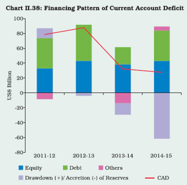
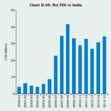 External Sustainability
II.6.11 External vulnerability indicators improved
significantly in 2014-15 on account of both a lower
accretion to the external debt stock and the build-up
of foreign exchange reserves. Key debt and
reserve-related indicators of external vulnerabilities
reflected an improved ability to discharge external
obligations. While the import cover ratio rose to 8.9
months as at end-March 2015, the ratio of shortterm
debt (by original as well as residual maturity)
to reserves and the ratio of total external debt to
reserves declined over the same period
(Table II.14).
| Table II.14: India’s External Sector Vulnerability Indicators |
| (Per cent unless indicated otherwise) |
| Indicator/Ratios |
End-Mar
2011 |
End-Mar
2012 |
End-Mar 2013 |
End-Mar 2014 |
End-Mar 2015 |
| 1 |
2 |
3 |
4 |
5 |
6 |
| 1. External Debt to GDP ratio |
18.2 |
20.9 |
22.3 |
23.6 |
23.8 |
| 2. Short-term to Total Debt (Original Maturity) |
20.4 |
21.7 |
23.6 |
20.5 |
17.8 |
| 3. Short-term to Total Debt (residual maturity) # |
40.6 |
40.9 |
42.1 |
39.6 |
38.9 |
| 4. Concessional Debt to Total Debt |
14.9 |
13.3 |
11.1 |
10.4 |
8.8 |
| 5. Reserves to Total Debt |
95.9 |
81.6 |
71.3 |
68.2 |
71.8 |
| 6. Short-term Debt to Reserves |
21.3 |
26.6 |
33.1 |
30.1 |
24.8 |
| 7. Short-term Debt (residual maturity) to Reserves # |
42.3 |
50.1 |
59.0 |
57.4 |
54.2 |
| 8. Reserves Cover of Imports (in months) |
9.5 |
7.1 |
7.0 |
7.8 |
8.9 |
| 9. Debt-Service Ratio |
4.4 |
6.0 |
5.9 |
5.9 |
7.5 |
| 10. External Debt (US$ billions) |
317.9 |
360.8 |
409.4 |
446.3 |
475.8 |
| 11. Net International Investment Position (NIIP) (US$ billion) |
-207.0 |
-264.7 |
-326.7 |
-336.8 |
-363.0 |
| 12. NIIP/GDP ratio* |
-12.1 |
-14.4 |
-17.8 |
-17.8 |
-18.1 |
| 13. CAD/GDP ratio |
2.8 |
4.2 |
4.8 |
1.7 |
1.3 |
| Note: #: RBI estimate; *: Based on US$ terms. |
Exchange Rate Movements
II.6.12 The US dollar gained significantly against
most international currencies during the year. The
Indian rupee, however, depreciated only marginally
against the US dollar; therefore, by the same token,
it gained strongly against other major currencies,
viz., euro, GBP and Japanese yen, reflecting the
weak economic outlook for these economies and
their ultra-accommodative monetary policies.
Reflecting persisting inflation differentials and
appreciation of the rupee in nominal terms vis-à-vis
India’s major trade partners, the real effective
exchange rate of the rupee during 2014-15, on
average, appreciated by 6.1 per cent and by 5.5
per cent (y-o-y) for the basket of 6 and 36 currencies
respectively. The rupee exchange rate also
witnessed lower volatility in 2014-15 and 2015-16
so far than in the earlier period (Chart II.40).
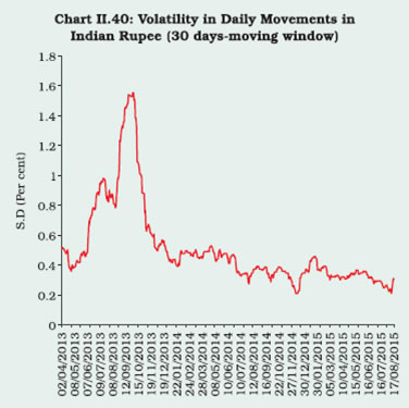 II.6.13 Going forward, external sector sustainability
will need close monitoring, especially in a global
environment characterised by high volatility in
financial markets, asynchronicity in monetary
policies of major advanced economies and in
particular, the widely expected lift-off of US interest
rates, and still high geo-political risks. Although
international crude oil prices stayed at modest
levels in Q1 of 2015-16 and dropped sharply in
August 2015 due to excess supply and subdued
demand, continuation of benign conditions for the
remaining part of the year still remains uncertain.
II.6.14 For India, every US$ 1 increase in
international crude prices broadly translates into
an increase in the net POL import bill by US$ 1
billion. Second, following the withdrawal of gold
import related measures, the import demand for
gold seems to be bouncing back as evident from a
growth (volume terms) of 38.5 per cent in 2014-15
and 34.3 per cent in April-July 2015. Third, key to
ensuring the viability of the external sector in this
backdrop is a renewed thrust on exports in terms
of both products and markets. Export diversification
has provided a means of insulation in the face of
sluggish global economic conditions and this should
be vigorously pursued to strengthen resilience and
to minimise the spillovers of external shocks.
|