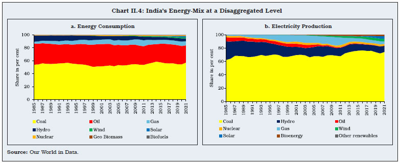
India’s diverse topography makes it highly vulnerable to climate risks, manifested in the form of sustained rise in temperature, erratic monsoon patterns, and rising frequency and intensity of extreme weather events. India’s goal of becoming an advanced economy by 2047 and achieving the net zero target by 2070 would require accelerated efforts in terms of reducing the energy intensity of output as well as improving the energy-mix in favour of renewables. Scenario analysis suggests that delayed climate policy actions could be costlier, in terms of larger output losses and higher inflation. Sectoral analysis, for risk mitigation, suggests policy interventions to focus on high emission-intensive sectors to minimise trade-off costs. 1. Introduction II.1 Climate change has moved to the centre stage of global public policy debate today because of its devastating macroeconomic impact, being experienced in recent years and the potential for harsher consequences in the future. The research focus accordingly has advanced from initial ‘detection and attribution’1 to ‘impact assessment and mitigation policies’. While growing scientific evidence has made it possible to forge a consensus2 on the key aspects of climate change – i.e., global warming is real and that human activities are a significant cause – the rising incidence of climate events across the globe has raised public awareness about this risk. II.2 Existing research work not only highlights the probable demand-side implications of climate change, but also supply shocks in the medium-to long-run with the potential to cause widespread disruptions to the overall macroeconomic and financial system. For example, the manifestation of climate change through changes in temperature and precipitation patterns along with the rising frequency and intensity of extreme weather events has implications for growth and inflation, with multiple channels of risk transmission. Sectoral implications could include disruptions in cropping cycles and variations in agricultural yield/output. In the industrial sector, there could be an increase in operational costs reducing profitability, owing to the imposition of new climate-friendly regulations, reduced utilisation of old stock of capital and diversion of investment towards greener infrastructure/capital/technology coupled with relocation of production processes and activities due to climate-related losses. Adversities for the services sector could be diverse, such as strains on financial services, say due to an increase in insurance claims, as well as disruptions in travel, transportation and business services. Climate events could also have implications for various factors of production. At a broader level, there could be implications for the labour market in terms of labour productivity decline due to climate-related health hazards, and climate migration, i.e., out-migration from areas that are significantly prone to climate risks to lesser affected regions. Capital could also be impacted due to physical loss of infrastructure that may depress return on capital and regulatory charges differentiating between green and other assets. Overall, costs are expected to rise for the economy owing to rehabilitation measures and new investment for mitigation and adaptation, which if funded by the government, could entail additional fiscal costs. II.3 Therefore, while the risks from climate change have generally been classified into two categories – physical risk and transition risk, the channels of risk transmission may be three: (i) direct impact or first-order effects; (ii) indirect impact or second-order effects; and (iii) spillover effects (intra-economy and cross-border impact or contagion risks) [BCBS, 2021; Ciccarelli and Marotta, 2021]. The direct transmission channels originate in sectors which are exposed to climate events more than others, whereas the indirect transmission channels involve the effects arising from sectoral value chains at various levels. It is through the indirect transmission channels that the impact of the climate event may spread to the whole economy. The third channel involves spillovers of impact arising from the interactions between the real economy and the financial sector. It would also involve implications for international trade and capital flows and through them for cross-border contagion risks. While the consensus as of now seems to suggest that the direct effects are likely to increase gradually over time across the globe as global temperature rises, what is still lurking in the shadow is the extent of the impact; the underlying non-linearities; and the timeline over which the impact may materialise (BCBS, 2021). This is more so because it is extremely difficult to obtain precise and reliable estimates of the overall macroeconomic impact of climate change, which are conditional upon not only the nature and magnitude of the climate shock, but also on how economies adapt and mitigate the impact through various policy actions. While there is a broader consensus on green transition as a common goal, the path to its achievement is rugged involving not only balancing known and unknown macroeconomic trade-offs, in particular growth-inflation-financial stability, but also creating a global environment for cooperation to drive joint actions to deal with the common challenge. II.4 From the perspective of monetary policy, an assessment of climate-related risks – the likely persistence of the impact of the shock, the extent of the impact on target variables and the transmission channels, and future risks – becomes important to insulate the economy from adverse consequences as monetary policy seeks to stabilise the economy after it is hit by unanticipated shocks. It has also been argued that climate change is not merely another market failure but presumably “the greatest market failure the world has ever seen” (Stern, 2006). The other side to the debate is the paradox that “success is failure” (Carney, 2016), implying that rapid and ambitious policy measures over a short-term horizon may not be desirable from the perspective of larger macroeconomic and financial stability. Therefore, from the standpoint of monetary policy, this calls for a careful monitoring and assessment of the visible patterns of climate-related risks and their associated implications for the economy, such that appropriate and timely policy measures may be calibrated. II.5 Against this backdrop, India is at the cusp of a unique development challenge. With India’s greenhouse gas (GHG) emissions3 increasing over four-fold during 1970 to 20214, a green transition path calls for a careful long-term planning and well-defined implementable strategies. More so because India is ranked seventh in the list of most affected countries in terms of exposure and vulnerability to climate risk events in 2019 as per the Global Climate Risk Index 2021 (Eckstein, et al., 2021). Hearteningly, India is also the highest ranked G-20 country as per the Climate Change Performance Index 2023 (Burck, et al., 2022; PIB, 2022). Both high climate risk exposure of the country and lead performance in mitigating risks pose challenges for estimating the macroeconomic impact of climate change in India. II.6 Accordingly, the key motivations of this chapter are to: (i) assess the impact of climate change on the Indian economy, and (ii) explore the future macroeconomic implications through scenarios linked to India’s Nationally Determined Contribution (NDC) commitments. In comparison to a baseline scenario (business as usual [BAU]), a modest green transition scenario (characterised by continuation of remarkable achievements of the past decade) and an ambitious green transition scenario (with the required rate of reduction in emissions consistent with achieving the net zero target by 2070) bring to the fore the often discussed temporal trade-offs between environmental and macroeconomic objectives. These assessments are done taking into account available facts and India-specific peculiarities of the climate-economy nexus. For instance, India’s monsoon-dependent agriculture, economically significant long coastline and energy-intensive industrial sector highlight the challenges posed by climate risks. II.7 Set against these key motivations, this chapter is organised under seven sections: Section 2 provides the geographical and structural characteristics of the Indian economy. It analyses why climate change presents India with a unique and daunting challenge in terms of its emission targets vis-à-vis the aspiration for higher economic growth. Section 3 discusses the various forms in which climate change risks manifest in India. Section 4 provides a macroeconomic impact assessment of climate change in India, especially with regard to the physical risks. Section 5 analyses various scenarios of green transition consistent with the country’s potential to become an advanced economy by 2047 alongside achieving the net zero emissions target by 2070, while highlighting the underlying growth-inflation trade-offs that may emerge from pursuing both economic and environmental goals. Sector specific green transition challenges are elucidated in Section 6. Section 7 presents concluding remarks with some policy suggestions. 2. India’s Exposure to Climate Risks Geographical Features II.8 India’s high vulnerability to climate events is on account of its unique geographical features and economic structure. The Indian sub-continent has a diverse topography ranging from the snow-clad Himalayas in the north, fertile plains and the deltaic region in the east, long coastline of more than 7500 kilometres covering 9 states from the east to the west in the mainland forming the southern peninsula, and the Thar desert in the north-west (Chart II.1). This diverse topography is not only exposed to different temperature and precipitation patterns, but also makes it vulnerable to extreme weather events posing wide-ranging spatial and temporal implications for the economy. 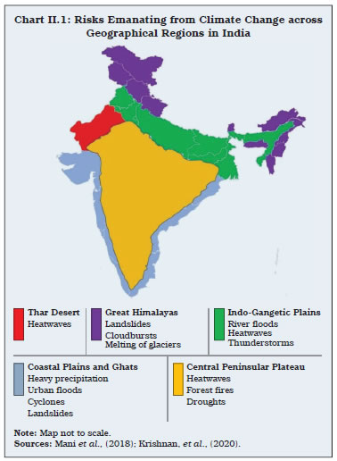 II.9 For instance, India’s long coastline, also referred to as the coastal plains, features among the most densely populated regions of the world, primarily owing to its fertile soil and accessibility to ports. The coastal plains provide important hinterlands to some of the major ports of the country. Therefore, from a macroeconomic standpoint, India’s long coastline assumes significant importance. On the other hand, global warming leaves the coastal plains susceptible to flooding owing to rising intensity and frequency of extreme sea level events, in the form of tides, waves, storm surges and rise in mean sea level. Moreover, risks from global warming also include loss of land and receding coastlines due to coastal erosion, impacting coastal infrastructure, human settlement, and industrial and farm activities. Coastal cities are prone to cyclones and also face acute dangers of frequent flooding and salinisation of farmlands and freshwater supplies (Krishnan, et al., 2020). Economic Structure II.10 India’s sectoral composition of GDP is skewed towards services sector, which is globally considered to be emission-light with relatively lower energy intensity of output. Share of services sector in GVA increased from 43.2 per cent during 1980s to 60.9 per cent during 2010s (Chart II.2a). In contrast, the share of agriculture in overall GDP fell from 38.5 per cent to 16.3 per cent over the same period, while that of the industrial sector remained broadly unchanged at a little over one-fifth of overall GVA. The services-led growth path since 1980s was associated with a declining trajectory in overall CO2 emissions growth for about twenty years till early 2000s (Chart II.2b). There was a brief episode of acceleration in CO2 emissions growth which took place between 2004-05 to 2009-10, which could be attributed to the spurt in manufacturing activity observed during that period. CO2 emissions growth started decelerating around 2011-12 and followed a declining trajectory again during the decade of 2010s. II.11 A deep-dive into India’s sectoral break up shows that metal industries, electricity and transports, owing to their dependency, both direct and indirect, on fossil fuels, are the highest emission-intensive5 sectors, together accounting for around 9 per cent of India’s total GVA in 2018-196 (Table II.1). In contrast, wholesale and retail trade, financial and professional services, including information and computer related services, professional, scientific and technical services, comprising more than 27 per cent of India’s overall GVA, are among the relatively low emission-intensive sectors. Although industrial sector emissions are higher as compared with agriculture and services sectors, emission intensity of agriculture sector, which involves both energy related emissions and non-energy related emissions (such as N2O and CH4) is, in fact, higher than certain industries such as textiles, machinery and equipment as well as construction activity. Thus, the sectoral composition of the Indian economy – smaller share of the industrial sector and prevalence of low energy-intensive services – helps contain India’s emissions. 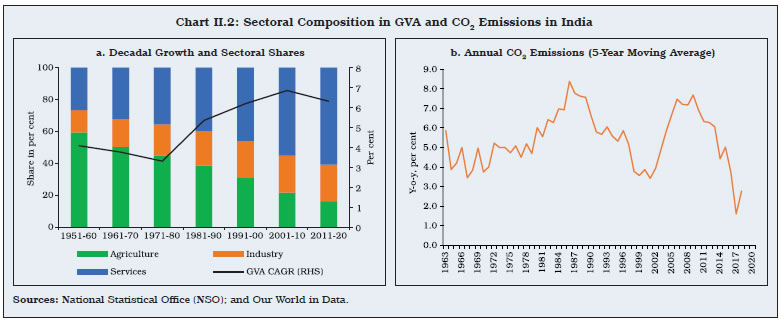 II.12 With energy production driving around three-quarters of global GHG emissions, changing the energy-mix – away from non-renewables to renewables – is critical. In terms of the overall energy-mix, fossil fuel-based energy sources, viz., coal, oil and natural gas, continue to dominate energy consumption in India (Chart II.3). At a disaggregated level, within fossil fuels, coal is the major source followed by oil (Chart II.4a). The share of coal in India’s electricity production is around 60 per cent (Chart II.4b). 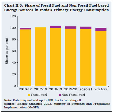
| Table II.1: Sector-wise Share in GVA and CO2 Emission Intensity (2018-19) in India7 | | Sector | Share in GVA | CO2 Emission Intensity (Metric Tons of CO2 Emissions per US$ 1 Million of Output) | | Agriculture, forestry and fishing | 14.8 | - | | Agriculture, hunting, forestry | 13.8 | 84.7 | | Fishing and aquaculture | 1.0 | 4.1 | | Mining | 2.6 | - | | Mining and quarrying, energy producing products | - | 382.1 | | Mining and quarrying, non-energy producing products | - | 185.2 | | Manufacturing | 18.3 | - | | Food products, beverages and tobacco | 2.0 | 11.9 | | Textiles, apparel and leather products | 2.4 | 37.8 | | Metal products | 2.6 | 2796.6 | | Machinery and equipment | 4.6 | 67.0 | | Electricity, gas, water supply and other utility services | 2.3 | - | | Electricity, gas, steam and air conditioning supply | - | 7263.8 | | Water supply; sewerage, waste management and remediation activities | - | 110.4 | | Construction | 8.1 | 26.1 | | Wholesale and retail trade; repair of motor vehicles | 12.3 | 67.8 | | Accommodation and food services | 1.1 | 22.0 | | Transport | 3.9 | - | | Air transport | 0.07 | 1210.4 | | Land transport | 4.0 | 378.8 | | Water transport | 0.1 | 1587.7 | | Financial, real estate, ownership of dwelling and professional services | 22.5 | - | | Financial services | 6.0 | 27.4 | | Real estate and ownership of dwellings | 6.5 | 48.6 | | Professional services | 8.9 | 127.9 | | Public administration and defence | 5.7 | 16.1 | | Other services | 7.1 | - | | Education | 3.7 | 23.2 | | Arts, entertainment and recreation | 0.3 | 31.8 | | Human health and social work activities | 1.5 | 17.5 | | Other service activities | 1.6 | 77.4 | -: denotes categories for which data are not reported.
Sources: NSO; and IMF Climate Change Dashboard. |
 3. Manifestation of Climate Change in India II.13 Major indicators that signal about climate-related stress are distinct temperature and precipitation anomalies. India has witnessed these anomalies quite frequently in recent years. While annual average temperature in India has been increasing gradually, the rise has been significantly sharp during the last vicennial than during any other 20-year time interval since 1901 (Chart II.5). In terms of minimum and maximum temperatures, during 1901-2021 the annual mean temperature showed an increasing trend of 0.63 degree Celsius per 100 years with a rise in the maximum temperature of 0.99 degree Celsius per 100 years. The rising trend in the minimum temperature was relatively lower than that in the maximum temperature, with minimum temperature increasing by 0.26 degree Celsius per 100 years (IMD, 2021) [Chart II.6].
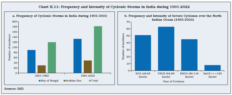
II.14 Such rapid changes in India’s temperature profile have led to the rising temperature anomaly8, as is also observed globally (Chart II.7). II.15 The past decade (2011-2021) has been an outlier in terms of major temperature irregularities from the normal trend. The decade has been the warmest on record with temperatures shooting up in the range of 0.34-0.37 degree Celsius above the long period average (LPA). Further, 11 out of the 15 warmest years in India since 1901 have occurred during 2007-2021. Moreover, 2022 and 2021 have been the fifth and the sixth warmest years on record since 19019, with the annual mean temperature up by 0.51 degree Celsius and 0.44 degree Celsius, respectively, above the 1981- 2010 average level. 2016 has been the warmest year on record so far for India since 1901, with a temperature anomaly of 0.71 degree Celsius above the 1981-2010 average. II.16 In 2022, with the onset of summer, temperature shot up above the normal across several regions in the country, especially in the northern states of Punjab, Haryana, Delhi, Rajasthan and Uttar Pradesh, with the range being 3 degree Celsius to 8 degree Celsius. March 2022 recorded the highest average maximum temperature with an anomaly of 1.9 degree Celsius above the normal10 and second highest mean temperature with an anomaly of 1.6 degree Celsius since 1901 for the month of March (Chart II.8). Additionally, April 2022 also recorded the second highest mean temperature for the month of April since 1901 (highest occurred in 2010). II.17 Such high temperature with the onset of summer led to severe heatwave conditions in the country with implications for agricultural output. For instance, the wheat crop in the rabi season of 2022 was adversely impacted, leading to lower production. Moreover, heatwaves also led to increased number of forest fires. By the end of April 2022, almost 70 per cent of India was affected by its spread (IMD, 2022). Moreover, during May 2022, the heatwave extended into the coastal and the eastern regions of the country. High temperatures recorded during the summer months adversely affected grain filling and caused early senescence, thus reducing foodgrain yields during the year. In 2023, India experienced the hottest February on record (in terms of maximum temperature), with the IMD predicting an enhanced probability of heatwaves occurring in the central and northwest regions of India during the summer of 2023. 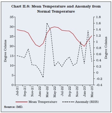 II.18 The precipitation pattern in a region is heavily conditional on its geographical characteristics.11 In this regard, a dominant feature of the Indian sub-continent is the south-west monsoon (SWM) season (June-September), also referred to as the Indian summer monsoon. Around 75 per cent of India’s annual rainfall is concentrated during the four months of the SWM season, which is vital for the agricultural output during the kharif cropping season, as almost half of the country’s net sown area is still unirrigated. Further, rainfall during this season is important to fill up the reservoirs in the country which helps in the much-needed irrigation during the rabi cropping season. Even though India has become self-sufficient in foodgrains, anomalies in SWM, whether temporal or spatial, impact food price dynamics and the inflation outlook. II.19 Over the years, the pattern of SWM season appears to have undergone subtle changes.12 Notably, while the average annual rainfall at the all-India level during the last vicennial (2000-2020) saw a rise over that during 1960-1999, over a longer time horizon since 1901, annual average rainfall in India has gradually declined. Importantly, the average rainfall received during the SWM season has declined by around 8 per cent during 2001-2020 as compared with that during 1941-1960. Moreover, evidence suggests that while dry spells have become more frequent during the last several years, intense wet spells have also increased. During 2019-2022, the overall rainfall in the country has been higher than the LPA but its distribution, including the pre- and the post-monsoon seasons, has been skewed. For instance, in 2019, the post-monsoon rainfall turned out to be 30 per cent higher than the LPA, whereas in 2020 the pre-monsoon rainfall surpassed the LPA by 21 per cent (Chart II.9). In 2021, both the pre-monsoon and the post-monsoon seasons recorded rainfall higher than the LPA, at 18 per cent and 44 per cent, respectively. Further, in 2022, although the annual rainfall was 108 per cent of its LPA, there were significant spatial dispersion in rainfall during the SWM season. For instance, the south peninsular and central regions of India received above normal rainfall (122 per cent and 119 per cent higher than their LPA, respectively). In contrast, the north-western parts of India received just normal rainfall (101 per cent of its LPA), whereas the north-eastern parts of the country received below normal rainfall (82 per cent of its LPA). 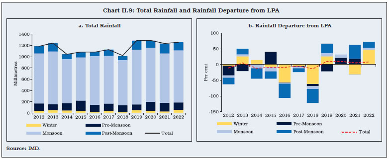 II.20 Over the years, the SWM season has also seen onset and withdrawal dates shifting, with the withdrawal being generally delayed and often coinciding with the north-east monsoon or the winter monsoon season (Table II.2). For instance, during 2019, despite a delayed onset (June 8, 2019) and a highly deficient phase during June (33 per cent below LPA), the monsoon season ended with a 10 per cent above normal rainfall, which was the highest recorded rainfall in the past 25 years (the highest during the period 1990-2019 being 12.5 per cent in 1994). | Table II.2: Onset and Withdrawal of Monsoon in India | | Year | Date of Arrival | Delay in Arrival | Date of Withdrawal from India | Delay in Withdrawal | | 2012 | 5 June | 4 days | 18 October | 3 days | | 2013 | 1 June | 0 days | 21 October | 6 days | | 2014 | 6 June | 5 days | 27 October | 12 days | | 2015 | 5 June | 4 days | 19 October | 4 days | | 2016 | 8 June | 7 days | 28 October | 13 days | | 2017 | 30 May | (-)2 days | 25 October | 10 days | | 2018 | 29 May | (-)3 days | 21 October | 6 days | | 2019 | 8 June | 7 days | 16 October | 1 days | | 2020 | 1 June | 0 days | 28 October | 13 days | | 2021 | 3 June | 3 days | 25 October | 10 days | | 2022 | 29 May | (-) 2 days | 23 October | 8 days | | Source: IMD Annual Reports. | II.21 Climate change is also being manifested in the form of rising intensity and frequency of extreme weather events such as excessive/ unseasonal rainfall (often leading to floods), severe temperature fluctuations (e.g., heat waves and cold waves) and high wind speeds (e.g., cyclones). Since the early 2000s, extreme weather events have been very frequent in India. For instance, unseasonal rainfall and heatwaves have become a regular phenomenon (Chart II.10). While Maharashtra, Karnataka, Uttar Pradesh and Madhya Pradesh have witnessed frequent unseasonal rains over the years, states such as Rajasthan, Haryana, Punjab, Delhi, Uttar Pradesh and Jharkhand have been the most impacted by heatwaves with the onset of summer and in the pre-monsoon months. II.22 Moreover, the frequency of cyclonic storms has increased in India over the years (Chart II.11a).13 For instance, as compared with the normal of 11-12 cyclonic disturbances and 4.8 cyclonic storms observed in the North Indian Ocean (NIO) during 1960-2020, there were 8 cyclonic storms during 2019. Importantly, their intensity has also increased with a greater number of very severe cyclonic storms (VSCS) and extremely severe cyclonic storms (ESCS) as compared with severe cyclonic storms (SCS) (Chart II.11b). In 2021, out of the five cyclonic storms that occurred, one was ESCS (Tauktae) and another was VSCS (Yaas) in May (pre-monsoon season) over the Arabian Sea and the Bay of Bengal, respectively. 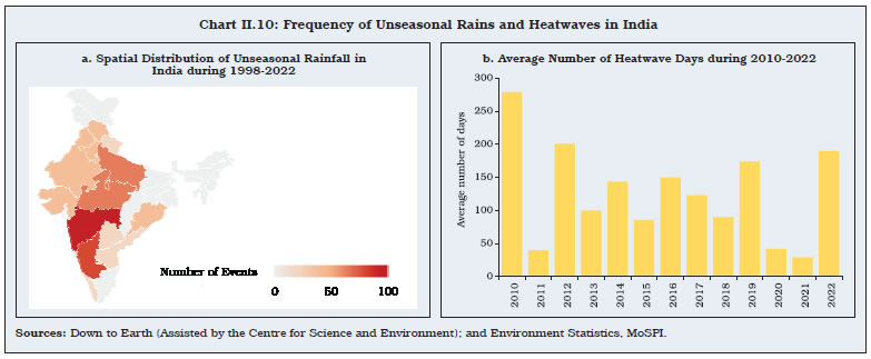
 II.23 The distribution of cyclones between the east coast and the west coast has also changed over the years with increased frequency of cyclonic storms over the Arabian Sea (Ghosh et al., 2021). Historically, cyclones in the Arabian Sea were fewer as compared with that in the Bay of Bengal. During 2019, out of the 20 cyclonic disturbances/storms that occurred, a majority of them were in the Arabian Sea (west coast) [IMD 2019].14 A spatial distribution of severe cyclones reveals that the number of cyclones that occurred in the states of Odisha, Andhra Pradesh and Tamil Nadu in the eastern coast of India during 1961-2022 was much higher than that during 1901-1960 (Chart II.12). Additionally, in the west coast, the incidence of SCS in Gujarat increased significantly during 1961-2022 as compared with Maharashtra and Goa. An increase in the frequency of ESCS over the Arabian Sea and the NIO has been attributed to anthropogenic warming (Murakami et al., 2017). 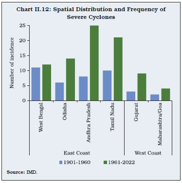 II.24 Additionally, the incidence of droughts and floods has also seen a rise in the recent years. Floods and droughts are generally classified as hydroclimatic extremes. In India, the number of droughts has seen a spike, with their severity being higher during 1961-2021 as compared with the period 1901-1960 (Ghosh et al., 2021). In particular, central India and southern peninsula regions are more prone to droughts. Among the coastal states, Karnataka and Maharashtra are the major states that have witnessed a higher frequency of droughts during 1951-2021 (Chart II.13). Further, as per the UN Office for Disaster Risk Reduction, the number of floods in India shot up to 90 during the decade of 2006-2015 as compared with 67 during 1996 to 2005. Frequent floods are one of the significant contributors to the average annual losses in India in economic terms from climate related disasters (World Bank, 2021). Studies have indicated that anthropogenic geographical alterations, including incessant unplanned urbanisation, to be one of the prime reasons behind the rising number of city floods in India (Yang et al., 2015; Liu and Niyogi, 2019; Krishnan, et al., 2020). 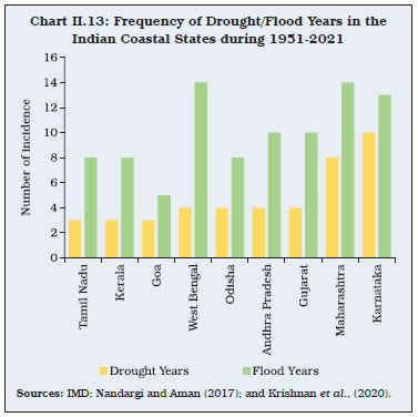
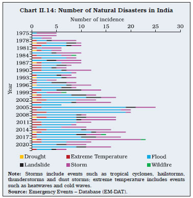 II.25 Overall, India is relatively more exposed to floods and storms (i.e., cyclones and hailstorms) than droughts and heatwaves (Chart II.14). Such incidences pose significant risks to agricultural production (Krishnan, et al., 2020) and food price volatility (Dilip and Kundu, 2020; Ghosh et al., 2021; and Kishore and Shekhar, 2022). 4. Macroeconomic Impact of Climate Change in India II.26 The impact of climate change on the economy could manifest through its adverse impact on the supply potential of the economy as well as by altering demand conditions. Climate change events are often characterised as adverse supply shocks, which reduce the economy’s aggregate output and raise prices, thus posing adverse implications for the potential growth of the economy. Further, uncertainty following a climate change event also adds to the volatility in both output and prices. Changing weather patterns may also impact consumer behaviour and preferences, thus influencing demand conditions (Andersson et al., 2020; Ciccarelli and Marotta, 2021). II.27 Fighting climate change could also cause a global inflation shock (Morison, 2021), exacerbating the output-inflation trade-offs faced by central banks and increasing risks to medium-term price stability (Schnabel, 2021). The potential impact of climate change mitigation policies on energy production and prices could be adverse (Volz, 2017). II.28 The impact of physical and transition risks on the economy could be direct, indirect and through spill-over effects (Illustration II.1). Physical risk drivers are often categorised into two types: acute risks – related to the occurrence of extreme weather events, and chronic risks – associated with gradual shifts in temperature and precipitation patterns (McKinsey Global Institute, 2020; NGFS, 2022b), though acute risks can also arise due to chronic risks. For example, a rise in global temperature may lead to acute changes in the climate by causing heatwaves and wildfires (Jones et al., 2020; Abatzoglou et al., 2019). Further, a warmer atmosphere can hold more moisture, leading to an increase in heavy and concentrated rainfall in several regions (IPCC, 2018). These could impact overall output as acute climate events such as destructive flash floods cause physical damages to properties, infrastructure and crops. II.29 Transition risk drivers, on the other hand, are the economy-wide changes arising from the transition towards a low-carbon economy. These may relate to the public-sector policies; innovation and technologies; or investor and consumer sentiments/preferences facilitating a greener economy. Therefore, the impact of a climate-related transition risk would be conditional upon a host of factors and would involve multiple underlying dependencies relating to the climate-economy nexus. The impact is also more indirect than physical risk. 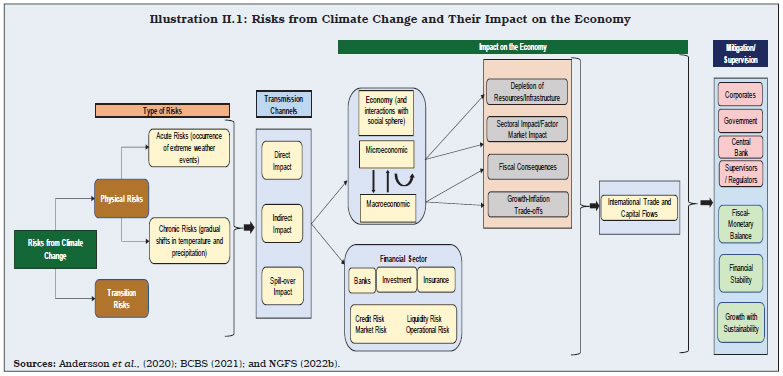 II.30 Multiple channels through which climate change impacts the Indian economy has been documented in the literature, which is still evolving. India, being among the top 10 economies in terms of vulnerability to climate risk events, is already witnessing the adverse impact of climate change on its people’s lives and livelihood. For instance, in 2019, India lost nearly US$ 69 billion due to climate related events, which is in sharp contrast to US$ 79.5 billion lost over 1998-2017 (UNISDR, 2018). Floods in India during 2019 affected nearly 14 states causing displacement of around 1.8 million people and 1800 deaths. Overall, around 12 million people were impacted by the intense rainfall during the monsoon season in 2019 with the economic loss estimated to be around US$ 10 billion. Additionally, the SWM rains in recent years have often been accompanied by significant temporal and spatial dispersions causing crop damages, thereby leading to higher food inflation and its volatility (Dilip and Kundu, 2020; Ghosh et al., 2021). II.31 The IPCC Working Group (WG)-II (IPCC, 2022b) report states that India is one of the most vulnerable countries globally in terms of the population that would be affected by the sea level rise. By the middle of the present century, around 35 million people in India could face annual coastal flooding, with 45-50 million at risk by the end of the century (World Bank, 2021). Further, the agriculture sector and fisheries would face significant adverse consequences due to the rising sea level and ground water scarcity. Literature indicates that most of India has been experiencing adverse effects of temperature on living standards, as the households most affected are dependent primarily on the agriculture sector for their livelihood (Mani et al., 2018). Further, the incidence of flash flooding is expected to increase, if global temperature soars to 2 degree Celsius above the pre-industrial levels (Ali and Mishra, 2018). In terms of ecosystem services, around 600 million of India’s population are facing severe water stress, with 8 million children below 14 years in the urban India at risk due to poor water supply (Niti Aayog, 2019). II.32 India, along with countries such as Brazil and Mexico, face high risk of reduction in economic growth, if global warming raises temperature by 2 degree Celsius as against 1.5 degree Celsius (IPCC, 2018). Climate change manifested through rising temperature and changing patterns of monsoon rainfall in India could cost the economy 2.8 per cent of its GDP and depress the living standards of nearly half of its population by 2050 (Mani et al., 2018). India could lose anywhere around 3 per cent to 10 per cent of its GDP annually by 2100 due to climate change (Kompas et al., 2018; Picciariello et al., 2021) in the absence of adequate mitigation policies. Furthermore, Indian agriculture (along with construction activity) as well as industry are particularly vulnerable to labour productivity losses caused by heat related stress (Somnathan et al., 2021). India could account for 34 million of the projected 80 million global job losses from heat stress associated productivity decline by 2030 (World Bank, 2022). Further, up to 4.5 per cent of India’s GDP could be at risk by 2030 owing to lost labour hours from extreme heat and humidity conditions. Moreover, heatwaves could also last 25 times longer, i.e., rise in severity, by 2036-2065 if current rate of carbon emissions is not contained (CMCC, 2021). These estimates, thus, underscore the importance of timely adoption and faster implementation of climate mitigation policies to reduce the adverse impact on the Indian economy. II.33 Despite the rising frequency of extreme weather events, India has been reporting record production of foodgrains and horticulture in recent years, reflecting a faster growth in rabi production (Chart II.15). As most of the excess and unseasonal rainfall events and cyclones take place during the monsoon or post-monsoon seasons, their impact on kharif crop is more than on rabi crop in terms of crop loss. Consequently, the impact of climate change on inflation through the production channel appears to be mild at the aggregate level due to geographically well-distributed foodgrains production as well as the localised nature of climate events. 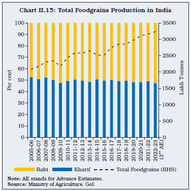 II.34 In contrast, horticulture crops, especially perishables like vegetables, are more exposed to extreme weather events, such as cyclones and unseasonal rainfall during the post monsoon period, thereby temporarily impacting their prices (Kishore and Shekhar, 2022). For example, inflation in onion prices shot up to 327 per cent in December 2019 led by unseasonal rains; potato prices by 107 per cent in November 2020 due to unseasonal rains; and tomato prices by 158 per cent in June 2022 due to heatwave and cyclone led crop damages. In fact, even with a low share of these three vegetables (Tomato, Onion, Potato – TOP) in CPI (2.2 per cent), they contribute a large part of the volatility in food and headline inflation (Chart II.16). Of late, farmers are also adapting to such climate events by adjusting their sowing and harvesting schedules, while R&D in agriculture has focused on developing climate resilient crops to minimise the adverse impact on food production, prices and farmers’ income. 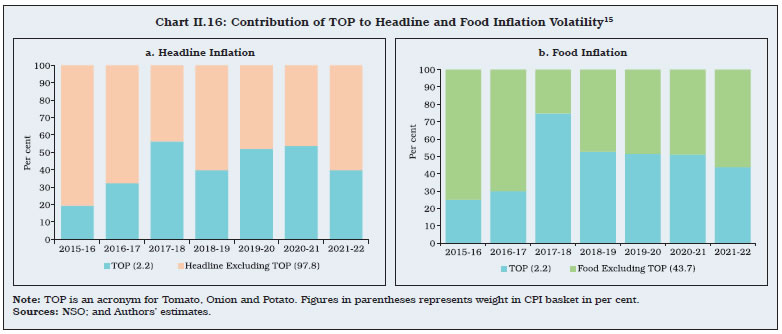 II.35 Overall, the impact of changing temperature and precipitation patterns on the agricultural sector is highly non-linear and manifests with a greater intensity for non-irrigated regions in extreme circumstances. Estimates indicate that when a district experiences unusually high temperature (in the top 20 percentile of the temperature distribution), there is a 4 per cent reduction in agricultural yield during the kharif season and a 4.7 per cent reduction during the rabi season (GoI, 2018). Similarly, when a district receives significantly less rainfall than usual (in the bottom 20 percentile of the rainfall distribution), there is a 12.8 per cent decrease in kharif yield and a smaller, yet noticeable decrease of 6.7 per cent in rabi yield. With the rising anthropogenic emissions, the frequency of such extreme events could increase even further, with implications for agriculture yield, farmers’ income and food inflation. II.36 Set against this backdrop, the macroeconomic impact of some of the key extreme weather events, such as floods, cyclones and droughts has been analysed in the context of India during the last 10 years, i.e., 2012-13 to 2021-22. Similar to Ghosh et al., (2021), 5 states along the western coastline (Gujarat, Maharashtra, Goa, Karnataka and Kerala) and four states along the eastern coastline (West Bengal, Odisha, Andhra Pradesh and Tamil Nadu) together with their eight neighbouring inland states have been considered. Difference-in-difference (D-i-D) panel data regression results indicate that natural disasters adversely impact economic activity, i.e., lower output growth, while raising inflation (Table II.3).16 The result contrasts with some of the earlier studies that suggest an increase in the GDP due to the post disaster investment and multiplier effects (Caballero and Hammour, 1994). Further, the results do not indicate a negative impact on agricultural GVA.17 While India has attained a degree of self-sufficiency with respect to food production, Government policy interventions towards developing climate-resilient crops and changing cropping pattern - such as introducing drought/flood/temperature tolerant varieties in paddy and pulses especially in the coastal states; water-saving paddy cultivation methods, advancement of rabi planting dates in areas with heat stress; and community nurseries as solutions for delayed monsoon arrival - have played a major role in increasing the resilience of India’s agriculture sector against climate related stress (NICRA, 2016). With regard to inflation, literature indicates that the impact of extreme weather events is generally short-lived (Freeman et al., 2003; NGFS, 2020; Dilip and Kundu, 2020; Ghosh et al., 2021), although heterogenous with respect to the type of the hazard, and varies between advanced and developing economies (Parker, 2018). Nonetheless, the fact that inflation and its volatility are driven by such shocks that make predicting the short-term inflation path difficult, pose major challenge for the conduct of forward-looking monetary policy. The results do not indicate a statistically significant rise in capital expenditure in the coastal states during the calamity year, instead there is an indication that the overall capital expenditure falls18 when a calamity hits, thus substantiating the fall in economic growth. Further, a need would also arise for relief and rehabilitation/reconstruction measures in the period following a natural disaster, which would require diversion of budgeted funds, thus having implications for the Government’s fiscal deficit. | Table II.3: Difference-in-Difference Panel Data Results | | D-i-D Coefficients | Inflation | GSDP | NSDP Per Capita | GSVA Agriculture | NSVA Agriculture | GSVA Manufacturing | NSVA Manufacturing | GSVA Services | NSVA Services | CAPEX | | | (1) | (2) | (3) | (4) | (5) | (6) | (7) | (8) | (9) | (10) | | C | 7.34*** | 5.01*** | 3.24*** | 10.69*** | 11.72*** | 2.58 | 1.97 | 6.08*** | 4.09*** | 20.94*** | | | (1.93) | (0.87) | (0.80) | (2.30) | (2.58) | (1.88) | (2.06) | (0.79) | (0.63) | (4.53) | | γ | -0.29 | 1.99* | 2.85** | -7.89*** | -9.06*** | 8.17*** | 10.40*** | 1.03*** | 1.99* | -4.34 | | | (0.35) | (1.12) | (1.11) | (2.42) | (2.72) | (2.51) | (2.99) | (0.30) | (0.99) | (5.22) | | δ | -2.19 | 1.19 | 1.27 | -9.60*** | -11.26*** | 6.03 | 7.13*** | 1.36 | 2.20*** | -9.03* | | | (1.93) | (1.05) | (0.98) | (2.77) | (3.04) | (2.17) | (2.71) | (0.81) | (0.80) | (4.63) | | βDID | 1.04** | -2.71** | -2.73** | 8.32*** | 10.06*** | -11.43*** | -14.03*** | -1.31** | -2.80** | 4.63 | | | (0.44) | (1.24) | (1.23) | (2.93) | (3.21) | (2.71) | (3.40) | (0.56) | (1.06) | (5.75) | Note: ***, **, * represent significance at 1 per cent, 5 per cent and 10 per cent levels, respectively.
Figures in parentheses indicate robust standard errors. | II.37 While the above analysis helps in assessing the extent of the impact of extreme weather events on some of the key macroeconomic indicators at the all-India level, it would also be interesting to examine the impact of one particular climate event on household-level indicators of economic well-being. An analysis using household-level data from the National Sample Survey Organisation (NSSO) reveals evidence of adverse effects on consumption, with the median household experiencing a fall in consumption by 16 per cent (Aggarwal, 2019). The rising incidences of cyclones in India are of significant concern of late as they are inflicting massive loss to infrastructure, life and property in and around the coastal states. While the loss of life from cyclones has come down over the years19 due to better disaster management, early warning systems, and resilient infrastructure such as cyclone shelters, the economic loss has often been unavoidable as was evident in the case of cyclone Amphan (Box II.1). Box II.1
Economic Impact of Cyclone Amphan on the Coastal Districts of West Bengal and Odisha The super cyclonic storm Amphan was a natural disaster that originated in the Bay of Bengal and affected the coastal districts of West Bengal and Odisha in India and the adjoining Bangladesh in May 2020. The economic impact of cyclone Amphan on the coastal districts of West Bengal and Odisha is compared vis-à-vis their non-coastal neighbouring districts. While the coastal districts of West Bengal and Odisha have been used for estimating the treatment effect (economic impact) of the cyclone, their adjoining non-coastal districts that lie within 100 kilometres from the eastern coast of India are used for the comparison purpose. In order to examine the impact of the cyclone on economic activity, following Bayer et al., (2022) the difference-in-difference (D-i-D) panel data regression method is used. Further, economic activity has been represented by an array of measures, such as household consumption, district level deposit and credit, and employment demand under the Mahatma Gandhi National Rural Employment Guarantee Act (MGNREGA). For empirical estimation, RBI’s district-level credit and deposit data available at quarterly frequency during Q3:2019-20 to Q4:2020-21, monthly data on household-level expenditure and its sub-categories during January-December 2020 available from the Consumer Pyramids Household Surveys (CPHS) database maintained by the Centre for Monitoring Indian Economy (CMIE), and monthly data on the number of households that worked and those that demanded work under the MGNREGA20 during January-December 2020 from the MGNREGA Public Data Portal maintained by the Ministry of Rural Development, GoI, are used. The following equation is estimated to study the impact: where, In (ydt) represents the log of the dependent variables, where d and t denote district and time, respectively. The above equation is also run with district level and month/quarter level fixed effects instead of the Treatedd and Postt variables, while keeping the variable (Treatedd * Postt) unchanged. Results of the regression analysis are presented in Table 1. The results indicate an increase in credit in districts affected by the cyclone, implying that firms and households need to finance disaster related rehabilitation/restoration expenses. This can come either from their own savings or by borrowing from the financial institutions, but the results show no significant change in savings. Moreover, a significant decline in food consumption is observed, especially when district and time fixed effects are accounted for. This may be due to the need for reconstruction following cyclone-induced damages, with the reconstruction dependent on bank credit and/or the fund received under post-cyclone rehabilitation schemes of the Government. On rural employment side, a decline is observed in the employment demand under MGNREGA. This decline could be because of temporary migration post cyclone, as Amphan displaced approximately 5 million people. | Table 1: Difference-in-Difference Regression Results | | D-I-D Coefficients | Credit
(₹ crore) | Deposit
(₹ crore) | Total Consumption
(₹) | Food Consumption
(₹) | MGNREGA Employment
(Person days) | | β with Post and Treated | 0.037** | 0.004 | 0.012* | -0.007 | -0.346 | | | (0.077) | (0.007) | (0.009) | (0.006) | (0.318) | | β with Time and District fixed effects | 0.037** | 0.004 | -0.006* | -0.022*** | -0.346*** | | | (0.018) | (0.440) | (0.008) | (0.007) | (0.078) | Note: ***, **, * represent significance at 1 per cent, 5 per cent and 10 per cent levels, respectively.
Figures in parentheses indicate robust standard errors. | To sum up, the results indicate that natural disasters or one-off extreme weather events such as Amphan could lead to a rise in district-level credit offtake following the occurrence of the event, which may be used for rebuilding and rehabilitation. Therefore, an increased frequency of such natural disasters could increase debt levels of both firms and households in the high-risk regions. Reference: Beyer, R., Narayanan, A. and Thakur, G. (2022). Natural Disasters and Economic Dynamics: Evidence from the Kerala Floods. Policy Research Working Paper No. 10084, World Bank. | II.38 Moreover, for a holistic understanding of the economic impact of climate change, it is also imperative to look beyond average macroeconomic impact and understand various dimensions of distributional consequences. Impact on different sectors could be distinct depending on the nature of activity. Irrigated areas may be wealthier and, at the same time, less vulnerable to rising temperatures. Ownership structure of agricultural assets, not only land but also human capital, could influence return on assets and thus, condition households’ response to climate events. II.39 Another dimension of climate change could be individuals’ response to climate events by way of geographical relocation. Evidence based on the all-India Census at the inter-state level reveals that climate related shocks have a significant impact on bilateral migration across states (Dallmann and Millock, 2017). For instance, drought frequency and severity in the origin state increases out-migration, especially for states with relatively higher share of agriculture in total output. Further, inter-state migration is also influenced by both agricultural income and total income in the destination state relative to the state affected by the climate event. 5. India’s Transition Towards Net Zero21 II.40 The IPCC has recognised that the challenges faced due to global warming are mainly on account of the cumulative historical and current GHG emissions of the developed countries. However, the cumulative impact has been assessed to be iniquitous with the developing countries bearing the brunt of climate change even as they may be constrained by their limited capacity to respond to its challenges (IPCC-Working Group III, [IPCC, 2022a]). Given the cataclysmic consequences of global warming, it is imperative, however, to reduce GHG emissions by both developed and developing countries alike. Emerging market and developing countries, including India, face the additional trade-off that they must continue to prioritise their own growth and developmental aspirations, while pursuing their climate related nationally determined goals. Against this backdrop, scenarios have been developed in this section on India’s roadmap to net zero by 2070 conditional on different assumptions for real GDP growth on the one hand, and changes in the share of green energy in total energy demand as well as changes in the energy intensity of the GDP on the other to explain the nature of policy trade-offs involved. II.41 Overall, carbon emission is a product of population and CO2 emissions per person. This can be decomposed into four factors following the ‘Kaya Identity’22 (Kaya, 1997). These include (i) Population; (ii) Income (GDP per capita); (iii) Energy intensity of GDP and (iv) Carbon intensity of energy; wherein (iii) and (iv) are determined by technology.23 The Kaya Identity is expressed as:  II.42 In India, like most other countries, a large-scale increase in GDP stood out to be the key driver of emissions – a stronger driver than the increase in population (Chart II.17). Within the technology factor, India was able to reduce its energy intensity of GDP steadily overtime by bringing both structural changes in the economy and technological efficiency. The pace of decline in energy intensity took a leap in early 2000s. The decline has continued in the recent years as well. In contrast, the emission intensity of energy has increased, especially in the last decade (2011 onwards). Although overall emission intensity of GDP (product of energy intensity of GDP and carbon intensity of energy) has declined, further improvement is required to ensure a declining path of emissions in alignment with India’s NDC. As maximum feasible expansion of GDP is necessary, technology would have to play a key role in India’s net zero transition. This would involve a combination of more efficient energy-mix and technological advances in the industrial sector leading to lower emission intensity of GDP. Empirical evidence based on cross-country studies broadly suggests that an increase in the share of renewable energy in total energy consumption can have a significant impact in reducing GHG emissions provided the share of renewables in total energy consumption is sufficiently high (Chen et al., 2022; Hao, 2022). In the Indian context, based on the emission factors of different sources of energy obtained from the IPCC Emission Factor Database, it has been estimated that a one per cent increase in the share of renewable energy in the energy-mix reduces CO2 emissions by around 0.63 per cent. This contributes positively towards achieving the NDC target. Alternative scenarios relating to the future path of GHG emissions have been developed to measure the viability of achieving net zero emissions by 2070, while balancing the dual objectives of achieving high growth and mitigating climate risks. 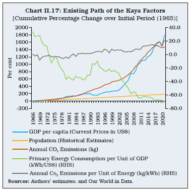 II.43 The baseline scenario assumes that the Indian economy will continue to grow at its past trend rate, i.e., compound annual growth rate (CAGR) of real GDP achieved during the past decade (2011-12 to 2019-20) of 6.6 per cent, without any action taken towards meeting the commitments under its NDC (Table II.4). Moreover, UN’s population projections for India are used and it is also assumed that the energy intensity of GDP defined as total primary energy consumption per unit of GDP24 would continue to decline by 2.3 per cent annually (the annual average rate of decline as observed during 2011-12 to 2019-20). Furthermore, total carbon sequestration from various types, such as biological, which refers to storage of carbon in grasslands, forests, soil and oceans; and technological, such as creating carbon capture, usage and storage (CCUS), is assumed to remain at the 2016 level of 0.3 gigatonne, with no further enhancements. Under these baseline assumptions, net emissions would continue to rise over time, widening the gap from net zero target, which underscores the need for active policy interventions to close the gap and move to the target (Table II.5). | Table II.4: Scenario Assumptions | | Variables | Baseline | Alternate Scenario 1 | Alternate Scenario 2 | Alternate Scenario 3 | | Real GDP Growth | CAGR of 6.6 per cent
(realised during 2011-20) | 6.6 per cent | 9.6 per cent during 2023-24 to 2047-48 and 5.8 per cent thereafter | 9.6 per cent during 2023-24 to 2047-48 and 5.8 per cent thereafter | | Decline in Energy Intensity of GDP | CAGR 2.3 per cent
(realised during 2011-20) | Gradually raised | CAGR 2.3 per cent | Gradually raised | | Carbon Absorption Capacity in the Economy | 0.3 gigatonne
(realised in 2016) | Raised to 3.3 gigatonnes | 0.3 gigatonne (realised in 2016) | Raised to 3.3 gigatonnes | Notes: 1. The required rate of decline in energy intensity increases gradually to 5.9 per cent during 2031-32 to 2040-41 and tapers off to around 5.3 per cent by 2070 in alternate scenarios 1 and 3.
2. The decadal share of green energy in alternate scenario 1 (alternate scenario 3) increases from around 5.5 per cent in 2021-22 to 9.1 in 2030-31 and thereafter increases rapidly to around 70 per cent (82 per cent) by 2070-71.
3. Emission factors for green and non-green energy sources have been assumed to be 0.0 gigatonnes per tera-watt hour and 0.00029 gigatonnes per tera-watt hour, respectively, based on data available for total emissions and energy-mix from Our World in Data. | II.44 The first alternate scenario (scenario 1) assumes that India will maintain its past trend GDP growth (6.6 per cent), while adhering to its immediate objectives under the NDCs – reducing emission intensity and expanding the share of renewable sources in electrical energy to 50 per cent by 2030, as well as the long-run objective of the net zero emission by 2070. Achieving net zero by 2070, however, would require even higher levels of energy efficiency which could be achieved only through a sharper decline in energy intensity of GDP over the decades, besides a more efficient energy-mix. This would require the annual rate of decline in energy intensity to increase gradually from its current level of 2.3 per cent to 5.0 per cent by 2070. At the same time, the share of green energy in total energy consumption would need to reach to about 70 per cent by 2070 from around 5.5 per cent25 in 2021-22.26 Furthermore, this scenario remains compliant with the declared NDC target of enhancing natural carbon sink capacity by about 3 gigatonnes by 2030 along with efforts towards expanding forest and tree cover. Achievement of net zero under this scenario would lead gross GHG emissions to peak by 2032-33 and decline thereafter to deliver net zero GHG emissions by 2070. The level of energy consumption by 2070 would be 1.8 times higher than that of 2021-22 level as against 7.2 times higher under the baseline (BAU) scenario. | Table II.5: Energy Transition and GHG Emissions Towards Net Zero by 2070 vis-à-vis 2021-22 | | Scenarios | Gross GHG Emissions Level by 2070
(Gigatonnes) | Rate of Change in Emissions
(Per cent) | Rate of Reduction in Emission Intensity
(Per cent) | Rate of Reduction in Energy Intensity
(Per cent) | | Cumulative | CAGR | Cumulative | CAGR | Cumulative | CAGR | | Baseline | 19.2 | 469.4 | 3.6 | -73.0 | -2.7 | -67.6 | -2.3 | | Scenario 1 | 3.3 | -1.0 | -0.02 | -95.7 | -6.2 | -91.9 | -5.0 | | Scenario 2 | 32.4 | 859.6 | 4.7 | -75.2 | -2.8 | -67.6 | -2.3 | | Scenario 3 | 3.3 | -1.5 | -0.03 | -97.5 | -7.2 | -92.1 | -5.1 | Note: Gross GHG emissions for India at 2021-22 was 3.4 gigatonnes.
Source: Authors’ Estimates. | II.45 A second alternate scenario (scenario 2) assumes that India would achieve a higher growth trajectory to become an AE by 2047. The per capita income threshold defined by the IMF for country-group classification of ‘Advanced Economies’(AEs), ‘Emerging Market Economies’ (EMEs) and Low-Income Developing Countries’ (LIDCs) has been used to estimate the required level of GDP by 2047-48. As per this classification, India currently belongs to the group of EMEs (per capita GDP at US$ 2,450 in 2022-23) and its per capita GDP would have to cross the estimated threshold27 of US$ 33,632 in 2047-48 for it to become an AE. This translates into a required annual real GDP growth of 9.6 per cent between 2023-24 to 2047-48. With respect to climate goals, however, the BAU assumption is maintained as in the baseline. Higher growth together with no environmental commitments would translate into even higher trajectory of energy requirement and emissions leading to deviation further away from net zero target by 2070. Under this scenario, total primary energy requirement and net GHG emissions are estimated to be 12.5 times and 10.5 times higher, respectively, as compared with their levels in 2021-22. II.46 The third alternate scenario (scenario 3) accommodates the twin-objectives of becoming an AE by 2047 and achieving the net zero target by 2070. This requires an even more aggressive effort as compared with the targets stated under its current NDCs in terms of both energy intensity and energy-mix. Under this scenario, the annual rate of decline in energy intensity would need to increase to 5.4 per cent and the share of green energy in total energy consumption would have to increase to about 82 per cent by 2070 (Chart II.18). The implied level of energy consumption by 2070 would be 3.1 times higher as compared with 2021-22 level.  II.47 According to the Climate Action Tracker (CAT), an independent scientific project that tracks government climate action plans across countries,28 India’s updated NDCs, which include reducing emission intensity of its GDP by 45 per cent by 2030; achieving 50 per cent cumulative electric power installed capacity from non-fossil fuel-based energy resources by 2030; and creating an additional carbon sink of 2.5 to 3 billion tonnes of CO2 equivalent through additional forest and tree cover by 2030, will not be sufficient to meet the level of reductions needed for limiting global warming to 1.5°C. With its updated NDCs, India’s fair share rating nevertheless improved from “highly insufficient” to “insufficient” (CAT, November 15, 2022) [Chart II.19]. II.48 There is also an alternate view that the effective way to combat climate change is not by sacrificing growth rather to let nations grow so that they would have more resources for abatement and shifting to greener technology (Schelling, 1992). The Economic Survey 2023, GoI also recognised that continued development may be the best defence against climate change as securing external funding could be difficult. Such growth strategies, however, may conflict with environmental objectives in the medium- to long-run. Therefore, a more balanced approach, wherein the trade-off of maximising growth without compromising on the environmental commitments, is called for (Box II.2). 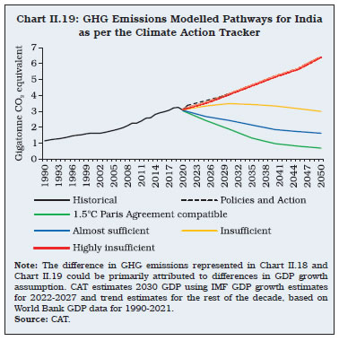
Box II.2
Economic Growth, Energy Consumption and Emissions: The Trade-offs Given the debate on growth and GHG emissions trade-off, a simple environmental Solow-type growth model (Solow, 1999; Xepapadeas, 2005) is presented here to simulate the per capita real GDP scenarios for the Indian context under different levels of energy usage and their corresponding GHG emissions. Higher per-capita GDP should normally require higher energy. But, using this framework, it is identified and showed that suitable changes in technology and energy-mix can achieve the dual objective in a less costly manner. A standard production function as follows is considered: Using this framework, the steady-state is solved for a given E and then various scenarios are simulated under different levels of energy input (E) and energy-mix for the Indian context. Given the baseline parameter specifications (Table 1), the growth rate of the economy is estimated as 6.6 per cent. This growth rate, however, does not enable India to attain the per capita income level of an AE by 2047. | Table 1: Parameter Specification of the Model | | Parameters | Observed Value | Sources | | Capital income share (α1) | 0.67 | KLEMS | | Labour income share (α2) | 0.3 | KLEMS | | Energy cost share (α3) | 0.03 | KLEMS | | Labour augmenting technology growth (ɡ) | 7.1% | KLEMS | | Population growth (n) | 1.01% | World Bank | | Depreciation rate (δ) | 0.1 | Banerjee and Basu (2019) | | Savings rate (s) | 0.31 | NSO | | Energy augmenting technology growth (b) | 2.6% | Estimated using World Bank Data | | Note: Labour income share, energy cost share and labour productivity are used from KLEMS data for manufacturing sector for the period 2011-12 to 2017-18. The capital income share is obtained as the residual. The savings rate is the average from 2011-12 to 2020-21. Energy augmenting technology growth represents the observed growth in the inverse of energy intensity of GDP during 2011-12 to 2019-20. | Therefore, an alternate scenario wherein India’s objective of becoming an AE by 2047 is considered. A scenario where the labour augmenting and energy augmenting technology growth rates are 10 per cent and 6 per cent, respectively, the output elasticity of energy at 0.06 and the labour income share at 0.64 (which resembles that of AEs)30 results in a growth rate of 9.4 per cent which meets the target of India becoming an AE by 2047 (Chart 1). In this scenario, the energy usage works out to be 1.9 times of the present level. To understand the effect of growth on GHG emissions under different combinations of energy-mix, the model further explores the contours of emission paths (Chart 2).31 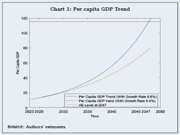 By increasing the share of green energy, it would be possible to achieve both the objectives of reducing emissions without compromising on the growth target. In this context, it is worthwhile to note that the commitment of NDC mandates that 50 per cent of the electrical energy must come from renewables by 2030. The estimates suggest that it is possible for India to become an AE by 2047-48 by having only 1.65 times GHG emissions as compared with the current level if 60 per cent of total energy usage is covered by greener sources. Going further ahead, if the economy continues to move in the direction of improving the energy-mix by having 85 per cent of energy from greener sources, it is also possible to reach net zero by 2070 while attaining the per capita income level of AEs. Table 2 summarises the model results in terms of emission and compares that with the results of the linear model presented earlier in this section. The growth model shows that the dual objective of net zero emission target and becoming an AE is possible with a lesser energy consumption as compared with the linear model. This is enabled by the assumed improvement in labour productivity and energy efficiency. 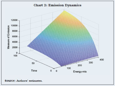 Overall, the analysis suggests that coordinated policy actions together with technological improvements and structural changes may be necessary for India to simultaneously meet its dual goals of becoming an AE with net zero emissions. | Table 2: Summary of the Emission Possibilities | | Key Results | 2021-22 | 2029-30 | 2047-48 | 2070-71 | | Linear Model | Growth Model | Linear Model | Growth Model | Linear Model | Growth Model | Linear Model | Growth Model | | Total energy consumption (Terrawatt/hour) | 9070.1 | 9070.1 | 14689.6 | 11060.1 | 27238.6 | 17904.0 | 27699.6 | 19047.0 | | Net emissions (Gigatonnes) | 1.7 | 1.7 | 1.8 | 1.1 | 3.6 | 1.8 | 0.0 | 0.0 | | Note: Net emissions are derived as total emissions less projected carbon absorptions as part of NDC: 1.5 gigatonnes in 2021-22; 3.1 gigatonnes by 2029-30 and 3.3 gigatonnes by 2047-48 which continues thereafter. Net emissions are also determined by the energy-mix, the path of which could be different across models. | References: Banerjee, S. and Basu, P. (2019). Technology shocks and business cycles in India. Macroeconomic Dynamics, Vol. 23(5), 1721-1756. Solow, R. M. (1999). Neoclassical Growth Theory. Handbook of Macroeconomics, 1, 637-667. Xepapadeas, A. (2005). Economic Growth and the Environment. Handbook of Environmental Economics, 3, 1219-1271. | II.49 The Network of Central Banks and Supervisors for Greening the Financial System (NGFS) has linked the standard integrated assessment models (IAMs) with a global macroeconomic model – referred to as the National Institute Global Econometric Model (NIGEM) – to produce policy insights over the short-run, wherein the framework considers both physical and transition risks from climate change. The NIGEM analyses the macroeconomic impact under six standard global scenarios (Annex II.1). 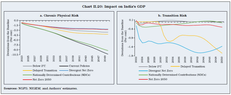 II.50 Taking into account the global NGFS scenarios, overall macroeconomic implications for India are illustrated through the NIGEM model. The model reveals that more the ambitious mitigation goals are at a global level, lesser would be the negative impact of physical risks on GDP vis-à-vis the baseline of no impact of climate change (best case scenario) [Chart II.20a]. However, the dynamics are different when transition risks are considered (Chart II.20b). The divergent net zero and delayed transition scenarios cause larger negative impact on GDP on account of temporal and sectoral imbalances in impact realisation and transmission. The other scenarios, i.e., ‘below 2°C’, ‘Net Zero 2050’ and ‘NDCs’ have broadly similar dynamics and lead to lower sacrifice of growth. Thus, in these scenarios, higher physical risk can cause a decline in GDP, by around 1 to 3 per cent from the baseline level in 2030. However, by 2047, the impact can be far more negative at around 3 to 9 per cent depending on the extent of risk mitigation. II.51 Since the economy is impacted by both types of risks, the combined effect needs to be visualised for policy insights (Chart II.21). Global scenarios of ‘current policies’ and ‘NDCs’ have the highest negative impact on output, mainly due to dominance of physical risk impact in the case of India. The reason for ‘NDCs’ having a more negative impact than ‘Net Zero 2050’ and ‘Below 2°C’ is that, whereas NDCs act as constraints on the individual countries, the other scenarios are comparatively more restrictive at the global level and thus, entail lower physical risk across countries over time. In essence, global commitments and coordination towards climate risk mitigation remains crucial, without which individual economies, including India, may be significantly impacted due to the possibility of globally inconsistent mitigation efforts and insufficiency of individual NDCs. 
 II.52 Physical and transition risks also impact inflation through macroeconomic linkages. In the case of physical risks, both inflation and its volatility increase over time, but the extent of increase is maximum under the scenarios of “current policies” and “NDCs” (Chart II.22a) [these scenarios also involve higher growth sacrifices as discussed earlier]. Since physical risks are expected to rise over time impacting aggregate supply, in the absence of sufficient risk mitigating measures, the impact on inflation is assessed to be more under lesser ambitious mitigation goals. In case of transition risks, however, inflation increases in the initial years owing to the imposition of carbon tax and other mitigation policies which raise the cost of production initially, but the impact gradually wanes towards the baseline, i.e., the deviation tends to zero (except for the delayed transition scenario) [Chart II.22b]. This could possibly be due to the falling cost of green transition over time on account of wider availability and adoption of technology32 as well as economic agents’ expectations getting progressively aligned with the nation’s transition path. II.53 Overall, the effect of climate risks on inflation is dominated initially by the impact of green transition before getting overwhelmed by physical risks (Chart II.23). This is because physical risks are expected to rise over time with climate change, whereas transition risks would take effect from the time when a risk mitigating policy is implemented. II.54 A comparative picture of the impact of physical risks and transition risks for EMEs like India with that of an AE like the US suggests that the adverse impact of climate change in India is significantly higher due to greater susceptibility to physical risks (Box II.3). II.55 Thus, in terms of the NGFS scenarios factoring in India’s NDC commitments, a transition towards a less carbon economy has a limited impact on growth and inflation. Therefore, while in the short-run, sticking to the ‘NDC scenario’ produces a minimal impact on India’s inflation, a delayed response can shoot up inflation over the medium-term. In terms of the impact on GDP, although the NDC commitments come with a greater negative impact for India due to its high sensitivity to physical risk, concerted efforts globally towards climate risk mitigation would significantly help smoothen green transitioning over time. II.56 Overall, how India’s carbon emission trajectory may evolve in future would depend on GDP growth and policy actions (in line with NDC or otherwise), and the trade-offs in the short-run versus medium-to long-run. First, as per the baseline – GDP growth of 6.6 per cent and no policy actions – GHG emission level will rise from 3.4 gigatonnes in 2021-22 to 4.5 gigatonnes in 2030-31 and further to 8.2 gigatonnes by 2047-48. Second, the current level of actions as per NDC commitments, will still be insufficient to achieve net zero by 2070. Net zero by 2070 calls for accelerated actions on top of NDC commitments such as (i) further reduction in energy intensity progressively by 2.8 per cent annually until 2030-31 and by around 5.5 per cent thereafter and (ii) increase in the share of green energy in primary energy consumption to 9 per cent by 2030-31, 27 per cent by 2047-48 and 70 per cent by 2070. This will result in rise in GHG emissions at a slower pace from the current level of 3.4 gigatonnes in 2021-22 to 4.2 gigatonnes in 2030-31 before declining modestly to 4.1 gigatonnes by 2047-48. Box II.3
Climate Change Impact on GDP – A Comparative Assessment Since the NGFS sets out differential targets for countries across the globe, with stricter restrictions especially for the AEs, the transition risk impact could be higher for them in the short-term. On the other hand, as the Indian economy is more vulnerable to physical risks from climate change (as elaborated in section 2) the impact may be more for India. Due to the higher sensitivity to physical risks as reflected in India’s high vulnerability ranking as discussed earlier, the Indian economy gets deeply impacted in the long-term under a lenient risk mitigation plan, i.e., under the scenarios of “current policies” and “NDCs”. Additionally, the impact on India is not too different from the global average, except under these two scenarios (Table 1). Moreover, India is different from most of the AEs in terms of the composition of energy basket, with the dominance of coal under fossil fuel, which could partly explain the differential impact. For example, in the case of the US, the energy-mix and electricity production structure are significantly different from India, with relatively higher use of renewables and non-coal based sources. | Table 1: Impact on GDP | Scenarios
(Deviations from Baseline in Per cent) | Impact on GDP
(USA) | Impact on GDP
(World) | Impact on GDP
(India) | | Below 2°C in 2030 | -1.93 | -1.67 | -1.91 | | Below 2°C in 2050 | -2.29 | -3.02 | -3.80 | | NDC in 2030 | -2.59 | -2.14 | -3.16 | | NDC in 2050 | -5.56 | -5.74 | -9.08 | | Current Policies in 2030 | -1.55 | -1.63 | -2.86 | | Current Policies in 2050 | -5.09 | -6.05 | -9.87 | | Source: NGFS, NIGEM. | Reference: NGFS. (2022a). NGFS Scenarios for Central Banks and Supervisors. | II.57 Second, the objective of becoming an AE by 2047 implies a higher annual GDP growth of 9.6 per cent, which would pose additional challenges for achieving the net zero target. With GDP growth of 9.6 per cent and no policy actions as above, GHG emission level may rise from 3.4 gigatonnes in 2021-22 to 5.5 gigatonnes in 2030-31 and further to 15.5 gigatonnes by 2047-48 and 32.4 gigatonnes by 2070-71. Under this scenario, achieving net zero by 2070 calls for even further accelerated actions than what was needed under 6.6 per cent growth rate. Over and above the NDC commitments, it would require (i) a sharper decline in energy intensity at the rate of 5.6 per cent per annum from 2031-32 (ii) increase in the share of green energy in primary energy consumption from around 5.5 per cent in 2021-22 to 9.1 per cent by 2030-31, 28.7 per cent by 2047-48 and around 82 per cent by 2070-71. II.58 An assessment of physical and transition risks using the global NIGEM-NGFS model suggests that under current policies, India’s GDP may be lower by 2.9 per cent from the baseline in 2030, and 8.7 per cent by 2047. With each country following their own NDCs, India’s GDP may be lower by 3.2 per cent from the baseline in 2030 and by 8.1 per cent by 2047, suggesting not much gain. However, a net zero by 2050 strategy instead of by 2070 results in lower loss of output – by 2.2 per cent from the baseline in 2030 and 3.2 per cent by 2047 – implying this may be a better policy option globally. As per current policies/ NDCs, the impact on inflation is expected to be minimal, even though its volatility is expected to increase. Overall, delayed and lenient policy actions generate adverse impact on both growth and inflation outlook in the medium-to long-run. 6. Sectoral Green Transition Challenges II.59 The impact of climate change could be different across sectors. Further, as sectors have different technology pathways for decarbonisation, a uniform approach may not be the best strategy. In view of the difficult policy trade-off between containing near-term adverse output impact by delaying policy actions versus larger output losses in the medium-run due to delayed policy actions, a sector-specific approach to climate risk mitigation can help in minimising the trade-off costs. A pragmatic approach would be to target those sectors i) which have higher contributions to the current levels of emissions, and ii) which are more amenable to mitigation strategies - both in terms of costs as well as marginal gains. II.60 In this context, four key sectors – electricity, mobility, industry and agriculture – have been identified which are responsible for the bulk of the GHG emissions in India. Within the industrial sector, the policy options and implications of decarbonisation in select hard-to-abate sectors such as steel, cement and chemical industries are specifically examined. The objective is to assess the current production structure and technology as well as the emerging trends in consumption so as to provide insights on how the envisaged transition path at the macro level can be realised. Electricity Sector II.61 For addressing climate change concerns on a sustainable basis, transforming the electricity sector will be crucial given that around 70 per cent of electricity in India is produced from thermal power plants. This makes the Indian electricity grids highly carbon-intensive among major economies (Chart II.24). II.62 India has embarked upon an ambitious plan of achieving 500 GW of total renewable energy capacity by 2030 and raising the share of renewable electricity generation to 50 per cent. One of the key factors that may help in facilitating this transition without a major increase in the cost to the overall macroeconomy will be the advancement in technology, which has led to notable fall in the prices of renewable energy in recent years. Globally, the price of electricity from solar and onshore wind has declined by 89 per cent and 70 per cent, respectively, during 2009-19 (UNDP, 2022). In India too, electricity tariffs are lower for solar and wind (Table II.6). 
| Table II.6: Electricity Tariff in India in 2021-22 | | Source | Tariff
(₹/kwh) | | Conventional (APPC)* | 3.85 | | Nuclear | 3.42 | | NHPC Ltd. | 3.36 | | Solar | 1.99 | | Wind | 2.44 | *Average Power Purchase Cost (APPC).
Note: The tariffs for solar and wind are the lowest tariffs discovered in various auctions conducted by Solar Energy Corporation of India (SECI).
Sources: Central Electricity Authority (CEA); NHPC; and SECI. | II.63 Globally, not a single fossil fuel plant features among the 20 cheapest power plants (Table II.7). Furthermore, the levelised cost of electricity (LCOE) generated from solar power and wind, including integration costs, is expected to fall further by around 40-55 per cent and 20-25 per cent, respectively, by 2030 (BP, 2022). This could propel the transition to a cleaner energy-mix. India has one of the largest synchronous inter-connected grids in the world which operates on one frequency to balance electricity demand and supply over a huge geographical area, making the task of adapting to variable renewable energy (VRE) sources relatively easier. However, massive investments are required in inter-state transmission systems (ISTS) to avoid congestion during peak hours. India plans to invest ₹2.8 lakh crore in ISTS for renewable energy evacuation by 2030 (The Economic Times, 2022b). Mobility Sector II.64 Mobility sector, with a share of around 14 per cent in India’s overall CO2 emissions, is the fastest growing source of emissions in India. A breakup of energy consumption and CO2 emission in this sector indicates that road mobility contributes the maximum to CO2 emission (Table II.8). | Table II.7: Plant Level Levelised Cost of Electricity (LCOE) Calculation | | Country | Plant Category | Total Capital Costs
(US$/MWh) | Operations and Maintenance Costs
(US$/MWh) | Fuel Costs
(US$/MWh) | LCOE
(US$/MWh) | | Sweden | Nuclear | 5.9 | 12.9 | 9.3 | 28.2 | | Denmark | Wind | 22.9 | 6.3 | 0.0 | 29.2 | | Switzerland | Nuclear | 7.4 | 12.9 | 9.3 | 29.6 | | France | Nuclear | 8.4 | 12.9 | 9.3 | 30.7 | | Norway | Wind | 20.9 | 9.8 | 0.0 | 30.8 | | USA | Nuclear | 5.2 | 18.7 | 9.3 | 33.3 | | Brazil | Wind | 27.6 | 6.0 | 0.0 | 33.6 | | France | Solar | 30.4 | 3.5 | 0.0 | 33.9 | | USA | Solar | 30.4 | 4.2 | 0.0 | 34.6 | | USA | Wind | 26.5 | 8.7 | 0.0 | 35.2 | | India | Solar | 31.9 | 3.7 | 0.0 | 35.6 | | India | Wind | 32.2 | 3.7 | 0.0 | 35.9 | Note: There is no fuel cost for wind and solar energy. The fuel cost for nuclear energy is assumed to be same across countries.
Source: International Energy Agency (IEA). | II.65 In terms of transport infrastructure, passenger kilometers (kms) and freight ton-kms in roadways have grown by 10 times and 5 times, respectively, during 2000-2017, whereas in the railways they have grown by 2.5 times and 2 times, respectively (Chart II.25). The Gati Shakti scheme launched by the Indian government to develop a multi-modal transportation system aims to integrate various modes of transport such as roads, railways, airways, and waterways to reduce logistics costs and improve efficiency. By improving the efficiency of the transportation system, the scheme will help reduce vehicular emissions and promote sustainable transportation. | Table II.8: Transport Sector - Energy Consumption and Emission (2019) | | | Energy Consumption
(Twh) | CO2 Emission
(Million tons) | | Road | 1144.0 | 292.9 | | Petrol | 337.8 | 87.5 | | Diesel | 691.4 | 184.5 | | Gas | 114.0 | 20.9 | | Aviation | 120.0 | 24.8 | | Railways | 43.7 | 22.7 | | Electricity | 20.0 | 16.4 | | Diesel | 23.7 | 6.3 | | Total | 1307.7 | 340.4 | | Sources: Energy Statistics of India; Indian Railways; PIB; and Authors’ estimates. | II.66 In order to reduce overall emissions arising from the transport sector, there is a need for a greater focus on developing railway infrastructure, metro network in cities apart from increasing the share of electric vehicles (EVs) in both passenger and commercial vehicles segments. The Union Government has taken several initiatives in this direction. II.67 India has 742 kms of metro rail lines operational in 19 cities and about 1037 kms is under construction in 27 cities across the country (The Economic Times, 2022a). With India’s rapid pace of urbanisation and the completion of under construction metro lines, the annual ridership is expected to increase substantially. 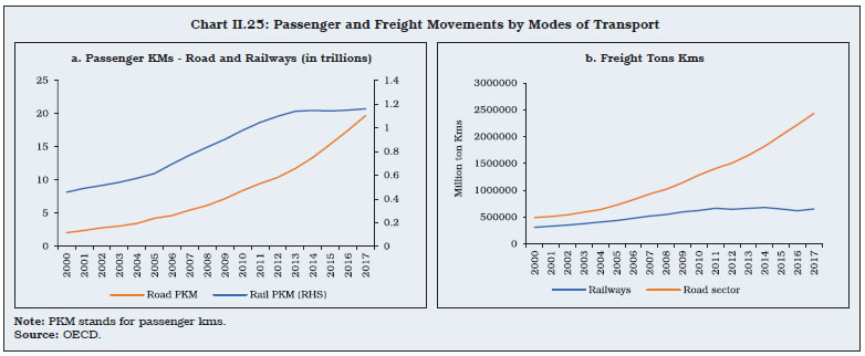 II.68 Further, mass electrification of the road transport system aided by a range of policy initiatives and technology trends, especially via the EVs, would help curtail emissions significantly. Globally, the sales of EV cars have crossed 10 million mark in 2022 with a y-o-y growth of 55 per cent. The share of EVs in total new sales is rising rapidly in India and the sales have crossed 1 million in 2022 (Chart II.26). Currently the two and three wheelers, which are mostly used for passenger transport and comprise around 76 per cent share of vehicles in India, dominate the EV sales (up to March 2023, Vahan). Moreover, 64 per cent of petrol consumption in India is by two/ three wheelers (MoPNG, 2015). In recent years, the three-wheeler e-rickshaw has become the first mile and last mile connectivity option in all the cities displacing the traditional petrol/diesel run three wheelers for short run commute. II.69 EV penetration, however, faces challenges of high upfront cost of EV vis-à-vis their internal combustion engine (ICE) counterparts and the lack of adequate EV charging infrastructure. As of April 27, 2023, India had 7010 public EV charging stations, which is low by global standards. The Government over the last ten years has undertaken a series of measures to incentivise adoption of EVs in the country, through tax incentives for EV owners and development of public EV charging infrastructure. II.70 Within the mobility sector, shipping and aviation are hard-to-abate due to the lack of cost-effective low-carbon alternatives. Bio-fuels, although expensive, is the most mature technology available today which could decarbonise aviation and shipping. Industrial Sector II.72 Decomposition analysis of industrial energy usage following Kant et al., (2022) indicates that ceteris paribus, the output effect alone would have led to a rise of 530 billion kWh in energy consumption, but the actual increase was contained at 315 billion kwh mainly because of the improvement in the energy intensity and the structural effect reflecting the shift in the composition of industries towards less energy-intensive industries (Chart II.27). Improvements in energy efficiency can be attributed to the continuous techno-economic improvements in the industries. The favourable structural effect is indicative of the rising share of less energy-intensive industries in industrial GVA. This structural effect is expected to play a much bigger role going forward as high-end manufacturing like electronics is more knowledge intensive rather than material and energy intensive. | Table II.9: Manufacturing Firms in India: Energy Intensity, Output and Emissions | | Year | Energy
(billion kWh) | CO2
(million tonnes) | GVA
(at 2011-12 prices, ₹ trillion) | Energy Intensity
(kWh per rupee GVA) | Carbon Intensity
(gram of CO2 per rupee GVA at 2011-12 prices) | | 2009-10 | 921 | 320.1 | 7.49 | 0.12 | 43.0 | | 2019-20 | 1237 | 491.8 | 12.32 | 0.10 | 39.9 | | Source: Authors’ estimates; For methodology see Kant et al., (2022). |
II.73 Overall, Indian industries largely depend on coal for their energy requirements (Table II.10). Within industry, metals, non-metallic minerals and chemicals together account for 78 per cent of the total industrial coal usage, while others primarily use electricity (Table II.11). However, a gradual shift is underway within these energy-intensive manufacturing industries, with the share of electricity rising from 12.6 per cent to 18.0 per cent during 2009-2019. | Table II.10: Share of Fuels in Indian Manufacturing Sector | | Fuel (as per cent of energy-mix) | 2009-10 | 2013-14 | 2019-20 | | Coal | 40.8 | 47.2 | 45.5 | | Gas (LPG, Biogas, Natural Gas, Coal Gas) | 17.9 | 9.3 | 11.2 | | Diesel | 3.8 | 2.6 | 5.5 | | Furnace Oil | 9.8 | 6.4 | 8.5 | | Kerosene | 0.2 | 0.4 | 0.3 | | Electricity | 16.3 | 21.5 | 22.9 | | Other (Wood, Solar, Fuel Oil) | 11.3 | 12.6 | 6.0 | | Source: Authors’ estimates. | Steel II.74 Globally, India is the second largest producer of steel with 124.4 million tons of crude steel production even though the per capita consumption at 74.7 kg is significantly lower than the world average of 229 kg (World Steel Association, 2019-20). The industry is expected to grow rapidly, with steel production increasing three-fold by 2040 (IEA, 2021). Currently, around 56 per cent of India’s steel production is based on the less polluting and less-energy intensive electric arc furnace (EAF) method as compared with the more energy-intensive and coal-dependent integrated blast furnace and basic oxygen furnace (BF/BOF). Nonetheless, with India’s demand for steel expected to rise in the coming years, there is a need to diversify towards low carbon-intensive production processes, such as harnessing VRE and its integration with EAF, in order to decarbonise steel sector. | Table II.11: Fuel Usage in Indian Manufacturing Sector (2019-20) | | Industrial Sector | Total Energy Consumption (Gwh) | Share in Total Consumption (Per cent) | | Coal | Petroleum | Gas | Electricity | Other | | Metals | 409200 | 61.8 | 9.8 | 5.1 | 20.7 | 2.5 | | Non-Metallic Minerals | 202902 | 62.0 | 8.2 | 13.8 | 12.1 | 3.9 | | Chemicals | 166697 | 33.7 | 9.5 | 29.8 | 18.4 | 8.5 | | Textiles | 83219 | 45.2 | 10.4 | 2.0 | 35.6 | 6.8 | | Food | 78085 | 23.6 | 23.0 | 5.3 | 29.3 | 18.8 | | Refinery | 49917 | 1.3 | 27.9 | 52.7 | 6.7 | 11.4 | | Paper | 45151 | 66.3 | 9.7 | 0.3 | 15.3 | 8.3 | | Electricity, Gas, Steam, AC | 30529 | 83.7 | 3.1 | 2.7 | 8.3 | 2.2 | | Electric Equipment | 29261 | 0.1 | 55.4 | 1.6 | 41.7 | 1.1 | | Rubber | 28534 | 15.9 | 22.5 | 2.4 | 54.9 | 4.3 | | Pharma | 24478 | 20.2 | 24.2 | 3.9 | 40.7 | 11.0 | | Motor Vehicles | 20002 | 0.2 | 28.5 | 16.4 | 52.9 | 2.1 | | Fabricated Metals | 12561 | 5.9 | 35.1 | 8.1 | 45.9 | 5.0 | | Machinery | 11523 | 2.8 | 34.0 | 3.4 | 53.1 | 6.8 | | Beverages | 10607 | 31.4 | 20.3 | 0.4 | 21.0 | 26.8 | | Apparel | 5890 | 7.2 | 41.1 | 1.1 | 40.1 | 10.5 | | Transport Equipment | 5539 | 0.9 | 40.4 | 6.9 | 47.7 | 4.1 | | Motor Vehicle Repair | 4604 | 0.0 | 77.8 | 5.9 | 15.5 | 0.7 | | Wood | 2909 | 16.8 | 21.0 | 0.2 | 44.9 | 17.1 | | Other | 2745 | 0.2 | 34.5 | 3.3 | 58.2 | 3.9 | | Leather | 2698 | 7.9 | 29.8 | 1.1 | 53.6 | 7.6 | | Electronics | 2292 | 0.0 | 25.5 | 1.9 | 72.2 | 0.4 | | Warehousing | 1972 | 0.0 | 40.8 | 1.6 | 56.8 | 0.7 | | Media | 1683 | 0.3 | 31.6 | 0.8 | 59.6 | 7.7 | | Tobacco | 1096 | 29.3 | 28.8 | 1.9 | 29.5 | 10.5 | | Farming | 1073 | 3.9 | 20.0 | 3.9 | 70.4 | 1.8 | | Waste Disposal | 924 | 3.6 | 34.3 | 13.2 | 30.5 | 18.5 | | Source: Authors’ estimates. | Cement II.75 India is the second largest consumer of cement globally, after China. World-wide, the cement industry is one of the major hard-to-abate industries owing to the extremely high temperature required in the kiln (around 1600 degree Celsius) and the chemical process of breaking down limestone into calcium oxide and CO2. Near-term emission reductions may be achieved through alternative cement constituents, such as calcined clays, which would reduce the clinker-to-cement ratio in blended cements. Chemical Industries Ethylene II.76 Ethylene, which is used as a raw material in the manufacture of plastics, requires oil-based feedstock for its production. In India, nearly 67 per cent of the production is naphtha-based and the rest is gas-based. There are no process emissions as the carbon gets captured in the products, even though the captured carbon is ultimately released in the atmosphere through the incineration of plastics over the lifetime of the product. Furthermore, ethylene production uses very high temperature which is difficult to electrify using current technologies. To decarbonise ethylene production, oil-based feedstock may be replaced by bio-based feedstock like bio-naptha. India’s plans to achieve a 20 per cent33 blending rate for ethanol by 2025 and further ramping up of biodiesel production could act as a catalyst as bio-naphtha is generated as a by-product in the process and could be used as a feedstock. Bulk of the biofuel production is based on the first-generation technology that converts edible biomass such as sugarcane, rice, maize for ethanol and jatropha for biodiesel which is land and water intensive. Further, upgrading production technology by switching to the second-generation bioconversion technology, which uses cellulose-based, non-edible biomass and agricultural waste, could also lead to an overall reduction in emissions. Efforts to better utilise biomass from agri-residues34 and re-cycling of plastics are effective ways to reduce emissions in this industry.35 Manufacture of Ammonia II.77 Ammonia has multiple industrial applications, however, around three-quarters of its production is primarily utilised for manufacturing fertilisers. Ammonia production, which operates at a very high temperature and is difficult to electrify, uses fossil fuel as a feedstock. While the hydrogen used in this process is currently derived from natural gas, it is possible to use renewable hydrogen as a feedstock instead. However, renewable hydrogen is more expensive to produce than hydrogen from natural gas. Going forward, as electricity prices moderate with the use of cheaper renewable sources, hydrogen sourced from electrolysis could become cheaper than natural gas. II.78 Initiatives are already underway in this direction. Greenfield investments in setting up ammonia plants at the site of wind-solar hybrid projects would ensure economic viability. For example, the Government of Rajasthan is in the process of setting up a green ammonia facility and a renewable energy power plant, which is expected to produce one million tonnes of green ammonia per annum. Also, from the demand-side, rationalising the overall use as well as using nano urea could potentially reduce the consumption of urea. Agricultural Sector II.79 Apart from being affected by climate change, agriculture itself is a major source of GHGs. Around 14 per cent of GHGs are emitted by the agriculture sector in India. The agriculture sector is the main source of CH4 and N2O emissions. CH4 emissions occur mainly due to livestock rearing (enteric fermentation and manure management) and rice cultivation. N2O is principally emitted due to the application of fertilisers to agricultural soils. Within agriculture, 54.6 per cent of GHG emissions are due to enteric fermentation, followed by 17.5 per cent from rice cultivation, 19.1 per cent from fertiliser applied to agricultural soils, 6.7 per cent from manure management, and 2.2 per cent due to field burning of agricultural residues. The CH4 emitted from enteric fermentation and rice cultivation is re-converted to CO2 in the upper atmosphere and is re-captured by plants which goes as feed to livestock. Nevertheless, due to high global warming potential of CH4, it is not considered as climate neutral in the short-run. Demand side interventions like judicious use of fertilisers can reduce N2O emissions. II.80 Further, the agriculture sector accounts for about 17 per cent of total electricity consumed along with 5.9 lakh tonnes of diesel which is mainly used in energising 20 million water pumps across the country. The dedicated agricultural feeder systems in many states could be exclusively run on renewables when the generation is high and may be switched off at low variable renewable generation period. II.81 In sum, a national sector-specific approach to green transition can succeed only if reasonable and sustained progress is achieved across all key carbon emitting sectors, which would require active participation by all stakeholders, ranging from state and local governments to private corporates and NGOs. Alongside significant technological breakthroughs required to achieve green transitioning in the hard-to-abate industrial sectors, policy focus on sectors with low emission intensity such as textiles, fisheries, land transport and services could play a complementary role by supporting India’s growth and employment objectives. India has demonstrated its capacity to achieve transformational changes in some sectors, such as renewables and agriculture (developing climate-resilient cropping patterns and seeds), and with sustained policy focus high and sustainable growth objective could be achieved notwithstanding unavoidable trade-offs in the short and medium-run. 7. Concluding Observations II.82 Research on climate change has gradually evolved to assume prominence in public policy debate. Fuelled by the changing temperature and precipitation patterns, and a rising incidence of extreme weather events globally, public awareness about the consequences of climate change has gained ground, so much so that climate policies have increasingly become target-oriented with economies aiming to achieve net zero emissions within a defined timeline. II.83 India’s diverse topography makes it vulnerable to significant risks from climate change, evidences of which are increasingly visible in rapid changes in temperature; variations in SWM rains; rising frequency and intensity of extreme weather events such as unseasonal rainfall, heatwaves, cyclones and floods. Further, the aspiration of becoming an AE by 2047 could pose a unique development challenge for India, wherein it has to balance between economic and environmental goals. In this regard, India’s climate action policy has embraced climate targets defined in terms of its NDCs, while paving a step towards achieving net zero emissions by 2070 by declaring low carbon transition pathways in key economic sectors. II.84 While the manifestation of climate change has become evident, its impact on the Indian economy could be manifold, by denting the supply potential of the economy as well as by altering demand conditions. Empirical analysis indicates that natural disasters adversely impact economic activity, i.e., lower output growth, while raising inflation. Moreover, disaster-affected regions could also witness a decline in their consumption of essential commodities owing to the diversification of funds for post-disaster reconstruction/rehabilitation needs. II.85 Further, scenario analyses to chalk out India’s transition to the net zero target by 2070, while attaining the status of an AE by 2047 suggest that India would require aggressive efforts in terms of reducing its energy intensity of output as well as improving the energy-mix as compared with the current NDC commitments. While the share of green energy in overall energy consumption has to reach to about 82 per cent from its current level of around 5.5 per cent in 2021-22, the energy intensity of output has to decline by 5.1 per cent on an annual average basis as compared with the current rate of decline of 2.3 per cent in 2021-22. In such a scenario, the implied level of energy consumption by 2070 would be 3.1 times higher as compared with the 2021-22 level. II.86 Aiming to achieve an overall macroeconomic policy balance would help provide the much-needed resilience and sustainability to the economy, given the enormous scale and wide-ranging nature of the policy measures needed for climate action. Moreover, the implications of policy actions could be widespread ranging from sector-specific imbalances in the short-run to economy-wide frictions and adjustments in the medium to long run. Empirical estimates using a standard environmental Solow-type growth model to analyse the relationship between economic growth, energy usage and emissions indicate that the economy may optimise on output and GHG emissions by having the right energy-mix – a shift to green energy from brown energy. Further, the twin objectives of becoming an AE by 2047 and achieving the net zero target by 2070 could still be possible if factors of production other than energy – labour and capital – witness productivity gains on the back of government policies and technological breakthroughs. II.87 Additionally, India’s susceptibility to physical risks emanating from climate change raises significant concerns on policy trade-offs surrounding growth-inflation. Scenario analysis indicates that the Indian economy may be deeply impacted, with inflation rising and output falling in the medium-term under a lenient mitigation plan. Risk mitigating domestic policies and global concerted efforts could, however, help in containing the adverse impact on growth and inflation. II.88 Finally, in view of the difficult policy trade-offs between containing near-term adverse output impact due to NDC commitments vis-à-vis larger output losses in the medium-run due to no policy action, a sector-specific approach to climate risk mitigation is called for. Further, since different sectors of the economy have different emission intensities, it is advisable to not have a uniform climate mitigation strategy across sectors. In this regard, alongside significant technological breakthroughs required to achieve green transitioning in the hard-to-abate industrial sectors, policy focus on sectors with low emission intensities such as textiles, fisheries, land transport and services could support India’s growth and employment objectives. India has already demonstrated its capacity to achieve major transformations in certain sectors, such as renewables and agriculture (developing climate-resilient cropping patterns and seeds). With continued policy support and focus, attaining the twin objectives of becoming an AE by 2047 and achieving the net zero emission target by 2070 may not be too ambitious, notwithstanding unavoidable trade-offs in the short and medium run. References Abatzoglou, J. T., Williams, A. P., and Barbero, R. (2019). Global emergence of anthropogenic climate change in fire weather indices. Geophysical Research Letters, 46(1), 326-336. Aggarwal, R. (2019). The impact of climate shocks on consumption and the consumption distribution in India (Doctoral dissertation, PhD Thesis, Paris School of Economics, Paris, France). Albala-Bertrand, J. M. (1993). Natural disaster situations and growth: A macroeconomic model for sudden disaster impacts. World Development, 21(9), 1417-1434. Ali, H., and Mishra, V. (2018). Increase in subdaily precipitation extremes in India under 1.5 and 2.0 C warming worlds. Geophysical Research Letters, 45(14), 6972-6982. Andersson, M., Morgan, J., and Baccianti, C. (2020). Climate change and the macro economy. ECB Occasional Paper No. 243, 1-50. Basel Committee on Banking Supervision (BCBS). (2021). Climate-Related Risk Drivers and Their Transmission Channels. British Petroleum. (2022). Energy Outlook 2022. Retrieved from: https://www.bp.com/content/dam/bp/business-sites/en/global/corporate/pdfs/energy-economics/energy-outlook/bp-energy-outlook-2022.pdf Burck, J., Uhlich, T., Bals. C., Hohne, N. and Nascimento, L. (2022). Climate Change Performance Index 2023 Background and Methodology. Germanwatch. Caballero, R., and Hammour, M. (1994). The Cleansing Effect of Recessions. American Economic Review, 84 (5), 1350-1368. Carney, M. (2016). Resolving the climate paradox. Arthur Burns Memorial Lecture, Bank of England, Berlin, 22. Central Pollution Control Board. (2020). Annual Report 2019. Chen, C., Pinar, M., and Stengos, T. (2022). Renewable energy and CO2 emissions: New evidence with the panel threshold model. Renewable Energy, 194, 117-128. Ciccarelli, M., and Marotta, F. (2021). Demand or supply? An empirical exploration of the effects of climate change on the macroeconomy. ECB Working Paper Series No. 2608, 1-59. Climate Action Tracker. (2022). Retrieved from: https://climateactiontracker.org/countries/india/ Dallmann, I., and Millock, K. (2017). Climate variability and inter-state migration in India. CESifo Economic Studies, 63(4), 560-594. Dilip, A., and Kundu, S. (2020). Climate change: macroeconomic impact and policy options for mitigating risks. RBI Bulletin, 125, 105-125. Eckstein, D., Künzel, V., and Schäfer, L. (2021). The global climate risk index 2021. Germanwatch. Euro-Mediterranean Centre on Climate Change (CMCC). (2021). G20 Climate Risk Atlas Impacts, Policy, Economics – India. Freeman, P., Keen, M., and Muthukumara, M. (2003). Dealing with Increased Risk of Natural Disasters: Challenges and Options. IMF– International Monetary Fund. Working Paper 03/197. Ghosh, S., Kundu, S., and Dilip, A. (2021). Green Swans and their Economic Impact on Indian Coastal States. Reserve Bank of India Occasional Papers, 42(1), 1-69. Ministry of Statistics and Programme Implementation, GoI. (2023). Energy Statistics India 2022. Hao, Y. (2022). Effect of economic indicators, renewable energy consumption and human development on climate change: an empirical analysis based on panel data of selected countries. Frontiers in Energy Research, 10, 841497. IMD. (2022). Annual Report. Ministry of Earth Sciences, GoI. IMD. (2019). Annual Report. Ministry of Earth Sciences, GoI. International Energy Agency (IEA). (2021). India Energy Outlook 2021. International Federation of Red Cross and Red Crescent (IFRC). (2021). India: Cyclone Amphan: Final Report. IPCC. (2018). Global Warming of 1.5°C. Cambridge University Press, USA IPCC. (2022a). Climate Change 2022: Mitigation of Climate Change. Contribution of Working Group III to the Sixth Assessment Report of the Intergovernmental Panel on Climate Change. Cambridge University Press, Cambridge University Press, Cambridge, UK and New York. IPCC. (2022b). Climate Change 2022: Impacts, Adaptation, and Vulnerability. Contribution of Working Group II to the Sixth Assessment Report of the Intergovernmental Panel on Climate Change. Cambridge University Press, Cambridge University Press, Cambridge, UK and New York. Jones, M. W., Peters, G. P., Gasser, T., Andrew, R. M., Schwingshackl, C., Gütschow, J., ... and Le Quéré, C. (2023). National contributions to climate change due to historical emissions of carbon dioxide, methane, and nitrous oxide since 1850. Scientific Data, 10(1), 155. Jones, M. W., Smith, A., Betts, R., Canadell, J. G., Prentice, I. C., and Le Quéré, C. (2020). Climate change increases the risk of wildfires. ScienceBrief Review, 116, 117. Kant, S., Kumar, M., Khan, S., and Sharma, S. (2022). Carbon Dioxide Emissions from India’s Manufacturing Sector: A Decomposition Analysis. Reserve Bank of India Occasional Papers, 43(1). Kaya, Y., and Yokobori, K. (Eds.). (1997). Environment, energy, and economy: strategies for sustainability (pp. 16-26). Tokyo: United Nations University Press. Kishore, V. and Shekhar, H. (2022). Extreme Weather Events and Vegetables Inflation in India. Economic and Political Weekly, 57 (44-45), 29. Kompas, T., Pham, V. H., and Che, T. N. (2018). The effects of climate change on GDP by country and the global economic gains from complying with the Paris climate accord. Earth’s Future, 6(8), 1153-1173. Krishnan, R., Sanjay, J., Gnanaseelan, C., Mujumdar, M., Kulkarni, A., and Chakraborty, S. (2020). Assessment of climate change over the Indian region: a report of the ministry of earth sciences (MOES), government of India (p. 226). Springer Nature. Liu, J., and Niyogi, D. (2019). Meta-analysis of urbanization impact on rainfall modification. Scientific reports, 9(1), 1-14. Loayza, N. V., Olaberria, E., Rigolini, J., and Christiaensen, L. (2012). Natural disasters and growth: Going beyond the averages. World Development, 40(7), 1317-1336. Mani, M., Bandyopadhyay, S., Chonabayashi, S., and Markandya, A. (2018). South Asia’s hotspots: The impact of temperature and precipitation changes on living standards. World Bank Publications. Masson-Delmotte, V., Zhai, P., Pörtner, H. O., Roberts, D., Skea, J., Shukla, P. R., ... and Waterfield, T. (2018). Global warming of 1.5 C. An IPCC Special Report on the impacts of global warming of, 1(5), 43-50. McKinsey Global Institute. (2020). Climate risk and response: Physical hazards and socioeconomic impacts. Ministry of Finance, GoI. (2018). Economic Survey 2017-18. Ministry of Finance, GoI. (2023). Economic Survey 2022-23. Ministry of New and Renewable Energy, GoI. (2023). Retrieved from https://mnre.gov.in/bio-energy/current-status#:~:text=As%20per%20a%20recent%20study,million%20metric%20tonnes%20per%20year. Morison, R. (2021). The Climate-Change Fight Is Adding to the Global Inflation Scare. Bloomberg (June). Murakami, H., Vecchi, G. A., and Underwood, S. (2017). Increasing frequency of extremely severe cyclonic storms over the Arabian Sea. Nature Climate Change, 7(12), 885-889. Narayanan, A., Beye, R., and Thakur, G. M. (2022). Natural Disasters and Economic Dynamics: Evidence from the Kerala Floods. Policy Research Working Papers;10084, World Bank, Washington, DC. Nandargi, S. S., & Aman, K. (2017). Computation of the standardized precipitation index (SPI) for assessing droughts over India. International Journal of Current Advanced Research, 6(12), 8545-8557. National Disaster Management Authority (NDMA). (2008). Guidelines on Management of Cyclones. National Innovations in Climate Resilient Agriculture. (2016). Annual Report 2015-16. NGFS. (2020). The macroeconomic and financial stability impacts of climate change research priorities, technical document. NGFS. (2022a). NGFS Scenarios for Central Banks and Supervisors. NGFS. (2022b). Physical Climate Risk Assessment: Practical Lessons for the Development of Climate Scenarios with Extreme Weather Events from Emerging Markets and Developing Economies: Technical Document. September 2022. 1-33. NITI Aayog. (2019). Composite water management index. Retrieved from: http://social.niti.gov.in/uploads/sample/water_index_report2.pdf. Accessed, 28, 21. Oreskes, N. (2007). The scientific consensus on climate change: How do we know we’re not wrong? Climate Change: What It Means for Us, Our Children, and Our Grandchildren, edited by Joseph F. C. DiMento and Pamela Doughman. MIT Press, 65-99. Parker, M. (2018). The impact of disasters on inflation. Economics of Disasters and Climate Change, 2(1), 21-48. Picciariello, A., Colenbrander, S., Bazaz, A., and Roy, R. (2021). The costs of climate change in India. Overseas Development Institute. Retrieved https://odi.org/en/publications/the-costs-of-climate-change-in-india-a-review-of-the-climate-related-risks-facing-india-and-their-economic-and-social-costs/. Press Information Bureau (PIB). (2015). All India Study Report to PPAC on sale of Diesel and Petrol. Ministry of Petroleum and Natural Gas, GoI. Press Information Bureau (PIB). (2022). Climate Change Performance Index. Ministry of Environment, Forest and Climate Change, GoI. Schelling, T. C. (1992). Some economics of global warming. The American Economic Review, 82(1), 1-14. Schnabel, I. (2021). Climate change and monetary policy. Finance and Development, 58(3), 53-55. Solow, R. M. (1999). Neoclassical growth theory. Handbook of macroeconomics, 1, 637-667. Somanathan, E., Somanathan, R., Sudarshan, A., and Tewari, M. (2021). The impact of temperature on productivity and labor supply: Evidence from Indian manufacturing. Journal of Political Economy, 129(6), 1797-1827. Stern, N. (2006). Stern Review: The economics of climate change. Cambridge University Press, UK. The Economic Times (2014). We’ll gain confidence in our models over time, says RBI Governor Raghuram Rajan. Retrieved from: https://economictimes.indiatimes.com/opinion/interviews/well-gain-confidence-in-our-models-over-time-says-rbi-governor-raghuram-rajan/articleshow/45355264.cms?from=mdr The Economic Times. (2022a). 742 km of metro rail lines operational in 19 cities: Par panel report. Retrieved from: https://infra.economictimes.indiatimes.com/news/urban-transportation/742-km-of-metro-rail-lines-operational-in-19-cities-par-panel-report/92992922 The Economic Times. (2022b). India plans to invest Rs 2.8 lakh crore in ISTS for RE evacuation. Retrieved from: https://energy.economictimes.indiatimes.com/news/renewable/india-plans-to-invest-rs-2-8-lakh-crore-in-ists-for-re-evacuation/95457753 United Nations Development Programme. (2022). Energy Progress Report 2022. Retrieved from https://www.undp.org/publications/energy-progress-report-2022 United Nations International Strategy for Disaster. Reduction. (2018). Economic Losses, Poverty and Disasters 1998-2017. Université Catholique de Louvain (UCL), Brussels, Belgium, 33. Volz, U. (2017). On the role of central banks in enhancing green finance. Inquiry Working Paper No. 01. World Bank. (2021). Climate Risk Country Profile: India. World Bank. (2022). Climate Investment Opportunities in India’s Cooling Sector. World Meteorological Organization. (2021). State of the Global Climate 2020. MO-No. 1264. World Meteorological Organization. World Steel Association, 2019-20. World Steel in Figures 2019. Yang, L., Tian, F., and Niyogi, D. (2015). A need to revisit hydrologic responses to urbanization by incorporating the feedback on spatial rainfall patterns. Urban Climate, 12, 128-140.
Annex II.1: The NIGEM Model – Key Features The NIGEM approach takes into account the standard NGFS scenarios as the benchmark (Annex Table 1). The deviations of various macroeconomic variables under different possible transition scenarios are then examined. The standard scenarios of NGFS are defined in terms of global GHG emissions, which are considered as the global baseline scenarios for macroeconomic impact assessment (NGFS, 2022a). | Annex Table 1: Standard NGFS Scenarios Setting the Global Benchmark | | Below 2 degree Celsius | This scenario assumes that optimal carbon prices as per the long-term path are set immediately after 2020 and keeps the 67th percentile of warming below 2 degree Celsius throughout the 21st century. | | Current Policies | Existing climate policies remain in place without any change in policy ambitions. | | Delayed Transition | This scenario assumes that the next 10 years see a ';fossil recovery” and thus, follow the trajectory of the current policy scenario until 2030. This is related to Below 2 degree Celsius scenario but follows a very skewed path due to late start. | | Divergent Net Zero | This scenario assumes that optimal carbon prices, in line with the long-term targets, are implemented immediately after 2020 after a limited temporary overshoot before reaching net zero. This is related to net zero 2050 but follows a divergent path - mitigation efforts are unevenly distributed across sectors, with stronger mitigation action taking place in the Transport and Buildings sectors-reflecting lack of coordination. | | Nationally Determined Contributions (NDCs) | This scenario foresees that currently pledged unconditional NDCs are implemented fully and respective targets on energy and emissions in 2025 and 2030 are reached in all countries. This scenario also factors in the net zero 2070 goal of India as per its NDC. | | Net Zero 2050 | This scenario foresees global CO2 emissions to be at net zero in 2050. It limits the temperature rise to 1.5 degree Celsius. Furthermore, countries with a clear commitment to a specific net-zero policy target at the end of 2020 are assumed to meet this target. |
|