Press Release RBI Working Paper Series No. 06 Liquidity Shocks and Overnight Interest Rates in Emerging Markets:
Evidence from GARCH Models for India @Bhupal Singh Abstract *This paper examines the role of key frictional and structural liquidity shocks in shaping the movement in call money rates and the pattern of volatility. Using Generalized Autoregressive Conditional Heteroscedasticity models, this study finds that both structural and frictional liquidity shocks are vital in explaining movements in call money rates in India, thus highlighting the need to deal with liquidity shocks in the transmission process. Frictional liquidity shocks are more pronounced in their impact on call money rates vis-à-vis structural liquidity shocks. The interbank call money rates in India also exhibit high persistence of volatility, which could be attributed to unanticipated accumulation of government cash balances, volatile forex inflows and spikes in currency demand. Among the instruments of liquidity management, open market operations that influence durable liquidity, emerge as a key policy instrument shaping call money rates. JEL Classification: E4, E5 Keywords: Call money interest rates, volatility, liquidity management, monetary policy Introduction The pace at which policy rates are transmitted to financial markets determines the effectiveness of monetary policy signals. The transmission of policy rate changes to financial markets is sensitive to liquidity conditions and, therefore, the impact of policy rate changes is conditioned to a large extent by the liquidity management operations of the central bank. Under the framework where the interest rate channel has emerged as the key transmission channel for central banks, managing liquidity actively to steer the target rate in the desired trajectory has become a standard operating framework. An appraisal of the liquidity demand of the banking system becomes critical for the success of liquidity management operations. For an efficient transmission of monetary policy, the central bank aims to align its overnight operating target rate close to its policy rate to guide the longer-term interest rates in the economy by way of liquidity provisions ranging from overnight window to medium-term horizon. Persistent deviation of the central bank’s target interest rate from its policy rate may trigger active liquidity absorption or injection because such deviations and consequent rise in volatility may heighten market uncertainties and make the transmission process that much weaker. Thus, liquidity management is considered to be crucial for the first leg of monetary transmission, i.e. transmission of policy rate changes to overnight money market rate. In an emerging market economy, where financial markets are not fully developed and there are numerous frictions operating in the financial system (e.g. regulated interest rates in some segments, lack of complete market integration and prevalence of sectoral credit dispensation), the efficacy of the interest rate channel of monetary policy transmission is impeded. Further, the efficacy of the transmission process to financial markets is also impeded by the prevalence of liquidity frictions, which may not be conducive for complete transmission of the policy rate changes. The operating framework of a monetary policy that has evolved across most advanced economies (AEs) and emerging market economies (EMEs) comprises mainly of an operating target interest rate of the central bank and instrument(s) to achieve the target rate. In the Indian context, the Reserve Bank of India (RBI, 2014) has suggested that liquidity management operations should be consistent with the stance of monetary policy, i.e. an increase in the policy rate to convey an anti-inflation policy should be accompanied by tightening of liquidity conditions, whereas accommodative liquidity conditions should characterise the easing of the policy standpoint. Thus, the transmission of monetary policy to interest rates at the short end of the yield curve is responsive to liquidity conditions prevailing during the policy rate change and subsequent periods. The central bank responds to various liquidity shocks in the banking system by deploying an array of liquidity management instruments. The basic operating framework of any monetary policy aims to align the weighted average call rate (WACR), i.e. the operating target, with the policy rate by proactively managing liquidity. The revised liquidity framework instituted by the Reserve Bank of India (RBI) in September 2014 aimed to make liquidity management operations flexible, transparent and predictable. Subsequently, the liquidity management framework was fine-tuned to progressively lower the average ex ante liquidity deficit to a situation closer to neutrality. The objective is to meet the requirements of durable liquidity and then use the central bank’s operations to ensure that short-term liquidity conditions are congruent with the monetary policy stance. Furthermore, the policy rate corridor around the repo rate was narrowed from +/-100 basis points to +/- 50 basis points. The prime motivation of this paper is to identify the unanticipated liquidity shocks that explain movements in call money rate and the pattern of its volatility. Thus, this paper seeks to answer the following question: How do various frictional and structural liquidity shocks shape the monetary transmission process towards the short- end and the nature of volatility in call money rates? An understanding of these issues may help improve our insight into the transmission process which faces challenges emanating from various structural constraints. Abstracting from the usual approaches to explaining money market volatility in terms of market microstructure issues, an attempt is made to identify and quantify the nature and impact of various liquidity shocks on the target interest rate of the central bank and thus offer some new insights into the transmission process. Two key questions are addressed in the paper: How important is the effect of frictional drivers vis-à-vis structural drivers in explaining the movement in overnight call money rates? How persistent is the volatility in call money rates? This study first explains the notion of frictional and structural liquidity in Section II and identifies the potential factors that cause temporary or durable demand-supply mismatches of liquidity. It also discusses a framework with a view to understand the relationship between structural and frictional liquidity and short-run target interest rates of the central bank. This is vital to understand the role liquidity shocks can play in causing changes in overnight money market rates. Section III deals with the model for empirical estimation and discusses the methodology. A variety of Generalized Autoregressive Conditional Heteroscedasticity (GARCH) models are deployed to empirically assess the impact of various factors in causing volatility and understanding the nature of volatility. The empirical estimates are reported in Section IV. Section V concludes the key findings. II. Liquidity Shocks and Money Market Volatility II.1 Theoretical Framework Banks hold liquid assets to manage any potential demand for liquidity by customers. However, banks also borrow funds from the interbank market to cover the deficiency in the supply of cash over demand, with the banks/institutions with surplus funds acting as lenders. Banks borrow and lend funds in the money market to manage liquidity and comply with regulatory obligations on reserve maintenance. The interest rate charged on such borrowings depends on the supply of funds in the market, the current interest rate environment, and the explicit stipulations of the contract such as the duration of funds borrowed. In the simple conceptual model, the role of the key drivers of bank liquidity in causing shifts in demand and supply of funds and hence determining the equilibrium price of liquidity (i.e. overnight market interest rate) are examined. The aggregate supply of liquidity is decided by the central bank and the surplus liquidity holding banks and the demand for liquidity by the banking system’s requirements for holding reserves. The objective function of the central bank with regard to liquidity management can be conceptualised as the minimisation of its loss function L(t), which involves minimisation of the squared deviations of the target variable (r) from the policy rate (r*): 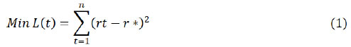 The unanticipated shocks, as alluded to in the previous section, disturb the demand-supply equilibrium in the market, which in turn leads to deviation of overnight money market interest rates from the central bank’s policy rate. In a situation where the market supply of liquidity is given, the interbank rate will be determined by the slope of the demand curve. As elucidated in Chart 1, given the liquidity supply (SL), an outward shift in liquidity demand (DL) due to factors such as currency demand, sudden changes in the government’s cash balances emanating from lumpiness in expenditure and tax flows will lead to a shift in the equilibrium position (q*) to q1 at the price (interest rate) r1. Thus, at the prevailing rate (r*), the market does not clear. The excess demand (q1-q*) in the money market creates conditions which cause the equilibrium interest rate to rise. The process will continue until a new equilibrium is reached at the point a2 where new demand for liquidity intersects the supply curve. The net result is a rise in the market price of liquidity from r* to r1 to reach a new equilibrium. It is evident from Chart 1 that when the demand for liquidity increases, the money market rate spread rises and vice versa. Thus, the marginal impact of a shift in the demand curve is  These shocks are, however, accommodated by the central bank using liquidity management operations in the form of overnight liquidity to banks, term repos and open market operations (OMOs). Nevertheless, the central bank’s supply of liquidity may not fully offset the impact of various liquidity demand shocks due to a number of factors, viz. the nature of shocks, uncertainties around the expected evolution of liquidity, distribution of liquidity among the market participants, errors in liquidity forecasts/estimation by the central bank, and rigidities created by the market microstructure. These, in turn, lead to the deviation of market rate from repo rate. Thus, after central bank intervention, the interest rate may find a new equilibrium as 
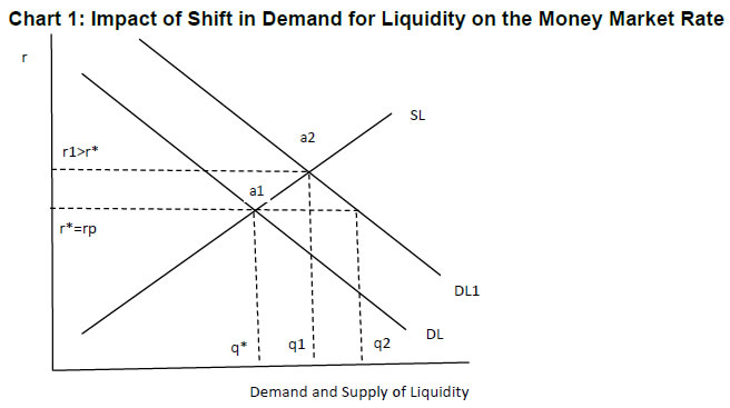 Given the demand, the effect of a shift in the supply of liquidity is elaborated in Chart 2. The demand and supply curves intersect at point a1, so r* and q* are the original equilibrium price (interest rate) and quantity of liquidity, respectively. An increase in the supply implies that a larger quantity of liquidity is offered at the same interest rate (r*) or the same amount of liquidity at a lower price. It sets in motion market forces which drive the interest rate to a new equilibrium at r2. Here again, if the central bank intervenes in the market to absorb excess liquidity, the market interest rate may settle somewhere between r* and r2. Thus, the central bank’s actions to maintain the overnight rates within its desirable corridor may lead to the following outcome, subject to various frictions and uncertainties prevailing in the market. 
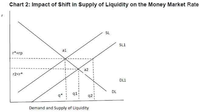 When various liquidity shocks hit the money market, the demand for reserves may be affected. The empirical literature explaining the spread between the target rate and the key policy rate of the central bank focuses on the factors which are mostly related to the market microstructure (Table 1). The central bank’s balance sheet and operational framework are found to play an important role in determining the Euro Overnight Index Average (EONIA) spread (Linzert and Schmidt, 2008).1 Some studies find that expectations of changes in the policy rate and liquidity conditions at the end of the reserve maintenance period affect the volatility of overnight rates (Wurtz, 2003). It is also documented that a spread between inter-bank and central bank policy rate is influenced by transaction costs, aggregate liquidity demand of the banking sector, costs of central bank funds, and the distribution of the latter across banks (Neyer and Wiemers, 2004). | Table 1: Market Microstructure-based Factors Impacting the Money Market | | Authors | Factors | | Moschitz (2004) | Distribution of liquidity shocks. | | Neyer and Wiemers (2004) | Heterogeneity among banks in terms of cost of funds and distribution among banks. | | Wurtz (2003), Cassola and Morana (2008) | Expectations of policy rate and liquidity conditions. | | Valimaki (2008), Linzert and Schmidt (2008) | Liquidity uncertainty. | | Cassola and Morana (2008), Beirne (2012) | Liquidity and credit risk. | | Bech and Monnet (2013) | Role of excess reserves and counterparty risk. | | Whitesell (2006) | Rate corridors; reserve requirements allow period-average smoothing of interest rates. | | Wurtz (2003) | Projected liquidity conditions at the end of the reserve maintenance period. | | Source: Author’s compilation. | In the Indian context, some research has underlined the importance of liquidity conditions in influencing monetary policy pass-through to financial markets, including the effect of policy rate changes on overnight money market rates (Ray and Prabu, 2013; Singh, 2011). Focusing specifically on the role of market microstructure on volatility in the target rate of the central bank, Ghosh and Bhattacharyya (2009) found that lag spread, besides the conditional variance of call rate, emerges as the key determinant of call money rate spread. Patra et al. (2016) assessed liquidity management by examining the performance of transmission of policy rate to the target rate of the Reserve Bank of India and the benefits thereof in terms of reducing the volatility of call money rates. Kumar et al. (2017) found that liquidity conditions, viz. deficit, distribution and uncertainty, have an adverse effect on call money rate spread. Bhattacharyya et al. (2019) underscore the significance of both rate and quantum channels in policy transmission towards the short end of the financial market. The existing empirical literature suggests that there seems to be a lack of empirical work exploring the role of underlying demand and supply shocks in explaining the movement in call money rate in India and its volatility pattern. II.2 Identification of Structural and Frictional Drivers of Liquidity in India Liquidity is determined by changes in bank reserves with the change in the underlying drivers, as exemplified in Table 2. In order to comprehend the behaviour of liquidity shocks underlying the movement in call money rates, it is important to identify various durable and transitory liquidity shocks affecting the liquidity demand. | Table 2: Central Bank Balance Sheet | | Assets | Liabilities | | Net foreign exchange reserves | Currency in circulation | | Net lending to government | Bank’s current account balances | | Lending to banks | Reserve requirements | | | Deposits | | | Capital and reserves | | Source: Central Bank websites. | Central banking functions, viz. government cash management, currency issuance and foreign exchange management, constitute the autonomous drivers of liquidity. In its role as the government’s banker, RBI’s cash management actions centre around providing liquidity to tide over the transitory deficit of the government finances, as also facilitating the deployment of surplus cash balances of the government. Further, in order to contain undue volatility in the forex market, the central bank intervenes in the market, which has implications for domestic rupee liquidity. A surge in demand for currency with the public, ceteris paribus, translates into an increase in the reserve demand of banks. Thus, banks may drawdown their surplus reserve holdings with the central bank. As explained above, the assessment of liquidity conditions necessitates an understanding of its frictional and structural drivers. The various drivers of liquidity and how they transmit to the target interest rate of the central bank are illustrated in Chart 3.  The frictional liquidity demand is regarded as transient and the drivers of such liquidity in the Indian context are identified as seasonal and festival demands for currency by the public2 and changes in the government’s cash balances with the RBI (which are in turn induced by advance tax flows and the government’s borrowing programme), which results in the demand for reserves by commercial banks.3 The structural liquidity demand is more durable in nature as the factors driving this demand are considered to be more persistent. When the wedge between deposit and credit growth of the banking system widens and persists, it assumes the character of structural liquidity demand and may force banks to meet a part of the credit demand through short-term borrowings.4 A part of the currency demand may also be driven by the underlying transaction demand in the economy consistent with income growth, which becomes more durable in nature. Liquidity demand due to persistent capital inflows and the RBI’s forex market intervention can cause more permanent changes in liquidity conditions and hence can be characterised as structural in nature.5 The best measure of the liquidity demand of the banking system is central bank liquidity because any surplus/deficit in the banking system liquidity is ultimately reflected in the liquidity adjustment facility (LAF) balances. RBI (2014) proposed a monetary policy operating framework during the transitional phase with liquidity assessment based on frictional and structural drivers. The magnitude and persistence of the impact of a shock on the call money rate may differ significantly depending on the state of liquidity in the domestic financial system. It could be possible that a frictional liquidity shock may have longer lags and higher magnitude of impact on call money rates during deficit liquidity compared with surplus liquidity conditions. The role of the LAF window is to overcome frictional liquidity deficit/ surplus, whereas the durable liquidity is to be managed with other instruments. The functional framework of the monetary policy in India comprises a single policy rate (repo rate) to indicate the monetary policy stance and operates within a corridor established by the RBI. In order to maintain its operating target (i.e. weighted average call money rate) close to its policy rate, the RBI deploys liquidity management instruments at its disposal.6 The operating objective is to contain this rate around the repo rate within the corridor. While instruments such as cash reserve ratio (CRR) and OMO are more appropriate to overcome durable or structural liquidity mismatches, overnight repo auctions are intended to tackle frictional liquidity mismatches. RBI (2019) underscored the fact that while overnight operations (or weekly/fortnightly operations followed by overnight operations) should address the liquidity needs of the banking system, unanticipated shocks could still lead to liquidity build-up that could result in actual liquidity being different from the desired level. In the case of persistent shocks, it would be essential to take the liquidity in the system back to the desired level, which could be achieved through OMOs or, where outright operations are not desirable, by deploying different tools to attain the required impact on durable liquidity. Against this backdrop, an empirical assessment of the various shocks affecting liquidity level, and hence call money rates and volatility in call rates assumes importance III. Model and Data III.1 Model It is widely believed that financial market data often display volatility clustering, i.e. sizeable changes are followed by sizeable changes and small deviations are trailed by small deviations (Mandelbrot, 1963). In fact, time-varying volatility is more common than constant volatility, and precise modelling of time-varying volatility is of major significance. In other words, while returns themselves are uncorrelated, absolute returns or their squares show a positive, significant and slowly dwindling autocorrelation function. The autoregressive conditional heteroscedastic (ARCH) (Engle, 1982) and generalised autoregressive conditional heteroscedastic (GARCH) (Bollerslev, 1986) models aim to more precisely define the phenomenon of volatility clustering and associated effects such as kurtosis, which formed the basis of the dynamic volatility models (Alexander and Lazar, 2006). The key is that volatility, rather than remaining constant or moving in a monotonic manner over time, is dependent on past realisations of the associated volatility because asset volatility tends to revert to some mean. Thus, the volatility behaviour is christened ARCH if the error variance is related to the squared error term in the previous period, and GARCH if the error variance is related to the squared error terms over several periods in the past. The ARCH model involves three distinct specifications: conditional mean equation, conditional variance, and conditional error distribution. The standard GARCH(1,1) model can be specified as:  yt is the return on asset at time t, μ is the average return, and εt is the residual return. The GARCH(1,1) models capture some of the skewness and leptokurtosis in the financial data. It allows the conditional variance to be dependent on previous own lags. The size of the parameters α and β govern the short-run dynamics of the volatility time series. If the sum of the coefficients is equal to one, a shock will lead to an enduring variation in all future values, i.e. shock is persistent. The GARCH-in-mean (GARCH-M) model is often used where the expected return on an asset is related to the expected asset risk. The estimated coefficient on the expected risk is a measure of the risk-return trade-off. A simple GARCH(1,1)-M model can be specified as  where Yt is the return of a financial asset and μ and δ are constant parameters to be estimated. δ is the risk premium. A positive δ means the return is positively related to its volatility, and vice versa. Nelson (1991) proposes the exponential GARCH (EGARCH) model that does not require non-negativity constraints. In addition, the EGARCH model allows for the asymmetric effect of news or shocks on conditional volatility. The EGARCH model in simplified form is  Threshold GARCH model was introduced independently by Zakoian (1994) and Glosten et al. (1993) wherein good news and bad news have a differential effect on variance. Thus, the variance reacts differently depending on the sign and size of the shock it receives. Taylor (1986) and Schwert (1989) proposed the standard deviation GARCH model, where instead of the variance the standard deviation is modelled. This model was generalised in Ding et al. (1993) with the Power ARCH specification. This paper uses GARCH(1,1) for modelling conditional volatility and TGARCH, EGARCH and PARCH for modelling asymmetric volatility. In order to test the presence of conditional heteroscedasticity in residuals, the Engle (1982) ARCH Lagrange multiplier (LM) test is used. The presence of the ARCH effect in itself does not invalidate the standard least square inferences; however, disregarding such effects may harm efficiency. III.2 Data The data used are of weekly frequency from the week ending June 4, 2010 to December 28, 2018.7 The post-crisis period of liquidity management is chosen, since it mostly represents the phase of deficit liquidity conditions. This period has also been characterised by important changes in the basic framework of liquidity management in India. The following variables have been used for empirical estimation: a) Repo rate of RBI (i.e. central bank’s policy rate) (REPO); b) Weighted average daily call money interest rate (r); c) Government of India’s outstanding cash balances with RBI as ratio to aggregate deposits of the banking system (GBAL_AD); d) Net foreign currency assets of RBI as ratio to aggregate deposits of the banking system (FCA_AD); e) Log of stock of currency in circulation (LCIC); f) The wedge between credit and aggregate deposit growth of the banking system in India, which captures structural liquidity mismatches (WEDGE); g) Overnight Index Swap implied 1-year rate (OIS1Y); h) RBI’s OMOs; i) Dummy variables to control for the impact of the new liquidity framework that was introduced in 2014; j) Dummy variables to control for the unusual high volatility caused by the taper tantrum across emerging markets. The data are sourced from the RBI, CEIC Data and Thomson Reuters DataStream. All the variables, except credit and deposits of the banking system, are weekly data or weekly averages based on daily data. Since the data on aggregate deposit and non-food credit are reported by the banking system on a fortnightly basis, these have been converted to weekly observations using the log-linear interpolation method. First, the test whether variables are stationary or non-stationary, is conducted using the Augmented Dickey–Fuller (ADF) test and the Phillips–Perron (PP) test. The unit root test results presented in Appendix Table A1 indicate that all the variables are stationary, except for currency demand (LCIC), forex reserves (FCA_AD) and monetary policy rate (REPO). These are transformed to stationary variables by taking the first difference. Variables are scaled using a logarithm or a common macroeconomic denominator, which keep the order of the values intact and hence results obtained through the transformation are interpretable. A dummy variable (DTaper) was also introduced to control for unusual volatility in call money rates during the period August to October 2013, signifying the period of large capital outflows from EMEs, including India, triggered by the United States Federal Reserve System’s (US Fed’s) announcement of future tapering of its policy of quantitative easing. IV. Empirical Estimates Mandelbrot (1963) obverted volatility clustering as the phenomenon whereby big changes tend to be followed by big changes, of either sign, and minor variations tend to be followed by minor variations. This phenomenon might be the result of incessant outside shocks. As illustrated in Chart 4, a phase of significant volatility in call money rate in India is now followed by a period of relatively lower volatility, and it is therefore imperative to examine the changing nature of volatility. 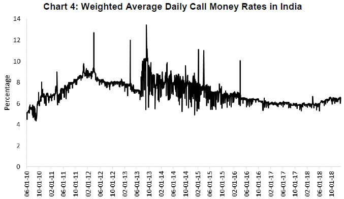 In India, the composition of RBI’s balance sheet provides some insight of the changing relative importance of various drivers of liquidity. Given the net foreign assets to gross domestic product (NFA-GDP) ratio of about 15–16 per cent of GDP, foreign exchange inflows emerge as the key driver of domestic money market liquidity in India (Chart 5). Among the durable and transitory constituents of liquidity, during the last few years, the share of LAF transactions in the total supply of liquidity, which is relatively transitory in nature, has gained greater importance vis-à-vis durable liquidity supplied through OMO operations (Chart 6). Note: Following a modification in the accounting exercise, i.e. July 11, 2014, liquidity operations (repo, term repo and Marginal Standing Facility or MSF) net of reverse repo/term reverse repo were considered as loans and advances to banks and the commercial sector instead of the earlier treatment of sale/purchase of securities. Appendix Table A2 provides the summary statistics for variables used in the GARCH models, based on weekly data spanning the sample June 2010 to December 2018. Almost all the variables had significant non-zero mean and significant positive skewness and kurtosis statistics. The Jarque–Bera statistic is significantly large, suggesting that the financial variables are not normally distributed. IV.1 Volatility Estimates from GARCH Models ARCH/GARCH models explain the heteroscedasticity of the return sequence residuals. The long memory in volatility, i.e. the effects of volatility shocks decaying slowly, occurs and is often detected by the autocorrelation in time series. There is presence of heteroscedasticity in call money rates, as the null hypothesis that there is no ARCH effect up to order q in the residuals is rejected by the LM test (Appendix Table A3). As significant changes have taken place in liquidity management and the monetary policy operational framework in India, it is apposite to test whether the parameters of the model are stable across the sample. The Quandt-Andrews unknown breakpoint test statistic suggests a sample break since April 2015 (Appendix Table A4), which reflects the period characterised by a fundamental change in RBI’s liquidity management framework that started in 2014, when the framework was changed from fixed rate repo to variable rate repo to incentivise banks to undertake active liquidity management. Based on the breakpoint test, a dummy variable (DBRK042015) is introduced for the period beginning April 2015 to consider the impact of a changed liquidity management regime. Since the diagnostic tests suggest the presence of the ARCH effect in the model, it is apposite to estimate the GARCH models. The conditional variance of the weighted average call money rate for the period June 2010 to December 2018, using weekly data, is presented in Chart 7. The volatility in the call money rate is followed by a pattern of clustering, i.e. periods of high volatility followed by periods of low volatility. Lower conditional variance after 2015 could be attributed to the revised liquidity management framework aimed at reducing the volatility in the overnight operating target rate. The large spike in volatility in 2015 was caused by uncertainties over Greece debt crisis and the deflating stock market bubble in China that engendered capital flight to safe haven. Conditional variance of the estimated GARCH model is presented in Chart 7. 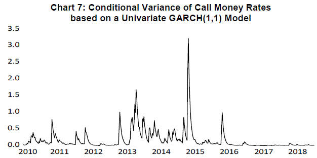 In general, the GARCH(1,1) model captures volatility clustering in the data using the maximum likelihood estimator. The LM test suggests that the model is free from ARCH effects. A diagnostic test was performed in the form of the Ljung–Box Q-test to test the null hypothesis of no serial correlation in errors. Q-statistics for the standardised residuals (Q1) and for their squared values (Q2) are computed, especially testing for the tenth lag, inspired by Tse (1998). Q2-statistics were not significant at the 5 per cent level, implying no rejection of the null hypothesis of no serial correlation in the error term. The GARCH(M) model indicates a significant positive effect of the taper tantrum on call money rates in India. The dummy variable captures the structural break caused by the new liquidity management framework. The autoregressive coefficient of the lagged dependent variables for mean equations is statistically significant and high, which implies that call money rates are significantly influenced by past lags. For GARCH(M), TARCH and IGARCH models, ARCH parameter in Table 3 is α and GARCH parameter is β. In conditional variance equations, the estimated β coefficients are considerably greater than α, which implies that the market has a memory longer than one period and that volatility is more sensitive to its lagged values than it is to new surprises in the market. (α + β)>1, indicating that the volatility shocks are quite persistent—often observed in high frequency financial data. In the EGARCH specification, γ is the asymmetry parameter, measuring the leverage effect, α is size parameter, measuring the magnitude of shocks, and persistency is captured through β. The coefficients γ, the asymmetry and leverage effects, are statistically insignificant at the 5 per cent level in both the augmented EGARCH and PARCH models. In view of the signs and statistical insignificance of γ in the EGARCH and PARCH models, the hypothesis of asymmetry and leverage effect is rejected.8 Thus, negative shocks have no different effect on the conditional variance when compared to positive shocks. The persistence parameter, β, is large and significant, underscoring the role of the persistence of past volatility in explaining the current volatility in call money rates. | Table 3: Results of GARCH(1,1) Model 1 for Weighted Average Call Money Rates | | Coefficients | GARCH(M) | TGARCH | IGARCH | EGARCH | PARCH | | Mean Equation | | | | | | | Ω | 0.63 | 0.62 | 1.05 | 0.63 | 0.66 | | | (6.91) | (7.25) | (9.45) | (5.57) | (7.14) | | r(-1) | 0.92*** | 0.92*** | 0.88*** | 0.92*** | 0.92*** | | | (82.53) | (79.86) | (62.20) | (63.44) | (75.90) | | DTaper | 0.41*** | 0.46*** | 0.37*** | 0.36*** | 0.37*** | | | (2.64) | (2.70) | (5.41) | (3.10) | (2.97) | | DBRK042015 | -0.13*** | -0.12*** | -0.29*** | -0.14*** | -0.15*** | | | (-5.02) | (-5.63) | (-10.42) | (-4.73) | (-6.51) | | Variance Equation | | | | | | | ω | 0.00*** | 0.00*** | | -0.42*** | 0.01*** | | | (4.98) | (5.09) | | (-9.78) | (6.30) | | α | 0.47*** | 0.49*** | 0.08*** | 0.45*** | 0.29*** | | | (7.33) | (8.63) | (19.02) | (8.95) | (9.53) | | β | 0.69*** | 0.68*** | 0.92*** | 0.95*** | 0.78*** | | | (26.27) | (31.34) | (220.36) | (135.34) | (43.04) | | α+β | 1.16 | 1.17 | 1.00 | 1.40 | 1.07 | | ϒ | | -0.14 | | 0.03 | -0.12 | | | | (-1.18) | | (0.81) | (-1.38) | | Log likelihood | -29.80 | -28.71 | -46.74 | -18.41 | -17.40 | | ARCH LM test statistics | 0.00 | 0.02 | 15.16 | 0.86 | 2.07 | | Prob. Chi-square (1) | (0.96) | (0.88) | (0.23) | (0.35) | (0.15) | | L-B(10), RES | 59.29 | 59.24 | 74.88 | 62.45 | 64.32 | | | (0.00) | (0.00) | (0.00) | (0.00) | (0.00) | | L-B(10), SQR RES | 5.12 | 5.22 | 14.69 | 5.92 | 7.57 | | | (0.88) | (0.88) | (0.14) | (0.82) | (0.67) | | R2 | 0.90 | 0.89 | 0.90 | 0.90 | 0.89 | | DW | 2.64 | 2.62 | 2.50 | 2.62 | 2.60 | | N | 447 | 447 | 447 | 447 | 447 | Note: ***, ** and * denote significance at 1%, 5% and 10% levels.
Z-values (in parentheses), Ljung–Box Q-statistics of the tenth lag of residuals and squared residuals are reported.
ARMA terms are used to estimate the mean, while GARCH terms are used to estimate the variance. | The results of the various specifications of the GARCH models are presented in Table 4, with mean equations augmented for a number of liquidity demand and supply shocks affecting call money rates. It needs to be emphasised that misspecification of the mean equation could fail to address the autocorrelation problem that could arise in the volatility model. Therefore, all the GARCH family models are estimated using different specifications of the mean equation, considering key liquidity demand shocks, market expectations of interest rates, durable liquidity infusion by the central bank and the changes in policy rates, all affecting the call money rates. The estimated mean equations across the family of estimated GARCH models reveal that accumulation of government cash balances with the central bank puts significant upward pressure on call money rates as the overnight liquidity is drained out of the banking system. A rise in the demand for currency also works as an escape of liquidity from the system and exerts an upward pressure on call money rates. In India, the role of currency demand in influencing liquidity conditions and hence influencing call money rates is of vital importance given that the currency-GDP ratio is around 11 per cent. The build-up of foreign currency balances of the central bank through market interventions leads to the infusion of domestic liquidity, which is found to have a moderating impact on overnight money rates. The forex inflow shocks are generally in the nature of a sudden spurt in portfolio inflows or outflows, led by risk-on and risk-off behaviour of foreign investors, which is a common phenomenon observed across EMEs. The dummy variable for the taper tantrum episode (DTaper), which led to large capital outflows from EMEs, resulted in significant tightening of call money rates. The dummy for the structural break since April 2015, indicating the impact of the new liquidity management framework, is also found to have significantly impacted call money rates. The estimates from GARCH(M) and TGARCH models reveal that the sum of the ARCH and GARCH coefficients (α+β) is greater than1, signifying that volatility shocks are fairly persistent, as is evident from financial market data. While the asymmetric effect of positive/negative news on volatility in interest rates is absent, there is evidence of high persistence of past volatility. | Table 4: Results of GARCH(1,1) Model 2 for Weighted Average Call Money Rates | | Coefficients | GARCH(M) | TGARCH | IGARCH | EGARCH | PARCH | | Mean Equation | | | | | | | Ω | 0.58 | 0.57 | 1.01 | 0.63 | 0.75 | | | (6.13) | (6.19) | (8.59) | (5.43) | (6.50) | | GBAL_AD | 0.01* | 0.01* | 0.02** | 0.02** | 0.02** | | | (1.78) | (1.71) | (2.63) | (2.08) | (2.04) | | DLCIC | 0.50*** | 0.50*** | 0.32* | 0.37** | 0.41*** | | | (3.47) | (3.46) | (1.77) | (2.31) | (2.62) | | DFCA_AD | -0.06** | -0.06** | -0.11*** | -0.04 | -0.05** | | | (-2.20) | (-2.20) | (-4.79) | (-1.58) | (-1.91) | | DTaper | 0.41*** | 0.39*** | 0.39*** | 0.36*** | 0.38*** | | | (2.63) | (2.62) | (5.72) | (3.03) | (3.04) | | DBRK042015 | -0.12*** | -0.12*** | -0.26*** | -0.14*** | -0.18*** | | | (-4.94) | (-5.13) | (-8.89) | (-4.96) | (-6.32) | | r(-1) | 0.92*** | 0.92*** | 0.88*** | 0.92*** | 0.90*** | | | (73.06) | (76.86) | (59.51) | (62.98) | (61.14) | | Variance Equation | | | | | | | Ω | 0.00*** | 0.00*** | | -0.47*** | 0.01*** | | | (3.22) | (3.29) | | (-9.27) | (4.04) | | α | 0.48*** | 0.48*** | 0.09*** | 0.51*** | 0.32*** | | | (6.86) | (8.36) | (13.54) | (7.98) | (8.56) | | β | 0.68*** | 0.68*** | 0.91*** | 0.95*** | 0.76*** | | | (28.60) | (30.58) | (139.33) | (102.54) | (35.36) | | α+β | 1.16 | 1.16 | 1.00 | 1.46 | 1.08 | | ϒ | 0.01 | | | 0.00 | -0.03 | | | (0.05) | | | (0.09) | (-0.41) | | Log likelihood | -25.71 | -25.83a3 | -41.21 | -15.46 | -14.21 | | ARCH LM test statistics | 0.02 | 0.03 | 19.17 | 0.81 | 2.05 | | p-value | (0.88) | (0.86) | (0.09) | (0.37) | (0.15) | | L-B(10), RES | 60.61 | 60.54 | 70.75 | 61.83 | 64.76 | | p-value | (0.00) | (0.00) | (0.00) | (0.00) | (0.00) | | L-B(10), SQR RES | 6.01 | 5.89 | 18.35 | 6.22 | 7.76 | | p-value | (0.81) | (0.83) | (0.11) | (0.80) | (0.65) | | R2 | 0.90 | 0.89 | 0.90 | 0.89 | 0.89 | | DW | 2.62 | 2.62 | 2.47 | 0.90 | 2.59 | | N | 447 | 447 | 447 | 447 | 447 | Note: ***, ** and * denote significance at 1%, 5% and 10% levels.
Z-values (in parentheses); Ljung–Box Q-statistics of the 10th lag of residuals and squared residuals are reported.
ARMA terms are used to estimate the mean, while GARCH terms are used to estimate the variance. | The model is estimated by including some additional variables in the mean equation to understand the role of liquidity shocks on call money rates (Table 5). A key driver of liquidity demand in money markets is the wedge between the credit and deposit growth of the banking system (i.e. a measure of durable liquidity demand-supply mismatch). A higher wedge between the credit and deposit growth signals durable liquidity mismatches in the banking system. Given the supply of bank reserves, a higher wedge therefore causes persistent excess demand for liquidity in the banking system, which tends to exert upward pressure on call money rates. It is observed that apart from the usual drivers of liquidity (i.e. government cash balances, currency demand and forex reserve inflows), the structural variable, measured as the wedge between the credit and deposit growth of the banking system (WEDGE), plays an important role in explicating the movement in call money rates. The variance equation explains that the sum of ARCH and GARCH parameters is greater than one, implying high persistence of volatility. While there is no evidence of any significant asymmetric effect of good or bad news on interest rate volatility, the past volatility is found to have significant influence on current volatility in overnight interest rates. | Table 5: Results of GARCH(1,1) Model 3 for Weighted Average Call Money Rates | | Coefficients | GARCH(M) | GARCH/TARCH | IGARCH | EGARCH | PARCH | | Mean Equation | | | | | | | Ω | 0.56 | 0.56 | 0.90 | 0.66 | 0.75 | | | (6.31) | (6.38) | (7.28) | (5.30) | (6.27) | | GBAL_AD | 0.01 | 0.01 | 0.02** | 0.02 | 0.02** | | | (1.48) | (1.48) | (2.13) | (1.57) | (1.97) | | DLCIC | 0.52*** | 0.52*** | 0.38*** | 0.43*** | 0.58*** | | | (3.22) | (3.26) | (2.44) | (2.45) | (3.20) | | DFCA_AD | -0.04* | -0.04* | -0.12*** | -0.05** | -0.05** | | | (-1.75) | (-1.79) | (-5.21) | (-1.88) | (-2.02) | | WEDGE | 0.02* | 0.02* | 0.43*** | 0.15 | 0.01 | | | (1.76) | (1.77) | (3.14) | (1.13) | (1.50) | | DTaper | 0.39** | 0.37** | 0.37*** | 0.37*** | 0.37*** | | | (2.29) | (2.29) | (5.55) | (3.13) | (2.95) | | DBRK042015 | -0.10*** | -0.10*** | -0.24*** | -0.15*** | -0.17*** | | | -(4.68) | (-4.79) | (-7.79) | (-4.75) | (-6.03) | | r(-1) | 0.93*** | 0.93*** | 0.89*** | 0.91*** | 0.90*** | | | (82.03) | (82.43) | (58.11) | (57.47) | (58.60) | | Variance Equation | | | | | | | Ω | 0.00 | 0.00 | | -0.46 | 0.01 | | | (2.84) | (2.79) | | (-9.12) | (3.42) | | α | 0.54*** | 0.54*** | 0.09*** | 0.51*** | 0.33*** | | | (7.33) | (9.18) | (14.70) | (8.19) | (8.43) | | β | 0.67*** | 0.67*** | 0.91*** | 0.96*** | 0.76*** | | | (26.48) | (32.56) | (148.75) | (102.83) | (32.24) | | α+β | 1.20 | 1.21 | 1.00 | 1.47 | 1.09 | | ϒ | | 0.04 | | 0.00 | -0.02 | | | | (0.75) | | (-0.09) | (-0.26) | | Log likelihood | -23.44 | -23.53 | -38.26 | -14.46 | -12.85 | | ARCH LM test statistics | 0.00 | 0.00 | 15.50 | 0.81 | 1.94 | | Prob. Chi-square (1) | (0.98) | (0.97) | (0.10) | (0.37) | 0.16 | | L-B(10), RES | 59.74 | 59.70 | 67.45 | 60.62 | 64.56 | | | (0.00) | (0.00) | (0.00) | (0.00) | 0 | | L-B(10), SQR RES | 6.48 | 6.33 | 16.11 | 6.18 | 7.73 | | | (0.77) | (0.79) | (0.10) | (0.80) | (0.56) | | R2 | 0.90 | 0.90 | 0.90 | 0.89 | 0.90 | | DW | 2.63 | 2.62 | 2.49 | 2.59 | 2.58 | | N | 447 | 447 | 447 | 447 | 447 | Note: ***, ** and * denote significance at 1%, 5% and 10% levels.
Z-values (in parentheses), Ljung–Box Q-statistics of the tenth lag of residuals and squared residuals are reported.
ARMA terms are used to estimate the mean, while GARCH terms are used to estimate the variance. | In Table 6, the GARCH model is augmented by introducing changes in the central bank’s policy rates. Policy rate variations emerge as the most important determinant of call money rates, as is evident from the mean equation. Again, the sum of ARCH and GARCH effect parameters is greater than one, suggesting high persistence of volatility. In the EGARCH equation, the ARCH parameter is denoted by α, which measures the reaction of conditional volatility to market shocks, suggesting that the effect of size is significant in influencing call money rate volatility. The impact of past volatility on current interest rate volatility, β, continues to be overwhelming. | Table 6: Results of GARCH(1,1) Model 4 for Weighted Average Call Money Rates | | Coefficients | GARCH(M) | GARCH/TARCH | IGARCH | EGARCH | PARCH | | Mean Equation | | | | | | | Ω | 0.44 | 0.44 | 0.90 | 0.96 | 0.60 | | | (5.68) | (5.73) | (6.98) | (5.92) | (6.93) | | GBAL_AD | 0.01* | 0.01* | 0.02** | 0.01 | 0.01 | | | (1.70) | (1.71) | (2.19) | (0.10) | (0.54) | | DLCIC | 0.83*** | 0.83*** | 0.34** | 0.40*** | 0.66*** | | | (6.45) | (6.46) | (2.00) | (2.53) | (4.43) | | DFCA_AD | -0.06** | -0.06** | -0.11*** | -0.05 | -0.04** | | | -(2.33) | (-2.34) | (-4.44) | (-1.55) | (-1.89) | | DREPO | 0.59*** | 0.59*** | 0.41*** | 0.50*** | 0.54*** | | | (6.60) | (6.65) | (3.24) | (4.28) | (6.21) | | DTaper | 0.36** | 0.35** | 0.39*** | 0.42*** | 0.38*** | | | (1.96) | (1.96) | (5.76) | (3.63) | (2.73) | | DBRK042015 | -0.07*** | -0.08*** | -0.25*** | -0.20*** | -0.12*** | | | -(3.61) | (-3.71) | (-7.59) | (-5.17) | (-6.52) | | r(-1) | 0.94*** | 0.94*** | 0.89*** | 0.87*** | 0.92*** | | | (92.69) | (93.03) | (56.14) | (42.04) | (80.98) | | Variance Equation | | | | | | | Ω | 0.00 | 0.00 | | -0.39 | 0.01 | | | (1.88) | (1.84) | | (-8.42) | (2.66) | | α | 0.61*** | 0.61*** | 0.09*** | 0.44*** | 0.33*** | | | (8.41) | (9.33) | (14.66) | (7.50) | (8.22) | | β | 0.64*** | 0.64*** | 0.91*** | 0.96*** | 0.76*** | | | (28.89) | (31.84) | (148.22) | (119.65) | (36.75) | | α+β | 1.26 | 1.26 | 1.00 | 1.40 | 1.09 | | ϒ | | 0.05 | | 0.03 | -0.12 | | | | (0.73) | | (0.84) | (-1.40) | | Log likelihood | -16.57 | -16.63 | -37.22 | -12.11 | -4.71 | | ARCH LM test statistics | 0.01 | 0.01 | 15.04 | 0.60 | 1.27 | | Prob. Chi-square (1) | (0.91) | (0.93) | (0.13) | (0.44) | (0.21) | | L-B(10), RES | 60.76 | 60.56 | 70.27 | 59.84 | 62.49 | | | (0.00) | (0.00) | (0.00) | (0.00) | (0.00) | | L-B(10), SQR RES | 6.94 | 6.78 | 14.67 | 5.24 | 7.16 | | | (0.73) | (0.75) | (0.14) | (0.88) | (0.71) | | R2 | 0.90 | 0.89 | 0.90 | 0.89 | 0.89 | | DW | 2.64 | 2.64 | 2.51 | 2.49 | 2.50 | | N | 447 | 447 | 447 | 447 | 447 | Note: ***, ** and * denote significance at 1%, 5% and 10% levels.
Z-values (in parentheses), Ljung-Box Q-statistics of the 10th lag of residuals & squared residuals are reported.
ARMA terms are used to estimate the mean, while GARCH terms are used to estimate the variance. | The mean equations are further augmented by including the one-year Overnight Index Swap implied 1-year rate (OIS1Y), which captures the market expectations on future interest rates. There is evidence of future interest rate expectations playing a critical part in influencing call money rates, as is evident from Table 7. Endurance of volatility is manifested as the sum of α and β exceeds unity. In the IGARCH, EGARCH and PARCH models, the estimated β parameter is considerably greater than α, which indicates that volatility is more responsive to its lag values than it is to new shocks. γ, the leverage coefficient, is negative but not statistically significant, exhibiting the absence of a leverage effect in the call money market, which implies that negative shocks do not generate more volatility in call money rates in India compared to the positive shocks. | Table 7: Results of GARCH(1,1) Model 5 for Weighted Average Call Money Rates | | Coefficients | GARCH(M) | GARCH/TARCH | IGARCH | EGARCH | PARCH | | Mean Equation | | | | | | | Ω | 0.21 | 0.22 | 0.59 | 0.06 | 0.28 | | | (1.94) | (2.03) | (4.64) | (1.18) | (2.30) | | GBAL_AD | 0.04*** | 0.04*** | 0.04*** | 0.02*** | 0.03*** | | | (4.89) | (5.32) | (4.50) | (2.81) | (3.31) | | DLCIC | 0.52*** | 0.46** | 0.14 | -0.11 | 0.51*** | | | (3.03) | (2.70) | (0.90) | (-0.43) | (2.61) | | DFCA_AD | -0.01 | -0.01 | -0.11*** | 0.01 | -0.03 | | | (-0.31) | (-0.28) | (-4.55) | (0.09) | (-1.17) | | OIS1Y | 0.15*** | 0.15*** | 0.15*** | 0.26*** | 0.14*** | | | (6.45) | (6.75) | (7.37) | (18.53) | (6.27) | | DTaper | 0.43*** | 0.39*** | 0.34*** | 0.18** | 0.32*** | | | (3.53) | (3.28) | (5.77) | (2.10) | (3.37) | | DBRK042015 | -0.12*** | -0.11*** | -0.25*** | -0.16*** | -0.14*** | | | (-5.75) | (-5.88) | (-8.75) | (-10.56) | (-6.07) | | r(-1) | 0.82*** | 0.83*** | 0.78*** | 0.74*** | 0.83*** | | | (45.99) | (51.07) | (40.92) | (68.59) | (47.62) | | Variance Equation | | | | | | | Ω | 0.00 | 0.00 | | -0.51 | 0.01 | | | (2.30) | (2.15) | | (-5.17) | (4.54) | | α | 0.71*** | 0.76*** | 0.10*** | 0.49*** | 0.43*** | | | (7.50) | (10.33) | (13.01) | (5.51) | (8.88) | | β | 0.59*** | 0.57*** | 0.90*** | 0.94*** | 0.70*** | | | (20.19) | (27.14) | (117.49) | (43.22) | (24.04) | | α+β | 1.30 | 1.33 | 1.00 | 1.46 | 1.13 | | ϒ | | -0.13 | | -0.09* | -0.04 | | | | (-0.45) | | (-1.75) | (-0.54) | | Log likelihood | -2.81 | -3.88 | -25.36 | 48.45 | 7.04 | | ARCH LM test statistics | 0.06 | 0.06 | 12.08 | 0.32 | 0.36 | | Prob. Chi-square (1) | (0.81) | (0.81) | (0.28) | (0.57) | (0.55) | | L-B(10), RES | 61.59 | 62.07 | 77.23 | 65.18 | 68.05 | | | (0.00) | (0.00) | (0.00) | (0.00) | (0.00) | | L-B(10), SQR RES | 6.44 | 5.72 | 11.90 | 4.01 | 4.82 | | | (0.76) | (0.84) | (0.29) | (0.94) | (0.90) | | R2 | 0.91 | 0.90 | 0.90 | 0.90 | 0.90 | | DW | 2.59 | 2.55 | 2.36 | 2.55 | 2.54 | | N | 447 | 447 | 447 | 447 | 447 | Note: ***, ** and * denote significance at 1%, 5% and 10% levels.
Z-values (in parentheses), Ljung-–Box Q-statistics of the tenth lag of residuals and squared residuals are reported.
ARMA terms are used to estimate the mean, while GARCH terms are used to estimate the variance. | The mean equations of GARCH models in Table 8 capture the effect of OMOs of the central bank in influencing call money rates. It is well understood that durable infusion (or absorption) of liquidity into the money market through outright purchases (or sale) of securities can significantly influence the movement in call money rates on a durable basis. The mean equations reveal that OMOs (OMO_AD) emerge as the most dominant variable explaining movement in call money rates. The variance equation reveals that volatility in the money market tends to be persistent. The estimated β coefficient in the TARCH, IGARCH and PARCH models is considerably greater than α, implying that rather than market surprises, volatility is more responsive to its lags, which indicates that volatility is more sensitive to its lagged values than to surprises in the market. Some evidence of a significant leverage effect in the money market is present, implying that negative news influences volatility more than the positive news, though the effect is moderate. Such negative shocks could emanate from certain factors, viz., news of sudden changes in risk-taking behaviour of foreign portfolio investors, unexpected pressures in currency markets, global market developments, etc. Second, the impact of past volatility on current interest rate volatility continues to be strong and persistent. | Table 8: Results of GARCH(1,1) Model 6 for Weighted Average Call Money Rates | | Coefficients | GARCH(M) | TARCH | IGARCH | EGARCH | PARCH | | Mean Equation | | | | | | | Ω | 0.86 | 2.04 | 2.25 | 0.91 | 2.26 | | | (7.66) | (7.91) | (11.39) | (6.34) | (8.64) | | GBAL_AD | 0.03*** | 0.00 | 0.00 | 0.03*** | -0.01 | | | (3.55) | (-0.11) | (0.58) | (3.84) | (-0.58) | | DLCIC | 0.88*** | 0.23 | 0.20 | 0.59*** | 0.15 | | | (4.45) | (1.48) | (1.31) | (3.30) | (0.32) | | DFCA_AD | -0.02 | -0.07** | -0.07** | -0.01 | -0.06** | | | -(0.65) | (-2.05) | (-2.33) | (-0.21) | (-1.99) | | OMO_AD | -0.32** | -0.56*** | -0.83*** | -0.49*** | -0.66*** | | | -(2.28) | (-3.48) | (-6.78) | (-3.50) | (-4.07) | | DTaper | 0.10 | 0.57*** | 0.52*** | 0.68*** | 0.48*** | | | (1.06) | (5.44) | (6.19) | (7.86) | (3.73) | | DBRK042015 | -0.29*** | -0.49*** | -0.57*** | -0.29*** | -0.55*** | | | -(11.84) | (-8.09) | (-11.94) | (-8.28) | (-8.89) | | r(-1) | 0.91*** | 0.74*** | 0.72*** | 0.90*** | 0.71*** | | | (58.28) | (22.64) | (28.86) | (46.98) | (21.59) | | Variance Equation | | | | | | | Ω | 0.00 | 0.00 | | -1.64 | 0.01 | | | (3.38) | (1.67) | | (-13.11) | (1.58) | | α | 1.56*** | 0.17*** | 0.11*** | 1.30*** | 0.20*** | | | (7.45) | (4.34) | (10.27) | (11.79) | (5.59) | | β | 0.20*** | 0.84*** | 0.89*** | 0.60*** | 0.85*** | | | (4.70) | (28.01) | (82.06) | (21.30) | (36.91) | | α+β | 1.76 | 1.01 | 1.00 | 1.90 | 1.05 | | ϒ | | 0.07 | | -0.27** | 0.13 | | | | (1.48) | | (-2.60) | (1.66) | | Log likelihood | 5.07 | 9.66 | 2.33 | 15.09 | 14.95 | | ARCH LM test statistics | 0.08 | 0.42 | 2.46 | 0.12 | 3.29 | | Prob. Chi-square (1) | (0.76) | (0.52) | (0.12) | (0.72) | (0.19) | | L-B(10), RES | 32.69 | 37.73 | 50.68 | 36.64 | 47.26 | | | (0.00) | (0.00) | (0.00) | (0.00) | (0.00) | | L-B(10), SQR RES | 7.86 | 4.95 | 5.75 | 10.40 | 7.20 | | | (0.64) | (0.89) | (0.84) | (0.41) | (0.71) | | R2 | 0.87 | 0.88 | 0.88 | 0.85 | 0.88 | | DW | 2.69 | 2.43 | 2.40 | 2.57 | 2.42 | | N | 447 | 447 | 447 | 447 | 447 | Note: ***, ** and * denote significance at 1%, 5% and 10% levels.
Z-values (in parentheses), Ljung-–Box Q-statistics of the tenth lag of residuals and squared residuals are reported.
ARMA terms are used to estimate the mean, while GARCH terms are used to estimate the variance. | V. Conclusion The primary aim of this paper is to examine the effect of structural and frictional liquidity shocks on call money rates and the pattern of volatility. The results from a family of estimated GARCH models suggest the following. Among the key exogenous liquidity shocks impacting call money rates in India, there is strong evidence of currency demand, forex inflows and movements in government’s cash balances with the RBI as principal drivers. While tax revenues are predictable, expenditures are lumpy, causing unanticipated liquidity demand/supply and hence higher volatility in the movement of call money rates. Given the significant currency-GDP ratio in India, movements in currency demand result in sudden changes in money market liquidity, which in turn impacts call money rates. Forex inflows, particularly led by portfolio inflows, are more volatile in nature as these are strongly influenced by foreign investors’ expectations and risk-taking behaviour. A key structural driver of liquidity demand in money markets is the wedge between the credit and deposit growth of the banking system. There is also a compelling evidence of this variable influencing the movement in call money rates. Future expectations of interest rates are also found to significantly influence call money rates. Among the key components of central bank operations—while changes in central bank policy rate (i.e. repo rate) strongly influence the call money rates in India—OMO sales/purchases, which absorb/inject durable liquidity in the money market, emerge as a key policy instrument influencing the call money rate. OMO purchases by the central bank from the banking system lead to the injection of durable liquidity in the financial system, resulting in a strong moderating impact on money market rates. The paper estimates the nature of volatility of call money rates in India using the symmetric and asymmetric GARCH models. The conditional variance based on various GARCH models suggests that there has been a moderation in volatility in call money rates since 2015, which could be the outcome of the introduction of a new liquidity framework. The evidence of the persistence of volatility in call money rates could be attributed to the presence of various frictional drivers of liquidity. There is strong evidence of past volatility causing current volatility in call money rates. The asymmetric outcome seized by the estimated EGARCH and PARCH models shows that there does not seem to be clear evidence of negative shocks to the money market causing more volatility than positive shocks. The results from the mean equation models underscore the importance of frictional and structural drivers in influencing movements in call money rates, which have vital significance from the viewpoint of a liquidity management policy. The results also emphasise the role of durable liquidity operations of the central bank in strongly influencing call money rates.
References Alexander, C., & Lazar, E. (2006). Normal mixture GARCH(1,1): Applications to foreign exchange markets. Journal of Applied Econometrics, 21(2), 307–336. Bech, M., & Monnet, C. (2013). The impact of unconventional monetary policy on the overnight interbank market. Reserve Bank of Australia Conference. In A. Heath, M. Lilley & M. Manning (Eds.), Liquidity and Funding Markets, Proceedings of a Conference, Reserve Bank of Australia, Sydney. Beirne, J. (2012). The EONIA spread before and during the crisis of 2007–2009: The role of liquidity and credit risk. Journal of International Money and Finance, 31(3), 534–551. Bhattacharyya, I., Behera, S. R., & Talwar, B. (2019). Contours of liquidity management: Developments during 2018–19. RBI Bulletin, LXXIII(2), February. Bollerslev, T. (1986). Generalized autoregressive conditional heteroskedasticity. Journal of Econometrics, 31(3), 307–27. Cassola, N., & Morana, C. (2008). Modelling short-term interest rate spreads in the euro money market. Working Paper Series No. 982, European Central Bank. Ding, Z., Granger, C. W. J., & Engle, R. F. (1993). A long memory property of stock market returns and a new model. Journal of Empirical Finance, 1, 83–106. Engle, R. F. (1982). Autoregressive conditional heteroskedasticity with estimates of the variance of United Kingdom inflation. Econometrica, 50(4), 987–1007. Ghosh, S., & Bhattacharyya, I. (2009). Spread, volatility and monetary policy: Empirical evidence from the Indian overnight money market. Macroeconomics and Finance in Emerging Market Economies, 2(2), 257–277. Glosten, L. R., Jaganathan, R., & Runkle, D. (1993). On the relation between the expected value and the volatility of the normal excess return on stocks. Journal of Finance, 48, 1779–1801. Kumar, S., Prakash, A., & Kushawaha, K. M. (2017). What explains call money rate spread in India? RBI Working Paper Series: 07/2017. Linzert, T., & Schmidt, S. (2008). What explains the spread between the euro overnight rate and the ECB’s policy rate? Working Paper Series No. 983/December, European Central Bank. Mandelbrot, B. B. (1963). The variation of certain speculative prices. Journal of Business, 36, 392–417. Moschitz, J. (2004). The determinants of the overnight interest rate in the euro area. Working Paper Series No. 393/September, European Central Bank. Nelson, D. B. (1991). Conditional heteroskedasticity in asset returns: A new approach, Econometrica, 59, 347–370. Neyer, U., & Wiemers, J. (2004). The influence of a heterogeneous banking sector on the interbank market rate in the euro area. Swiss Journal of Economics and Statistics, 140, 395–428. Patra, M. D., Kapur, M., Kavediya, R., & Lokare, S. M. (2016). Liquidity management and monetary policy: From corridor play to marksmanship, Pages 257-296. In C. Ghate and K. M. Kletzer (Eds.), Monetary policy in India: A modern macroeconomic perspective, Springer, New Delhi, India. Ray, P., & Prabu, E. (2013). Financial development and monetary policy transmission across financial markets: What do daily data tell for India? RBI Working Paper Series, 04/2013. Reserve Bank of India (RBI) (2011a). Third Quarter Review of Monetary Policy 2010–11, January. — (2011b). Report of the Working Group on Operating Procedure of Monetary Policy, March. — (2012). Annual Report 2011-12, Reserve Bank of India, August. — (2014). Report of the Expert Committee to Revise and Strengthen Monetary Policy Framework, January. — (2019). Report of the Internal Working Group to Review the Liquidity Management Framework, September. Singh, B. (2011). How asymmetric is the monetary policy transmission to financial markets in India? Reserve Bank of India Occasional Papers, 32(2), 1–37. Schwert, W. (1989). Stock volatility and crash of ’87. Review of Financial Studies, 3, 77–102. Taylor, S. (1986). Modeling financial time series. New York: John Wiley & Sons. Tse, Y. K. (1998). The conditional heteroscedasticity of the yen–dollar exchange rate. Journal of Applied Econometrics, 13(1), 49–55. Valimaki, T. (2008). Why the effective price for money exceeds the policy rate in the ECB tenders? Working Paper Series No. 981, European Central Bank. Whitesell, W. (2006). Interest rate corridors and reserves. Journal of Monetary Economics, 53, 1177–1195. Wurtz, F. R. (2003). A comprehensive model of the euro overnight rate. Working Paper Series No. 207, European Central Bank. Zakoian, J. M. (1994). Threshold heteroskedastic models. Journal of Economic Dynamics and Control, 18, 931–944.
Appendix | Table A1: Unit Root Tests | | Variable | Augmented Dickey–Fuller | Test Critical Value at 5% | Phillips-Perron Test Statistic | Test Critical Value at 5% | | R | -3.45* | -3.42 | -4.42* | -3.42 | | GBAL_AD | -5.75* | -3.42 | -5.49* | -3.42 | | FCA_AD | -3.12 | -3.42 | -2.81 | -3.42 | | DFCA_AD | -16.13* | -2.87 | -19.09* | -2.87 | | LCIC | -1.32 | -2.87 | -3.12 | -3.42 | | DLCIC | -7.45* | -2.87 | -10.32* | -2.87 | | WEDGE | -2.25* | -1.94 | -2.13* | -1.94 | | REPO | -2.07 | -2.87 | -2.07 | -2.87 | | DREPO | -3.24* | -2.87 | -21.10* | -2.87 | | OIS1Y | -3.74* | -3.42 | -3.89* | -3.42 | | OMO_AD | -2.96* | -2.87 | -16.24* | -2.87 | | *: Significant at 5% level. |
| Table A2: Summary Statistics | | | WEDGE | r | REPO | OMO_AD | OIS1Y | LCIC | GBAL_AD | FCA_AD | | Mean | 1.00 | 7.10 | 7.08 | -0.01 | 7.32 | 9.49 | 0.56 | 22.83 | | Median | 0.77 | 6.98 | 7.25 | 0.00 | 7.43 | 9.50 | 0.50 | 22.74 | | Maximum | 7.78 | 10.84 | 8.50 | 0.18 | 9.78 | 9.92 | 3.12 | 26.03 | | Minimum | -9.87 | 4.64 | 5.25 | -0.18 | 5.00 | 9.05 | -0.93 | 20.37 | | Std. Dev. | 3.43 | 1.05 | 0.85 | 0.05 | 0.83 | 0.24 | 0.72 | 1.15 | | Skewness | -0.66 | 0.39 | 0.01 | -1.04 | 0.13 | -0.04 | 0.43 | 0.51 | | Kurtosis | 3.87 | 2.74 | 1.68 | 6.07 | 2.56 | 1.97 | 2.92 | 2.84 | | Jarque– Bera | 46.81 | 12.53 | 32.65 | 184.31 | 5.01 | 19.97 | 14.19 | 19.68 | | | (0.00) | (0.00) | (0.00) | (0.00) | (0.08) | (0.00) | (0.00) | (0.00) | | Observations | 448 | 448 | 448 | 321* | 448 | 448 | 448 | 448 | Note: * Smaller number of observations for OMO_AD is due to availability of weekly data since June 2014.
Figures in parenthesis are p-values, indicating significance level. |
| Table A3: Heteroscedasticity Test: ARCH | | Variables | F-statistic | Engle’s LM Test Statistic
(Obs*R-squared) | | r | 57.22 | 50.92 | | (0.00) | (0.00) | | Note: Figures in parenthesis are p-values, indicating significance level. |
| Table A4: Quandt-Andrews Unknown Breakpoint Test Statistic for r | | | Maximum LR F-statistic | Maximum Wald F-statistic | | Breakpoint date 10/4/2015 | 14.21 | 28.42 | | (0.00) | (0.00) | | Note: Figures in parenthesis are p-values, indicating significance level. | |