| I. Macroeconomic Outlook Inflation is expected to firm up during the first quarter of 2018-19 before moderating in the remaining part of 2018-19 as the direct impact of the increase in house rent allowances for central government employees fades away, which has to be looked through. Economic activity is expected to accelerate with the strengthening of investment activity, supported by consumption demand and robust credit growth. The Monetary Policy Report (MPR) of October 2017 flagged significant shifts underway in the macroeconomic environment. Some of them have gained traction since then while others are incipiently in motion. Global economic activity has continued to strengthen and is becoming increasingly synchronised across regions. Global trade is outpacing demand after lagging behind for two years. Oil prices have firmed up again on the edge of a delicate demand-supply balance. Generally buoyant global financial markets have been interrupted by bouts of volatility triggered by several event-specific announcement effects, and most recently by reassessments of the pace of monetary policy normalisation in the US. Renewed fears of protectionism, retaliatory actions and trade wars pose a major challenge to the global economy, with implications for emerging market economies (EMEs), including India, that are participating in open international trade and relying on foreign capital flows to realise their developmental aspirations. After languishing for five consecutive quarters, economic activity in India is quickening, as estimates and high frequency as well as survey-based indicators etch out for the second half of 2017-18. Growth is strengthening and several elements are coming together to nurture this nascent acceleration: expectations of a record foodgrains output; strong sales growth by corporations; depleting finished goods inventories; and, restart of investment in fixed assets by corporations pointing to renewal of the capex cycle. Several services sectors, including the information technology sector in terms of its international competitiveness, have shown resilience. These are some of the developments that support brighter prospects for the Indian economy in 2018-19. A significant development has been that this time around, the step-up in growth is propelled by a revival of investment on the demand side and manufacturing on the supply side. This outlook will be lifted by tailwinds from remonetisation and implementation of Goods and Services Tax (GST). The path of inflation will likely be influenced by effects of the increase in house rent allowances (HRAs) for central government employees, which is purely statistical and has to be looked through to gauge true inflation developments. As this effect wanes, inflation could moderate in the remaining part of 2018-19 from an upturn in Q1 under the baseline assumptions. Fiscal slippages for 2017-18 and 2018-19, along with the postponement of the medium-term adjustment path, are a key risk to the growth and inflation outlook. Monetary Policy Committee: October 2017-February 2018 The Monetary Policy Committee (MPC) met in December 2017 and February 2018 in accordance with the pre-announced bi-monthly schedule. The MPC voted to keep the policy rate on hold in these meetings, maintaining its neutral stance of the fourth bi-monthly resolution of October 2017. The MPC’s resolutions as well as individual minutes and voting patterns reflected concerns about the changing inflation trajectory – upside risks to the inflation outlook from food and fuel prices, rising input cost conditions, fiscal slippages, and volatile global financial markets in its December resolution; and increase in HRAs by state governments, crude oil and other commodity prices, revisions to minimum support prices (MSPs) and fiscal slippages in its February resolution. The seasonal moderation in prices of vegetables and fruits, subdued capacity utilisation, and moderate rural real wage growth were seen as mitigating factors. | Table I.1 Monetary Policy Committees and Voting Patterns | | Country | Number of Policy Meetings: October 2017-March 2018 | | Total Meetings | Meetings With Full Consensus | Meetings With Dissents | | Brazil | 4 | 4 | 0 | | Chile | 5 | 5 | 0 | | Colombia | 5 | 1 | 4 | | Czech Republic | 4 | 3 | 1 | | Hungary | 5 | 5 | 0 | | Israel | 4 | 3 | 1 | | Japan | 4 | 0 | 4 | | South Africa | 3 | 1 | 2 | | Sweden | 3 | 2 | 1 | | Thailand | 4 | 3 | 1 | | UK | 4 | 2 | 2 | | US | 4 | 3 | 1 | | Source: Central bank websites. | Against this backdrop, the MPC voted in December by a majority of 5-1 to maintain status quo on the policy rate, while continuing with a neutral stance. As in the October meeting, one member voted for a rate cut to support economic activity. In February, the MPC persevered with status quo on the policy rate with a vote of 5-1 and a neutral stance, while reiterating its commitment to keep headline inflation close to 4 per cent on a durable basis. In view of several drivers of inflation firing at the same time and the upper tolerance band of inflation target under threat, one member voted for a 25 basis points (bps) increase in the policy rate to commence the withdrawal of accommodation. These subtle variations in voting patterns reflecting individual members’ views on the current and evolving macroeconomic outlook as well as policy preferences on the weights they assign to deviations of inflation and output from target/ potential are also observed in recent experiences of the MPCs in other countries (Table I.1). Macroeconomic Outlook Chapters II and III present macroeconomic developments during October 2017–March 2018 and also explain the reasons for deviations of actual outcomes of inflation and growth from staff’s projections in the October 2017 MPR. Turning to the outlook, the recent evolution of domestic and global macroeconomic developments warrant revisions in the baseline assumptions (Table I.2). | Table I.2: Baseline Assumptions for Near-Term Projections | | Indicator | October 2017 MPR | Current (April 2018) MPR | | Crude Oil (Indian Basket) | US$ 55 per barrel during 2017-18: H2 | US$ 68 per barrel during 2018-19 | | Exchange rate | ₹ 65/US$ | Current level | | Monsoon | 5 per cent below LPA in 2017 | Normal for 2018 | | Global growth | 3.5 per cent in 2017
3.6 per cent in 2018 | 3.9 per cent in 2018
3.9 per cent in 2019 | | Fiscal deficit | To remain within BE 2017-18
(3.2 per cent of GDP) | To remain within BE 2018-19
(3.3 per cent of GDP) | | Domestic macroeconomic/ structural policies during the forecast period | No major change | No major change | Notes: 1. The Indian basket of crude oil represents a derived numeraire comprising sour grade (Oman and Dubai average) and sweet grade (Brent) crude oil processed in Indian refineries in the ratio of 72:28.
2. The exchange rate path assumed here is for the purpose of generating staff’s baseline growth and inflation projections and does not indicate any ‘view’ on the level of the exchange rate. The Reserve Bank is guided by the objective of containing excess volatility in the foreign exchange market and not by any specific level of/band around the exchange rate.
3. Global growth projections are from the World Economic Outlook (July 2017 and January 2018 updates), International Monetary Fund (IMF).
4. BE: Budget Estimates.
5. LPA: Long period average (average rainfall during 1951-2000). | First, crude oil prices (Indian basket) firmed up from US$ 56 a barrel in October 2017 to US$ 67 a barrel in January 2018 (Chart I.1). Thereafter, they have fluctuated between US$ 60 and US$ 67. With the Organisation of the Petroleum Exporting Countries (OPEC) extending production cuts through the end of 2018 and the drawdown of inventories to meet increasing demand, being buffeted somewhat by the response of US shale oil production, the baseline scenario assumes crude oil prices (Indian basket) to average around US$ 68 a barrel in 2018-19. Second, the exchange rate (Indian rupee vis-à-vis the US dollar) has exhibited two-way movements since October 2017. It appreciated till the early part of January 2018 on buoyant capital inflows and weakening of the US dollar. Subsequently, it depreciated from early February, following the release of stronger than expected US non-farm payrolls and wages data that fuelled expectations of a faster pace of interest rate increases by the US Federal Reserve and over concerns of the impact of higher crude oil prices on India’s trade deficit. By March, the exchange rate of the rupee was close to its October 2017 level. 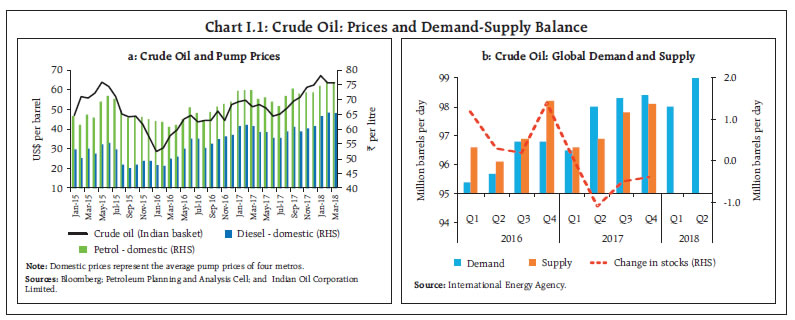 Third, the pace of global economic activity in 2017 turned out to be stronger than expected due to robust growth in the advanced economies (AEs) and significantly stronger growth in EMEs. Global growth is expected to accelerate further in 2018, benefitting from the boost to investment demand in the US from corporate tax cuts, robust recovery in the euro area and generally improved growth outlook in EMEs (Chart I.2). The sharp recovery in world trade is expected to sustain in 2018 and enlarge the prospects of another year of strong and resilient global activity. I.1 The Outlook for Inflation Headline CPI inflation reached a peak of 5.2 per cent in December 2017 (4.9 per cent, excluding the estimated impact of HRA for central government employees), reflecting an unseasonal spike in the prices of vegetables and the full impact of the central government implementing the 7th Central Pay Commission’s (CPC’s) HRA award. The delayed setting in of the seasonal food prices moderation took down headline inflation to 4.4 per cent in February (4.1 per cent, excluding the estimated impact of HRA for central government employees). It is likely that this softening will keep the reading for March benign before it reverses in April. The incidence and strength of this reversal will condition monetary policy responses in 2018-19. Turning to the outlook, inflation expectations of urban households remain elevated, according to the March 2018 round of the Reserve Bank’s survey.1 Inflation expectations three months ahead and a year ahead increased by 30 bps and 10 bps, respectively, from the previous round (December) to 7.8 per cent and 8.6 per cent, respectively. The proportion of respondents expecting the general price level to increase by more than the current rate declined for both three months and one year horizons (Chart I.3). 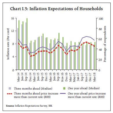 Manufacturing firms polled in the Reserve Bank’s industrial outlook survey (March 2018) expected higher input price pressures in Q1:2018-19 due to rising cost of raw materials (higher negative values for cost of raw materials indicate higher input price pressures) (Chart I.4).2 Selling prices are also expected to increase, but not sufficient to protect profit margins. The Nikkei’s purchasing managers’ survey also indicates both input and output price pressures for manufacturing (March 2018) as well as services (February 2018) sectors. Professional forecasters surveyed by the Reserve Bank in March 2018 expect CPI inflation to firm up to 5.1 per cent in Q1:2018-19 and moderate thereafter to 4.3 per cent in Q4:2018-19 (Chart I.5).3 Their medium-term inflation expectations (5 years ahead) remained unchanged at 4.5 per cent, while longer-term inflation expectations (10 years ahead) increased by 40 bps to 4.5 per cent. 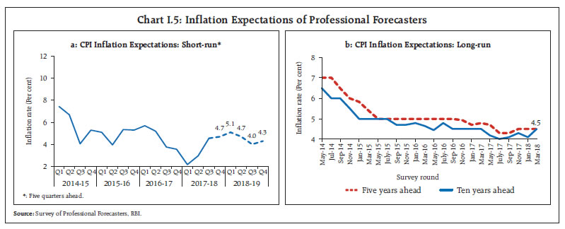 Taking into account the initial conditions, signals from the forward looking surveys and estimates from structural and other models, CPI inflation is projected to pick up from 4.4 per cent in February 2018 to 5.1 per cent in Q1:2018-19 due to unfavourable base effects and then moderate to 4.7 per cent in Q2, and 4.4 per cent in Q3 and Q4, with risks tilted to the upside (Chart I.6). It may be noted that the direct impact of the increase in the HRA announced by the Central Government fades away fully by December 2018. The 50 per cent and the 70 per cent confidence intervals for inflation in Q4:2018-19 are 3.2-5.9 per cent and 2.5-6.7 per cent, respectively. Excluding the estimated impact of HRA for central government employees, CPI inflation would pick up from 4.1 per cent in February 2018 to 4.7 per cent in Q1:2018-19 and then moderate to 4.4 per cent in Q2, Q3 and Q4. For 2019-20, assuming a normal monsoon and no major exogenous/policy shocks, structural model estimates indicate that inflation will move in a range of 4.5-4.6 per cent. The 50 per cent and the 70 per cent confidence intervals for Q4:2019-20 are 3.0-6.1 per cent and 2.2-7.0 per cent, respectively. There are a number of upside risks to the baseline forecasts. Although the direct impact on headline inflation is statistical and should be looked through for policy purposes, second order effects of the expected increases in HRA, including by state governments, can impact inflation expectations. Other major risks to the inflation outlook are crude oil and other commodity prices, the proposed revisions to MSPs for kharif crops, and fiscal slippage at both the central and state levels. I.2 The Outlook for Growth Going forward, economic activity is expected to gather pace in 2018-19, benefitting from a conducive domestic and global environment. First, the teething troubles relating to implementation of the GST are receding. Second, credit off-take has improved in the recent period and is becoming increasingly broad-based, which portends well for the manufacturing sector and new investment activity. Third, large resource mobilisation from the primary market could strengthen investment activity further in the period ahead. Fourth, the process of recapitalisation of public sector banks and resolution of distressed assets under the Insolvency and Bankruptcy Code (IBC) may improve the business and investment environment. Fifth, global trade growth has accelerated, which should encourage exports and reduce the drag from net exports. Sixth, the thrust on rural and infrastructure sectors in the Union Budget could rejuvenate rural demand and also crowd in private investment. Notwithstanding these salubrious developments, consumer confidence dipped in the March 2018 round of the Reserve Bank’s survey, with the respondents expecting a moderation over the year ahead in general economic conditions, employment situation and their income (Chart I.7).4 Overall sentiment in the manufacturing sector a quarter ahead also fell in the March 2018 round of the Reserve Bank’s industrial outlook survey under the weight of weaker prospects for production, order books, capacity utilisation, employment and profit margins (Chart I.8). However, surveys conducted by other agencies indicate an improvement in business confidence (Table I.3). Manufacturing and services sector firms in the Nikkei’s purchasing managers’ surveys (March 2018 and February 2018, respectively) are optimistic about the outlook a year ahead, driven by expansion plans and expected improvement in demand conditions. | Table I.3: Business Expectations Surveys | | Item | NCAER Business Confidence Index
(January 2018) | FICCI Overall Business Confidence Index
(February 2018) | Dun and Bradstreet Composite Business Optimism Index
(January 2018) | CII Business Confidence Index (December 2017) | | Current level of the index | 129.3 | 71.6 | 91.0 | 59.7 | | Index as per previous Survey | 118.5 | 65.6 | 76.7 | 58.3 | | % change (q-o-q) sequential | 9.1 | 9.1 | 18.6 | 2.4 | | % change (y-o-y) | 15.4 | 23.0 | 39.1 | 5.7 | Notes: 1. NCAER: National Council of Applied Economic Research.
2. FICCI: Federation of Indian Chambers of Commerce & Industry.
3. CII: Confederation of Indian Industry. |
In the March 2018 round of the Reserve Bank’s survey, professional forecasters expected real gross domestic product (GDP) growth to pick up marginally from 7.2 per cent in Q3:2017-18 to 7.3 per cent in Q1:2018-19 and remain at 7.2 per cent in Q2-Q4 (Chart I.9 and Table I.4). Taking into account the baseline assumptions, survey indicators and model forecasts, real GDP growth is projected to improve from 6.6 per cent in 2017-18 to 7.4 per cent in 2018-19 – 7.3 per cent in Q1, 7.4 per cent in Q2, 7.3 per cent in Q3 and 7.6 per cent in Q4 – with risks evenly balanced around this baseline path.5 For 2019-20, the structural model estimates indicate real GDP growth at 7.7 per cent, with quarterly growth rates in the range of 7.4-7.9 per cent, assuming a normal monsoon, and no major exogenous/policy shocks (Chart I.10). 
| Table I.4: Reserve Bank’s Baseline and Professional Forecasters’ Median Projections | | (Per cent) | | | 2017-18 | 2018-19 | 2019-20 | | Reserve Bank’s Baseline Projections | | | | | Inflation, Q4 (y-o-y) | 4.5 | 4.4 | 4.5 | | Inflation excluding the estimated impact of HRA for central government employees, Q4 (y-o-y) | 4.2 | 4.4 | 4.5 | | Real GDP Growth | 6.6 | 7.4 | 7.7 | | Assessment of Survey of Professional Forecasters@ | | | | | Inflation, Q4 (y-o-y) | 4.7 | 4.3 | | | Real GDP Growth | 6.6 | 7.3 | | | Gross Domestic Saving (per cent of GNDI) | 30.2 | 30.5 | | | Gross Fixed Capital Formation (per cent of GDP) | 28.5 | 29.0 | | | Credit Growth of Scheduled Commercial Banks | 10.0 | 11.3 | | | Combined Gross Fiscal Deficit (per cent of GDP) | 6.5 | 6.3 | | | Central Government Gross Fiscal Deficit (per cent of GDP) | 3.5 | 3.3 | | | Repo Rate (end-period) | 6.00 | 6.00 | | | Yield of 91-days Treasury Bills (end-period) | 6.2 | 6.3 | | | Yield of 10-years Central Government Securities (end-period) | 7.6 | 7.5 | | | Overall Balance of Payments (US$ billion) | 27.1 | 11.3 | | | Merchandise Exports Growth | 9.0 | 9.4 | | | Merchandise Imports Growth | 18.0 | 10.9 | | | Current Account Balance (per cent of GDP) | -1.9 | -2.1 | | @: Median forecasts; GNDI: Gross National Disposable Income.
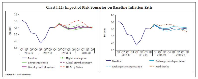
Source: RBI staff estimates; and Survey of Professional Forecasters (March 2018). | Risks to the baseline growth scenario need to be monitored carefully. First, the uncertainty associated with the pace and timing of normalisation of monetary policy in the US and other major AE central banks has led to recurrent bouts of volatility in international financial markets which may have an adverse impact on capital flows and overall investment sentiment, including for EMEs through the “finance” channel. Second, protectionist measures in the US and the generalised threat of a trade war can exacerbate volatility in global financial markets, with spillovers to domestic financial markets and adverse implications for the growth outlook. Large revisions in past data on national accounts statistics also pose a challenge to forecasts (Box I.1). I.3 Balance of Risks The baseline projections of growth and inflation presented in the preceding sections are based on assumptions set out in Table I.2. However, there are large uncertainties around these baseline assumptions, posing risks to the baseline projections. The projected paths of growth and inflation under plausible alternative scenarios are discussed below. (i) International Crude Oil Prices The dynamics of oil prices over the past six months highlight the volatility associated with the oil market. The baseline scenario assumes crude oil prices (Indian basket) to average around US$ 68 a barrel during 2018-19. Global growth has surprised on the upside in recent quarters. If these conditions persist, global crude oil demand and hence prices could edge higher. Assuming crude oil prices average around US$ 78 in this scenario, inflation could be higher by 30 bps over the baseline and growth weaker by around 10 bps. On the other hand, there could be downward pressures on international crude prices if global economic activity were to turn weaker than expected (for a variety of factors discussed later) or shale gas output is ramped up further in response to elevated crude oil prices or OPEC members produce more than their agreed shares. Should the Indian basket crude price fall to US$ 58 per barrel in this scenario, inflation could ease by around 30 bps below the baseline, with a boost of around 10 bps to real GDP growth (Charts I.11 and I.12). Box I.1: National Accounts Data Revisions in India With the advancement of first advance estimates (FAE) of national accounts data by the Central Statistics Office (CSO) to the first week of January, the issue of large revisions in data has come to the fore. The first advance estimates are based on limited information, which get addressed gradually in successive revisions. An analysis of revisions of annual growth rates of major components of GDP in India between the first release and the latest available release shows a generally upward bias. On the production side, an analysis based on annual data (2003-04 onwards) and quarterly data (2002-03 onwards) reveals that the CSO revised annual real gross value added (GVA) growth estimates relative to advance estimates upwards in ten years (on an average of about 70 basis points), and downwards in the remaining four years (on an average of about 27 basis points) (Table I.1.1). In the case of real GDP, advance estimates were revised up in twelve years (an average of 81 basis points), and revised downwards only in two years (an average of 204 basis points). An analysis of GVA components shows that significant revisions were mainly in three sectors, viz. ‘mining and quarrying’, ‘manufacturing’ and ‘financial, real estate and professional services’. | Table I.1.1: First and Last Estimates of Real GVA Growth: Mean and Median of Differences (in percentage points) | | Variable | Annual Growth Rate (14 years) | Quarterly Growth Rate (60 quarters) | | Mean | Median | Mean | Median | | GVA | 0.43 | 0.37 | 0.55 *** | 0.54 *** | | Agriculture, forestry and fishing | 0.84 | 0.99 | 0.34 | 0.74 * | | Mining and quarrying | 2.34 | 1.18 | 1.97 *** | 0.58 *** | | Manufacturing | 2.06 | 1.75 | 2.09 *** | 1.13 *** | | Electricity, gas, water supply and other utility services | -0.20 | -0.36 | 0.35 | 0.45 * | | Construction | 1.34 | 0.51 | 0.75 | 0.60 | | Trade, hotels, transport, communication and services related to broadcasting | 0.47 | 0.87 | 0.34 | 0.64 | | Financial, real estate and professional services | 0.49 | 0.43 | 1.08 *** | 1.23 *** | | Public administration, defence and other services | -1.31 | -0.81 | -0.46 | -1.10 | Notes: 1. ***, ** and * indicates statistical significance at 1%, 5% and 10%, respectively.
2. Wilcoxon sign rank test has been performed for median.
3. The null hypothesis is that there is no difference in parameters for two or more sets of population. | From the expenditure side, the analysis of annual data from 2007-08 onwards and for quarterly data from 2009-10 onwards shows that private final consumption expenditure (PFCE), and exports and imports of goods and services were revised significantly (Table I.1.2). The analysis also reveals that during periods of rising growth, initial estimates were revised upwards in successive revisions, while during the periods of slackening of growth, revisions were in the downward direction – initial estimates understate in magnitude both upswings and downswings. Advance estimates of GDP/GVA growth may, therefore, need to be supplemented with high frequency indicators to arrive at a realistic assessment of the state of the economy (Prakash et al, 2018). Reference: Prakash, Anupam, A. K. Shukla, A. P. Ekka and K. Priyadarshi (2018), “Examining Gross Domestic Product Data Revisions in India”, Mint Street Memo (forthcoming), Reserve Bank of India. | Table I.1.2: First and Last Estimates of Real GDP Growth-Expenditure Side: Mean and Median of Differences (in percentage points) | | Variable | Annual Growth Rate (10 years) | Quarterly Growth Rate (32 quarters) | | Mean | Median | Mean | Median | | GDP | 0.38 | 0.56 | 0.71** | 0.36** | | Private final consumption expenditure | 1.56 | 1.14 | 1.31** | 1.19** | | Government final consumption expenditure | -0.92 | 0.41 | -0.12 | 2.49 | | Gross fixed capital formation | 1.96 | 1.91 | 2.89* | 0.80 | | Exports of goods and services | 1.97 | 1.29 | 3.59* | 2.04* | | Imports of goods and services | 2.99 | 2.43 | 15.33 | 2.67** | | Notes: Please see notes to Table I.1.1. | |
 (ii) Global Growth The baseline scenario assumes global growth to gain upward momentum during 2018, buoyed by the boost to US investment demand from corporate tax cuts, strong activity in the euro area supported by accommodative monetary policy and improvement in growth prospects of EMEs. There are upside risks to the baseline with the synchronised cyclical rebound, revival of global trade and easy financing conditions reinforcing each other. If global growth turns out to be 50 bps over the baseline, it could strengthen domestic growth by 20 bps above the baseline and raise domestic inflation by around 10 bps. 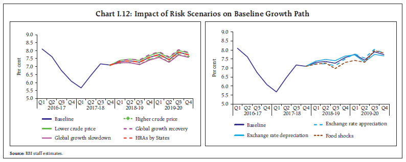 On the other hand, protectionist policies, continuing uncertainty associated with the pace and timing of normalisation of monetary policy in the US and other systemic central banks, and higher crude oil prices pose downside risks to global demand. In such a scenario, if global demand weakens by 50 bps vis-à-vis the baseline, domestic growth and inflation could be 20 bps and around 10 bps, respectively, below the baseline. (iii) House Rent Allowances – Implementation by States The increase in the HRA by the central government for its employees is reflected in the inflation data since July 2017. There remains uncertainty, however, about the magnitude and timing of implementation of the HRA award by the state governments for their employees and these are, therefore, not included in the baseline inflation path. Assuming that all state governments implement increases in pay and allowances of the same order as the central government during the course of 2018-19, CPI inflation could turn out to be around 100 bps above the baseline on account of the direct statistical effect of higher HRAs, with additional indirect effects emanating from higher demand and increase in inflation expectations. As noted earlier, monetary policy should look through the direct statistical effects, while being vigilant about indirect effects working through inflation expectations. (iv) Exchange Rate The exchange rate of the Indian rupee vis-à-vis the US dollar has moved in both directions in recent months. Changing market perceptions about the pace and timing of monetary policy normalisation in the US, along with domestic inflation, fiscal slippage and current account balance developments, have been important factors driving exchange rate movements in the recent period and are likely to remain so in the near-term. With economic activity gathering pace in the euro area, uncertainty surrounding normalisation plans of the European Central Bank is likely to add to financial market volatility. The US macroeconomic policy mix – easy fiscal policy in an environment when monetary accommodation is being withdrawn – can accentuate market volatility. Assuming a depreciation of the Indian rupee by around 5 per cent relative to the baseline, inflation could edge higher by around 20 bps and the boost to net exports could increase growth by around 15 bps. On the other hand, with growth picking up in recent months, sound domestic fundamentals and the various initiatives taken by the Government to boost investment, India may continue to be an attractive destination for foreign investment, which could put upward pressures on the currency. An appreciation of the Indian rupee by 5 per cent in this scenario could soften inflation by around 20 bps and reduce growth by around 15 bps in 2018-19. (v) Risks to Food Inflation The baseline projections of growth and inflation assume a normal south-west monsoon, which is supported by early signals of likely ENSO (El Nino – Southern Oscillation) neutral conditions. The India Meteorological Department (IMD) is yet to release its forecast on the south-west monsoon season for 2018. Given the sensitivity of the agricultural sector to rainfall conditions, the actual growth and inflation dynamics would critically depend on the progress of the monsoon. A deficient monsoon could lower overall GDP growth by around 20-30 bps in 2018-19. Furthermore, the Union Budget has proposed revised guidelines for arriving at the MSPs for kharif crops, although the details are not yet fully available. If the monsoon is deficient and the budget proposals on MSPs lead to higher food prices, headline inflation could rise above the baseline by around 80 bps. (vi) Fiscal Slippage The Central Government’s fiscal deficit for 2017-18 and 2018-19 is likely to be above initial expectations and the medium-term adjustment path has also been postponed. An empirical assessment presented in the MPR of October 2017 suggests that: (a) in India, causality runs from fiscal deficits to inflation; and (b) the impact of fiscal deficits on inflation is non-linear, i.e., higher the initial levels of the fiscal deficit and inflation, higher is the impact of an increase in the fiscal deficit on inflation. Given the present levels of the combined (centre and states) fiscal deficit, an increase in the fiscal deficit to GDP ratio by 100 bps could lead to an increase of about 50 bps in inflation. Apart from its direct impact on inflation, fiscal slippage has broader macro-financial implications, notably on economy-wide costs of borrowing which have already started to rise. These may feed into inflation and elevate it further. I.4 Conclusion To summarise, aggregate demand is expected to improve in 2018-19, supported, inter alia, by the improving GST implementation, the recapitalisation of public sector banks and the resolution of distressed assets under the IBC. Rural and infrastructure sectors are identified as thrust areas in the Union Budget, which could energise aggregate demand. With the acceleration in global trade, the Indian economy could benefit from buoyant external demand. In addition to the usual monsoon related uncertainty, inflation faces upside risks from a variety of other sources, especially due to the oil prices, the fiscal slippage, and (the statistical effect from) the expected increases in HRAs by the state governments, The purely direct statistical impact of the HRA adjustment on CPI will be looked through while formulating monetary policy. Uncertainty over the pace and timing of monetary policy normalisation by the systemic central banks in advanced economies, protectionist tendencies and fears of a trade war pose significant risks to the baseline inflation and growth paths.
II. Prices and Costs Consumer price inflation rose sharply in Q3:2017-18, driven up by a spike in food prices and by the disbursement of enhanced house rent allowance (HRA) for central government employees, the latter alone contributing an estimated 35 basis points. It moderated somewhat in Q4 on a delayed seasonal easing of prices of vegetables. Industrial input costs increased through H2:2017-18, tracking movements in international commodity prices. Wage pressures have remained moderate in both the organised and rural sectors. The course of consumer price index (CPI) inflation in Q3 was significantly influenced by house rent allowance (HRA) increase for central government employees from July 2017, following the recommendations of the 7th central pay commission (CPC).1 The HRA impact contributed 35 basis points to the rise in headline inflation to its recent peak of 5.2 per cent in December, following the chain base method of compilation of the housing index in the CPI.2 Adjusted for the estimated HRA impact, headline inflation was 4.9 per cent in December. The HRA impact on inflation excluding food and fuel was even larger at around 75 basis points, adjusting for which it would have been lower at 4.4 per cent in December. Food inflation rose sharply in Q3 pushed by the unseasonal pick-up in prices of vegetables; and fuel inflation accelerated due to an uptick in inflation in liquefied petroleum gas (LPG), kerosene, coke and electricity. In Q4, headline inflation eased to 4.4 per cent by February 2018 with the seasonal softening in prices of vegetables. Excluding the HRA impact, headline inflation was 4.1 per cent and inflation excluding food and fuel remained unchanged at 4.4 per cent (Chart II.1). The MPR of October 2017 had projected CPI inflation to increase to 4.2 per cent in Q3 of 2017-18 and further to 4.6 per cent in Q4, based on a prognosis of unfavourable base effects and the play-out of the increase in HRA for central government employees. Actual inflation outcomes in Q3 were in alignment with the direction of the projected trajectory, but in levels, they turned out to be 35 basis points higher than forecast due to a combination of shocks. First, an unseasonal spike in the prices of onions and tomatoes during October-November 2017 caused prices of vegetables to soar, propelling inflation in this category to close to 30 per cent in December. Second, fuel inflation rose sharply during October-November on the back of an escalation in LPG prices. Third, international crude oil prices started firming up further from October. By end-December 2017, they were US$ 10 per barrel above the baseline assumption of US$ 55 per barrel. The pass-through to CPI inflation was, however, muted in Q3 due to excise duty cuts in early October and lagged mark-ups by oil marketing companies (OMCs). In Q4, most of the factors imposing these upward price pressures reversed. The winter downturn in prices of vegetables accentuated in January. Domestic LPG prices also eased in February, tracking international prices. As a result, the deviation between the actual and the projected inflation narrowed in Q4 to 15 bps (Chart II.2). 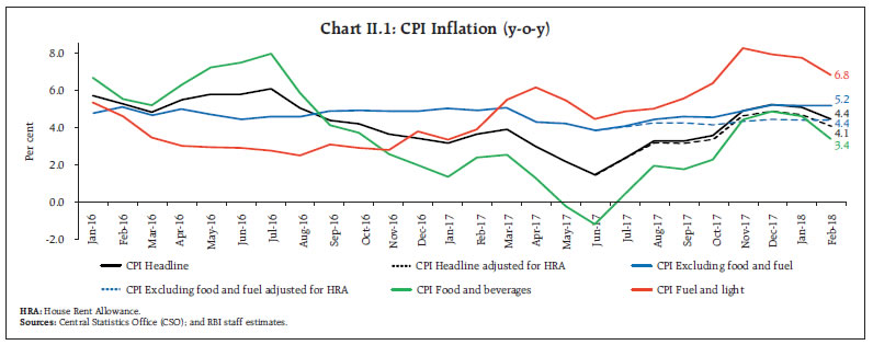 II.1 Consumer Prices The increase in HRA for central government employees, which became effective from July 2017 and continued to accumulate till December 2017, shaped the path of headline inflation during Q3, with unseasonal hardening of prices of vegetables, accentuating a spike to 4.9 per cent in November. While prices of vegetables did undergo a shallower than usual moderation in December, an unfavourable base effect came into play, pulling up inflation to a peak of 5.2 per cent in December. In Q4, headline inflation moderated with a fall in momentum due to a delayed but steep reversal in prices of vegetables (Chart II.3). The distribution of inflation across CPI groups in 2017-18 had striking similarities as well as divergences with last year’s experience. While median and modal inflation were similar, the continuing deflation in pulses gave the inflation distribution a considerable negative skew this year in contrast to the positive skew generated by high sugar and pulses inflation during 2016-17 (Chart II.4). Diffusion indices3 of price changes in CPI items suggest that on a seasonally adjusted basis, after an uptick in Q3:2017-18, the situation reversed in January-February, with the prices of a number of goods, particularly of food items, registering decline (Chart II.5).
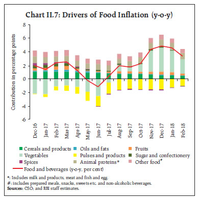
II.2 Drivers of Inflation A historical decomposition4 of inflation shows that the persistent effect of favourable supply shocks, especially on food prices, provided a cushion in the first half of 2017-18. However, the positive supply shocks waned in the second half of the year vis-á-vis the first half. The lagged impact of the still negative output gap and moderation in nominal rural wages also contributed to lower inflation during this period, while the firming up of crude oil prices imparted upward pressure (Chart II.6a). 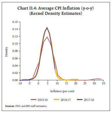 Decomposing inflation into its goods and services components reveals that the pick-up in inflation from June to December 2017 and its reversal from January 2018 largely emanated from prices of non-durables, particularly perishables; while those of services registered a sustained increase, primarily due to increase in housing inflation from 4.7 per cent in June to 8.2 per cent in December and further to 8.4 per cent in February, reflecting the statistical effect of the HRA (Chart II.6b). Housing alone contributed over 90 per cent of the observed increase in services inflation during this period. 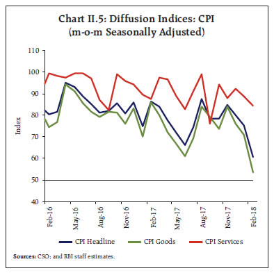 Turning to the drivers of food inflation in the second half of the year, the food and beverages sub-group contributed around 40 per cent to overall inflation, up from just 12 per cent during the first half. Adequate buffer stocks kept inflation in cereals generally under check. With cereals inflation under check, the pick-up in food inflation was largely on account of prices of vegetables – specifically tomato and onion – and intermittent uptick in prices of animal protein-rich food items. Continued decline in prices of pulses exerted a strong downward pull. Inflation in processed food products also moderated due to, inter alia, downward revision in GST rates (Charts II.7 and II.8). 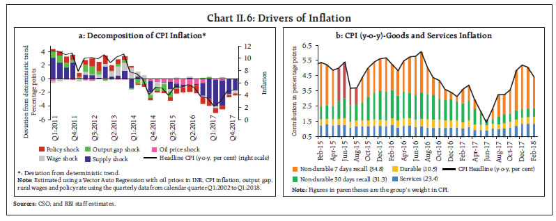
 Vegetables, which account for 13 per cent of the food group in CPI, were the principal drivers of food inflation. Price pressures in vegetables started building up from June 2017 following a fall in mandi arrivals, especially in onions and tomatoes (Chart II.9a). In the case of tomatoes, the upsurge in prices was so sharp that inflation in this category went up from (-)41 per cent in June 2017 to 119 per cent in November 2017 due to supply disruptions caused by adverse weather conditions – high temporal and spatial variability and delayed withdrawal of monsoon – and farmers’ agitation in parts of Maharashtra and Madhya Pradesh. While tomato prices recorded some contraction during August-September, the extended South-West monsoon in October in several important tomato-producing centres, especially in states like Karnataka, Andhra Pradesh, Telengana, Madhya Pradesh and Odisha, led to severe crop losses and tomato prices shot up again in November. 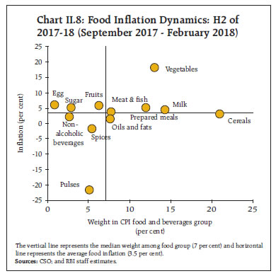 Another driver was the inflation in onions, which rose from (-)14 per cent in April 2017 to 159 per cent in December. Again, while unfavourable weather was a factor, large procurement of onions by a few state governments was the principal cause of the price spike. Post-November 2017, onion and tomato prices plunged with the arrival of fresh winter crops. Supply management measures by the government, especially in case of onions, helped in easing prices. The minimum export price (MEP), which is the key supply management measure used by the government to contain onion price surges, was re-implemented during the year in November and set at US$ 850 per tonne. The State-owned canalising agency viz., Metals and Minerals Trading Corporation of India (MMTC), imported 2,000 tonnes of onions, while other agencies such as National Agricultural Cooperative Marketing Federation of India (NAFED) procured around 10,000 tonnes of onions directly from the farmers, and the Small Farmers’ Agri-Business Consortium (SFAC) bought around 2,000 tonnes of onions locally and supplied to the consumers. The central government also advised states to take measures by way of licensing, imposition of stock limits and movement restrictions to balance supplies. In response, onion prices softened and the government brought down the MEP to US$ 700 per tonne in January 2018 before withdrawing it completely in February 2018. 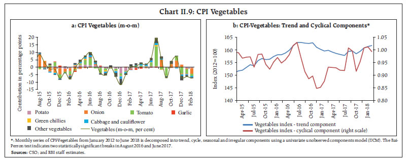 In case of potatoes, delayed sowing in West Bengal – a key growing state – due to extended monsoon showers in October, induced price pressures. However, carry-over stocks from the previous crop reined them in. Analysis based on CPI data suggests that there is no significant difference in the m-o-m changes of prices of vegetables in urban and rural areas – the spike in prices of vegetables uniformly impacted rural and urban India5. Most of the demonetisation-induced fall in prices of vegetables reversed as is evident from the trend and cyclical components of CPI-Vegetables (Chart II.9b). The other food components that recorded uptick in prices, albeit unevenly, were protein-rich items such as egg, meat and fish. Inflation in egg prices jumped from 0.8 per cent in October to 9.3 per cent in December, pushed up by tighter supply conditions on account of reduced egg production by poultry farms at the time of the usual increase in winter demand. Pulses, with a weight of 5 per cent in the food group, contributed significantly to food inflation dynamics during the year. The contribution of pulses to overall inflation shifted from 6.0 per cent during 2016-17 to (-)19.0 per cent in 2017-18. At a granular level, the contribution of arhar in overall pulses inflation declined consistently from July 2017, while the contribution of gram prices, turned increasingly negative month after month till December 2017. With the production for pulses during 2017-18, as per the second advanced estimates, being marginally higher at 23.95 million tonnes (23.13 million tonnes in 2016-17), pulses prices have now fallen significantly below trend levels (Charts II.10a & b). 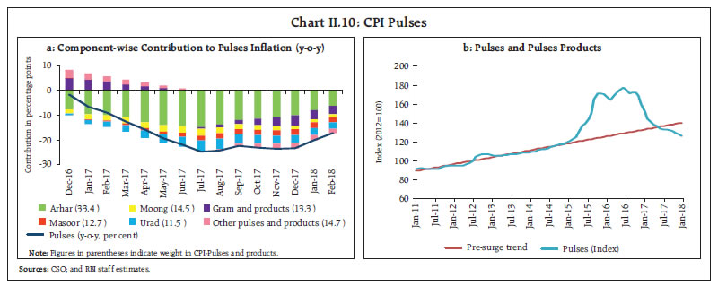
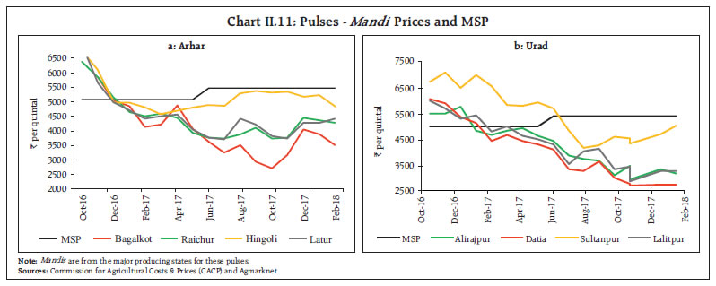 Arhar and urad prices remain below their minimum support prices (MSPs) at the mandi level in the major producing states viz., Maharashtra, Madhya Pradesh, Gujarat, Uttar Pradesh and Karnataka reflecting the large gap in procurement relative to supply (Chart II.11). Corrective measures were initiated by the government during the course of the year such as removal of export ban on all pulses and an imposition of 60 per cent import duty on gram and 30 per cent import duty on masoor in order to support prices and provide some relief to farmers. Sugar and spices are the other items which played an important role in the overall moderation of food inflation. Inflation in sugar and confectionery, which was in double digits all through 2016-17 (averaging about 20 per cent), declined significantly during the year, largely due to measures facilitating imports and on expectations of higher domestic production (the sugarcane production for 2017-18, as per the second advanced estimates, is 353.2 million tonnes as against 306.1 million tonnes in 2016-17). With sugar prices easing rapidly, however, the central government has again raised the import duty on sugar to 100 per cent and re-imposed stockholding limits on sugar sales for February and March 2018. Prices of spices have moved into deflation since June 2017 on account of a fall in prices of dry chillies, turmeric, dhania, and black pepper. Fuel and light inflation, which was at 5.0 per cent in August 2017, touched 8.2 per cent in November 2017, the highest since September 2013 (Chart II.12) largely on account of a sustained increase in domestic prices of LPG – tracking rising international product prices – as well as due to rural fuel consumption items such as dung cake. Since the migration of subsidy payments on LPG to banks under the direct benefit transfer scheme, LPG prices track international prices closely. Administered kerosene also registered sustained price increases as OMCs raised prices in a calibrated manner. Fuel and light inflation since December has eased driven by the downturn in LPG inflation, reflecting international price movements, as well as on account of moderation in firewood and chips and dung cake inflation. 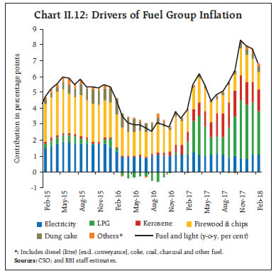
 Turning to the underlying inflation dynamics, CPI inflation excluding food and fuel edged up from the June 2017 trough of 3.8 per cent to 5.2 per cent in December and remained at that level during January- February 2018 – an increase of around 130 basis points between June and February (Chart II.13). The substantial increase largely reflected an increase in housing inflation (Chart II.14). Netting out the HRA impact, CPI inflation excluding food and fuel would have been 4.4 per cent – around 75 basis points lower than the observed print – during December 2017 to February 2018. Inflation in CPI excluding food and fuel, as also petrol and diesel, increased from June 2017 by 140 basis points to 5.3 per cent in February 2018. While the HRA impact explained much of this increase, petrol and diesel initially in Q3, had a dampening effect as much of the pass-through of surge in international crude oil price to domestic prices was delayed to the second half of January 2018. Furthermore, the excise duty cuts in early October 2017 by ₹2 per litre each for petrol and diesel also helped cushion the incremental impact of rising international crude prices (Chart II.15). Further, excluding the four volatile items – petrol, diesel, gold and silver – and housing, the inflation in February was 70 basis points lower at 4.4 per cent, and reflected the underlying inflation momentum in the second half of 2017-18. 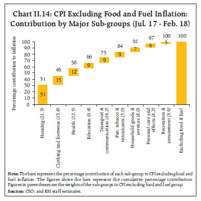 In H2:2017-18, both goods and services in CPI excluding food and fuel exhibited a rising inflation trajectory, notwithstanding some softening in case of goods in the recent months. For goods, inflation picked up across commodity groups: medicines under the health sub-group; clothing and footwear; pan, tobacco and intoxicants; and gold under the personal care and effects sub-group (Chart II.16a). Services inflation increased by 177 basis points over June (Chart II.16b), driven by housing sub-group due to the release of HRA from July 2017 under the recommendations of the 7th CPC. The contribution of transport services also edged up in recent months, as fuel prices were transmitted to increase in transportation fares. In contrast, communication services inflation has remained muted due to low cellular services inflation.
Other Measures of Inflation Measures of inflation other than CPI remained moderate in Q3 and Q4:2017-18. Inflation in wholesale price index (WPI) that does not include services, the CPI for rural labourers (RL) and the agricultural labourers (AL), which do not have housing components, moved in tandem with headline CPI up to October. The gap between inflation in terms of the CPI for industrial workers (CPI-IW) and the headline CPI, which was wide since July 2017 after HRA was implemented, closed in January 2018. CPI-IW adjusts its housing index only twice a year – in January and July. Thus, the HRA impact was reflected only in January 2018. GDP and GVA deflators also remained lower than CPI in Q3 (Chart II.17a). After the June 2017 trough, inflation measured by trimmed means in the CPI hardened for the rest of 2017. Thereafter, all trimmed means, including the weighted median, edged down, reflecting, inter alia, the broad-based softening of food prices (Chart II.17b). II.3 Costs Underlying cost conditions have mostly co-moved with measures of inflation, ticking up in H2:2017-18, notwithstanding some moderation in Q4. Y-o-y growth in farm input costs slipped temporarily into negative territory in January 2018 (Chart II.18). The rise in global crude oil prices and the hardening of metal prices fuelled the rise in input costs from August 2017 onwards and contributed to the turnaround in domestic non-farm input costs as they got passed on to inputs such as high speed diesel, aviation turbine fuel, naptha, bitumen, furnace oil and lube oils. Among other industrial raw materials, domestic coal inflation generally remained high during the year, tracking the surge in international coal prices and domestic supply shortages. However, inflation in other inputs depicted a mixed behaviour. In the case of oilseeds, inflation picked up during H2:2017-18, whereas in the case of fibres and paper and pulp, inflation moderated during the same period. Inflation in electricity, which carries a high weight in both industrial and farm inputs, rose during September-October 2017, but turned negative thereafter. Among other farm sector inputs, diesel prices increased sharply from August 2017, mirroring international prices, while prices of inputs such as tractors and fodder increased sharply in February 2018 after contracting in the preceding months. Fertiliser prices also recorded some upward pressure during December-February. 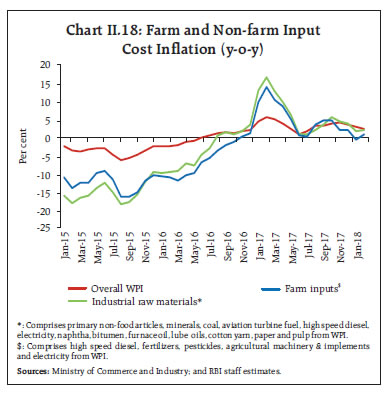
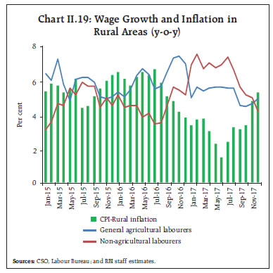 Growth in rural wages largely moderated since August 2017 (Chart II.19). In general, nominal rural wages and inflation tend to move together. However, large supply shocks have caused a divergence between the two in the recent period (Box II.1). Staff costs in the organised manufacturing sector rose between Q3:2016-17 and Q2:2017-18, but moderated during Q3:2017-18. The y-o-y growth in per employee cost for the manufacturing sector moderated to 11.6 per cent during Q3:2017-18. Staff costs in the services sector continued to decelerate from Q4:2015-16 till Q1:2017-18 and rose thereafter to 6.6 per cent in Q3:2017-18 (Chart II.20). Based on responses of manufacturing firms covered in the Reserve Bank’s industrial outlook survey, the cost of raw materials is assessed to increase significantly in Q4:2017-18 in relation to the previous quarter. Firms expect the cost of raw materials to rise further in Q1:2018-19, and pass them on to selling prices due to pressure on their margins. The manufacturing purchasing managers’ index (PMI) suggests that input costs accelerated in the second half of 2017-18, registering their highest level in February in the past 12 months before edging down in March. The co-movement of output prices with input prices suggests that pricing power is returning. In PMI services, there was a sharp acceleration in input prices in Q3, with the input services price index reaching its highest level of 55.0 since October 2013. The prices of services continued to increase in Q3 and Q4, though its momentum moderated with the downward revision in GST rates for many services. 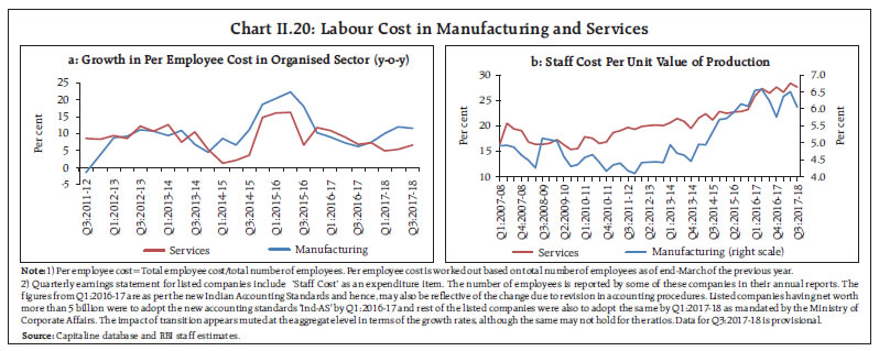
Box II.1: Relationship among Rural Wages, Inflation and Economic Activity: Recent Evidence Rural wages and inflation have moderated since early 2015, but with considerable divergence in their trajectories, particularly since July 2016 (Chart II.19). Historically, nominal wage growth and inflation tended to move together with inflation generally leading nominal wage growth, though with a slow speed of adjustment to disturbances (Kundu, 2018). An important issue that arises in this context is whether evolving economic activity has affected rural wages and inflation differently. Drawing on Knotek et al. (2014), two different Phillips curve specifications were estimated and compared to understand the differential impact of the output gap on rural wage growth and rural inflation. In the first specification, a wage Phillips curve with rural wage inflation as the dependent variable and economic activity measured by output gap (OG)6 as the independent variable was estimated: The second specification consisted of a price Phillips curve with CPI rural price inflation as the dependent variable and economic activity measured by OG as the independent variable: Both specifications were estimated for the period 2015 to 2017 for 15 major states. In the case of the rural wage Phillips curve, nine occupations7 were considered, while the CPI-Rural inflation Phillips curve was estimated with five major groups8. The regression results (Table II.1.1: Columns 1 and 2) show that while the rural wage Phillips curve holds for the recent period, i.e., economic activity is able to explain wage inflation, the price Phillips curve does not hold, i.e. economic activity is not able to explain CPI-Rural inflation9. However, in order to further analyse whether the price Phillips curve holds for a measure of underlying inflation rather than the overall inflation, which is often subject to large supply shocks from food and fuel prices, an alternate specification with CPI-Rural inflation excluding food and fuel as the dependent variable was also estimated: 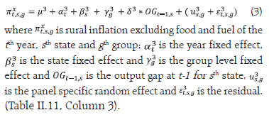
| Table II.1.1: Empirical Phillips curves | | Independent Variables | Dependent Variable | | Wage Inflation | CPI-Rural Inflation | CPI-Rural Excluding Food and Fuel Inflation | | (1) | (2) | (3) | | OG(-1) | 0.2709 | 0.0860 | 0.2712 | | | (0.052) | (0.436) | (0.007) | | State fixed effects | Yes | Yes | Yes | | Time fixed effects | Yes | Yes | Yes | | Group fixed effects | Yes | Yes | Yes | | No. of observations | 405 | 225 | 135 | Note: p-values in brackets.
Hausman test and Breusch and Pagan Lagrangian multiplier test suggest a random effect model. Regression equations are estimated using generalised least squares regression with AR(1) disturbances to overcome the presence of autocorrelation. Pesaran’s cross-sectional dependence test suggests that residuals are uncorrelated across panels. | In this case, OG is found to be statistically significant and of broadly the same magnitude as in the wage Phillips curve. Taken together, these results suggest that economic activity is a significant determinant of movements in both rural wages and CPI-Rural excluding food fuel inflation but not the overall CPI-Rural inflation (which includes both food and fuel). Rural food inflation since 2015 gyrated in a wide range of (-)0.8 per cent to 7.9 per cent, pointing to the outsized role of supply side shocks in driving recent food inflation trajectory that masks the underlying association between prices and economic activity. In other words, the recent divergence in rural wage growth and inflation could be explained by large supply side shocks affecting rural food inflation (Chart II.6a). References: Behera, H., Wahi, G., & Kapur, M. (2017), ';Phillips Curve Relationship in India: Evidence from State-Level Analysis';, RBI Working Paper Series No. 08/2017. Knotek II, E. S., & Zaman, S. (2014), ';On the Relationships between Wages, Prices, and Economic Activity';, Economic Commentary, Federal Reserve Bank of Cleveland, August. Kundu, S. (2018), ';Rural Wage Dynamics in India: What Role does Inflation Play?';, mimeo. | II.4 Conclusion Going forward, a key risk to the inflation outlook is the risk of fiscal slippages in a scenario of rising aggregate demand. As noted in the MPC resolution of February 2018, apart from the direct impact on inflation, the fiscal risks could also engender a broader weakening of macro-financial conditions. The revised guidelines for arriving at the MSPs for kharif crops proposed in the Union Budget 2018-19, along with proposed increase in customs duty on a number of items, is likely to push-up inflation over the year. In addition, how various state governments implement and disburse HRA increases would have a considerable bearing on CPI housing inflation and consequently on the headline inflation trajectory, albeit statistically, during 2018-19; therefore, the latter should be looked through for monetary policy purposes, other than for their second-round effects. Although the central government's HRA effects on CPI inflation would gradually wane from July 2018, this moderating impact could be more than offset if several state governments simultaneously implement HRA increases in H2:2018-19 (Chapter 1).
III. Demand and Output Aggregate demand growth accelerated in H2:2017-18, supported mainly by an investment upturn, while consumption remained resilient. Aggregate supply conditions were buoyed by the robust performance of the manufacturing sector and the improvement in activity in the agriculture and services sectors. Domestic economic activity shrugged off the loss of speed that had characterised the period Q1:2016-17 to Q1:2017-18 and a turning point appears to have taken hold in Q2-Q3, with lead indicators pointing to further acceleration in Q4. In terms of aggregate demand, the drivers around this inflexion are shifting, with consumption-led growth of the recent past handing over the baton to investment, which had restrained growth since Q3:2016-17. At the same time, the strong impetus from fiscal spending during Q3:2016-17 to Q1:2017-18 appears to be waning and the rapid pace of import growth is sapping net external demand. On the supply side, the pickup in industrial output from Q2:2017-18 and the strengthening of construction activity in the services sector from Q1 are noteworthy. Meanwhile, agriculture and allied activities have turned out to be resilient to temporary weather disruptions in both kharif and rabi sowing seasons and going by recent estimates of foodgrains production, the outlook appears better than before. III.1 Aggregate Demand Aggregate demand appears to have regained traction in H2:2017-18 after a prolonged slackening that stretched up to a 13-quarter low in Q1:2017-18. Measured by y-o-y changes in real GDP at market prices, it accelerated to 7.2 per cent in H2:2017-18 from 6.1 per cent in the preceding half of the year and 6.4 per cent a year ago. The turnaround in Q2:2017-18 and the steady gathering of speed thereafter are largely benefitting from a favourable base effect – a low base level a year ago – rather than a quickening of momentum, since q-o-q seasonally adjusted annualised growth rate (SAAR) slowed in Q3 and flattened in Q4 (Chart III.1). For the year 2017-18 as a whole, however, the second advance estimates (February 2018) of the Central Statistics Office (CSO) indicate that the pace of expansion of aggregate demand is still slower than in the preceding year. 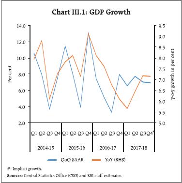 Turning to the underlying drivers, there are small but noteworthy shifts underway. In terms of weighted contributions, the support to aggregate demand from private consumption is waning, supplanted by the burgeoning strength of capital formation after a prolonged hiatus (Table III.1). This is significant since the historical experience has been that changes in capital accumulation are associated with level and/or slope shifts in India’s growth cycle. A surge in imports led to a higher negative contribution of net exports, which dragged down the overall demand. These developments are discussed in detail in the rest of this chapter. | Table III.1: Real GDP Growth | | (Per cent) | | Item | 2016-17 (FRE) | 2017-18 (SAE) | Weighted Contribution* | 2016-17 (FRE) | 2017-18 (SAE) | | 2016-17 | 2017-18 | Q1 | Q2 | Q3 | Q4 | Q1 | Q2 | Q3 | Q4# | | Private Final Consumption Expenditure | 7.3 | 6.1 | 4.1 | 3.4 | 8.3 | 7.5 | 9.3 | 4.2 | 6.6 | 6.6 | 5.6 | 5.6 | | Government Final Consumption Expenditure | 12.2 | 10.9 | 1.2 | 1.1 | 8.3 | 8.2 | 12.3 | 22.5 | 17.1 | 2.9 | 6.1 | 19.6 | | Gross Fixed Capital Formation | 10.1 | 7.6 | 3.1 | 2.4 | 15.9 | 10.5 | 8.7 | 6.0 | 1.6 | 6.9 | 12.0 | 9.9 | | Net Exports | – | – | 0.1 | -1.2 | – | – | – | – | – | – | – | – | | Exports | 5.0 | 4.4 | 1.0 | 0.9 | 3.6 | 2.4 | 6.7 | 7.0 | 5.9 | 6.5 | 2.5 | 3.0 | | Imports | 4.0 | 9.9 | 0.9 | 2.1 | 0.1 | -0.4 | 10.1 | 6.6 | 16.0 | 5.4 | 8.7 | 10.0 | | GDP at Market Prices | 7.1 | 6.6 | 7.1 | 6.6 | 8.1 | 7.6 | 6.8 | 6.1 | 5.7 | 6.5 | 7.2 | 7.1 | FRE: First Revised Estimates; SAE: Second Advance Estimates; #: Implicit growth.
*: Component-wise contributions to growth do not add up to GDP growth in this table because changes in stocks, valuables and discrepancies are not included.
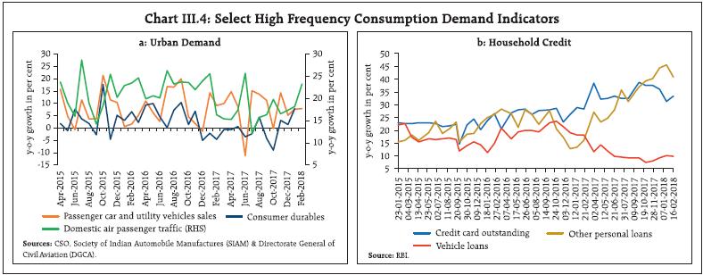
Source: Central Statistics Office (CSO). | III.1.1 Private Final Consumption Expenditure Private final consumption expenditure (PFCE) constituted 56.6 per cent of domestic demand in H2:2017-18, down from 57.5 per cent a year ago (Chart III.2). Short-term adverse effects of demonetisation and the implementation of the GST have taken their toll on output and employment in the unorganised sector, most vividly reflected in significant slowdown in exports of labour-intensive goods such as leather goods, textiles, jute manufactures, readymade garments. and sports goods (Chart III.3). Rise in global crude oil prices also appears to have contributed to the slowdown in private consumption.  High frequency indicators of urban consumption present a mixed picture. While consumer durables production remained subdued during the larger part of 2017-18, domestic air passenger traffic, and passenger cars and utility vehicles sales showed robust growth (Chart III.4a). Going forward, urban consumption is expected to strengthen with the likely implementation of the award on salaries and allowances at the level of states and other public sector entities. A sharp growth in personal loan portfolios of commercial banks and the recent pick-up in vehicle loans also augur well for urban consumption (Chart III.4b). The turnaround in construction activity – an employment-intensive sector in H2:2017-18 (as detailed later in the chapter) should support rural consumption. Indicators of rural demand, viz., growth in sales of two-wheelers and tractors remained strong, particularly from Q2. The production of consumer non-durables has also recovered markedly (Chart III.5a). 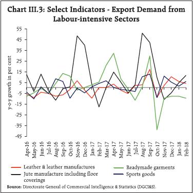
 III.1.2 Gross Fixed Capital Formation A stark feature of India’s recent growth experience has been the protracted downturn in investment, however, a turnaround set in during Q2:2017-18. Gross fixed capital formation (GFCF) strengthened further to touch a six-quarter high in Q3. The share of gross fixed capital formation in GDP, which was trapped in a downturn from a high of 34.3 per cent in 2011-12 to 30.3 per cent in 2015-16, broke free and increased to 31.4 per cent in 2017-18. As alluded to earlier, this pick-up in the investment rate could be signalling a turning point in the cyclical component of growth oscillations in India and if sustained by a determined policy push, it could produce a level shift in the trajectory of the Indian economy (Box III.1). Capital goods production – a key element of investment demand – turned around in August 2017 and clocked a 19-month high in terms of growth rates in January 2018 (Chart III.5b). During 2017-18 so far (up to December), the construction of highway projects is on the rise and is expected to have improved further in Q4. 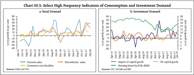
Box III.1: India’s Investment Cycle - Is It Turning? The slowdown in India’s growth over the past two years and the coincident slump in capital formation has generated significant concerns. The investment rate in real terms has slowed down after 2010-11 (Chart III.1.1a). With real GFCF growing at a slower rate, its contribution to real GDP growth declined from 44.4 per cent in 2016-17 to 36.1 per cent in 2017-18 (Chart III.1.1b). As changes in the rate of investment have been historically associated with turning points in the growth path, the trend and cyclical components of the investment rate and its duration of cycle were estimated by applying Hodrick-Prescott (HP) and Band-Pass (BP) filters. While there has been a moderation in the trend component of the investment rate since 2010-11, the cyclical component has shown an upward movement from the year 2016-17, suggesting that the recent improvement in investment activity is largely driven by cyclical factors (Chart III.1.2). 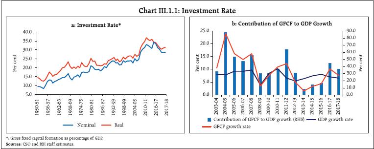
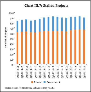
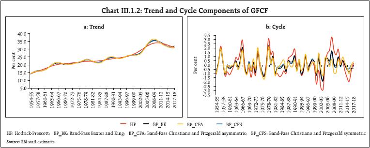 While there are two broad approaches for the measurement of business cycles, viz., the dating procedure and the production function approach, the first one is preferred and widely used in view of inherent problems associated with measurement of technology shocks through a production function framework. In this context, the business cycle and the growth cycle approaches developed by the National Bureau of Economic Research (NBER) are commonly used for the dating procedure. In the first method (Burns and Mitchell, 1946), the business cycle is measured by absolute changes in the general level of production in two steps: (i) identification of cyclical peaks and troughs in the observed economic variables; and (ii) determining whether these changes are common across all the observed series. In the second approach, a growth cycle is defined as the ups and downs in the deviations of the actual growth rate of the economy from the long-run trend growth rate (Zarnowitz, 1992). | Table III.1.1: Duration of Investment Cycle | | Cycle Reference Year | Duration (in Years) | | Peak | Trough | Contraction | Expansion | Cycle | | Peak to Trough | Previous Trough to this Peak | Trough from previous Trough | Peak from previous Peak | | - | 1950-51 | - | - | - | - | | 1951-52 | 1953-54 | 2 | 1 | 3 | - | | 1956-57 | 1958-59 | 2 | 3 | 5 | 5 | | 1959-60 | 1960-61 | 1 | 1 | 2 | 3 | | 1963-64 | 1964-65 | 1 | 3 | 4 | 4 | | 1966-67 | 1968-69 | 2 | 2 | 4 | 3 | | 1969-70 | 1970-71 | 1 | 1 | 2 | 3 | | 1971-72 | 1972-73 | 1 | 1 | 2 | 2 | | 1973-74 | 1976-77 | 1 | 1 | 2 | 2 | | 1978-79 | 1979-80 | 1 | 2 | 3 | 3 | | 1980-81 | 1981-82 | 1 | 1 | 2 | 2 | | 1982-83 | 1983-84 | 1 | 3 | 4 | 4 | | 1985-86 | 1986-87 | 1 | 2 | 3 | 3 | | 1987-88 | 1989-90 | 1 | 1 | 2 | 2 | | 1990-91 | 1991-92 | 1 | 1 | 2 | 2 | | 1992-93 | 1993-94 | 1 | 1 | 2 | 2 | | 1995-96 | 1996-97 | 1 | 2 | 3 | 3 | | 1999-00 | 2000-01 | 1 | 3 | 4 | 4 | | 2001-02 | 2003-04 | 2 | 2 | 4 | 3 | | 2004-05 | 2006-07 | 2 | 1 | 3 | 3 | | 2007-08 | 2009-10 | 2 | 1 | 3 | 3 | | 2010-11 | 2011-12 | 1 | 1 | 2 | 3 | | 2012-13 | 2015-16 | 3 | 1 | 4 | 2 | | 2017-18 | - | - | 2 | 2 | 5 | | Average | 1.4 | 1.6 | 3.0 | 3.0 | | Source: RBI staff estimates. | As the real GFCF rate has declined in levels on many occasions during the post-1950 period, identification of cyclical peaks and troughs in the observed levels of the economic variables based on the business cycle methodology, which is followed by NBER, is more suitable than the growth rate approach. For the purpose of measurement of the duration of investment cycle, the cyclical factor measured by Christiano and Fitzgerald asymmetric Band-Pass filter was used as it assigns variable weights and does not exclude end points. Following the business cycle approach of the NBER, it is observed that investment rate in India has gone through cycles of three-year (Table III.1.1). These results, when extrapolated, suggest that the upturn in the investment rate that commenced in Q3:2016-17 has approximately nine more quarters to fully play out. Policy efforts such as improving ease of doing business, speedy resolution of corporate distress, quickly addressing the remaining issues relating to the implementation of the Goods and Services Tax (GST) and speeding up of the stalled projects, among others, will help ride this phase of the investment cycle to its peak and produce accelerating impulses for the growth trajectory. Timely and measured interventions hold the key to realise the investment-led growth. References: Burns, A.F. and W.C. Mitchell (1946), Measuring Business Cycles, National Bureau of Economic Research, New York. Raj, Janak, Satyananda Sahoo and Shiv Shankar (2018), “India’s Investment Cycle – Is It Turning?”, Mimeo. Zarnowitz, V. (1992), Business Cycles Theory, History, Indicators and Forecasting, University of Chicago Press. | Corporate financial results are also mirroring these underlying shifts. The results of listed nongovernment non-financial (NGNF) companies suggest that manufacturing companies reduced current assets and increased fixed assets in H1:2017-18 vis-à-vis a year ago, possibly pointing to the long-awaited revival in the capex cycle. Nominal capex growth across 38 sub-sectors covering industrial and services sectors underwent a broad-based recovery in H1:2017-18 vis-à-vis H2:2016-17 (Charts III.6a and III.6b). A sharp pick-up in housing loans by scheduled commercial banks also augurs well for investment in dwellings. The implementation of stalled projects showed modest improvement (Chart III.7). 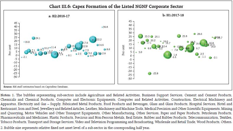
 Based on the CSO’s second advance estimates, gross fixed capital formation grew by 7.6 per cent in 2017-18 on top of 10.1 per cent in 2016-17. Seasonally adjusted capacity utilisation [CU(SA)], which remained below average since Q1:2013-14 due to overhang of excess capacity created during 2009-14, exhibited noticeable pick-up in Q3:2017-18 (Chart III.8). Going forward, large resource mobilisation from the primary capital market and accelerating non-food credit growth (Chapter IV) indicate that investment activity could strengthen further if fiscal pre-emptions do not crowd out private investment demand. III.1.3 Government Expenditure Government final consumption expenditure (GFCE) provided sustained support to aggregate demand in H2:2017-18, picking up in Q3:2017-18 on top of the front-loading of expenditure by the central government in Q1:2017-18. GFCE will likely continue to augment aggregate demand going forward into 2018-19, in view of the deviation of 0.3 per cent of GDP from the path of fiscal consolidation announced in the Union Budget (Table III.2). The gross fiscal deficit (GFD) target of 3.0 per cent of GDP has been deferred to 2020-21. In 2017-18 (April-February), there was a deterioration in the fiscal position of the central government on account of a sharp increase in expenditure combined with a decline in non-tax revenue relative to budget estimates. Revenue expenditure has evolved as budgeted, although payments under food and petroleum subsidies have been higher than a year ago. In the revised estimates for 2017-18, the outgo on account of major subsidies was estimated at 1.4 per cent of GDP, up from 1.3 per cent in 2016-17. Various categories of revenue expenditure take the form of committed payments with little room for cutbacks. Meanwhile, capital expenditure rose by 38.3 per cent up to February and constituted 108.6 per cent of the revised estimates (which were revised downwards from the budget estimates for the year). Accordingly, to meet the revised estimates, budgetary adjustments in the remaining part of the year might not involve any capex reduction, which has been stepped up over a wide area comprising civil aviation, defence, heavy industry, petroleum & natural gas, railways, shipping and road transport, including highways. | Table III.2: Key Fiscal Indicators - Central Government Finances | | Indicator | Per cent to GDP | | 2017-18 (BE) | 2017-18 (RE) | 2018-19 (BE) | | 1. Revenue Receipts | 9.0 | 9.0 | 9.2 | | a. Tax Revenue (Net) | 7.3 | 7.6 | 7.9 | | b. Non-Tax Revenue | 1.7 | 1.4 | 1.3 | | 2. Non Debt Capital Receipts | 0.5 | 0.7 | 0.5 | | 3. Revenue Expenditure | 10.9 | 11.6 | 11.4 | | 4. Capital Expenditure | 1.8 | 1.6 | 1.6 | | 5. Total Expenditure | 12.8 | 13.2 | 13.0 | | 6. Gross Fiscal Deficit | 3.2 | 3.5 | 3.3 | | 7. Revenue Deficit | 1.9 | 2.6 | 2.2 | | 8. Primary Deficit | 0.1 | 0.4 | 0.3 | Note: BE: Budget Estimates, RE: Revised Estimates.
Source: Union Budget, 2018-19. | Both gross and net tax collections were marginally higher than their budgeted levels, mainly on account of buoyant direct tax revenues under corporation tax (Chart III.9a). The budgeted buoyancies for all tax categories of direct taxes are higher in 2018-19 than the average of the preceding eight years (2010-11 to 2017-18), suggesting that revenue mobilisation would be a major challenge. Indirect tax collection during Apr-Feb. 2017-18 were higher by 12.9 per cent than their level a year ago (Chart III.9b). As per the Union Budget 2018-19, total revenue under GST for 2017-18 (RE) aggregated ₹ 4,446 billion. Collections under Centre GST (CGST) and integrated GST (IGST) were ₹ 2,214 billion and ₹ 1,619 billion, respectively. Non-tax revenues fell short of the budget target by 18.3 per cent due to lower receipts from dividends and profits as well as deferment of spectrum auctions. Total non-debt capital receipts were higher than the budget estimates (BE) by ₹ 330 billion on account of disinvestment proceeds, which exceeded the target of ₹ 725 billion. 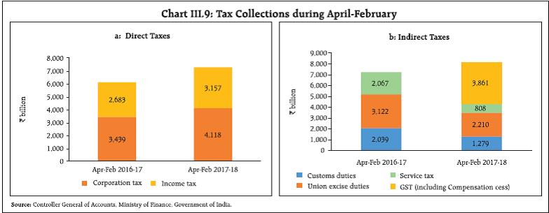 State finances have a significant bearing on the overall fiscal position of the general government. The latest available data for 21 States suggest a slippage in the combined GFD to gross state domestic product (GSDP) ratio to 3.0 per cent in 2017-18 (RE) as against 2.6 per cent budgeted (Table III.3). Revenue expenditures of states have shown significant divergences from budget estimates of 2017-18 so far, resulting from several factors such as implementation of the recommendations of states’ pay commissions, farm loan waiver in some states and rising interest burden (Chart III.10). This poses a challenge for overall fiscal consolidation. Though the budgeted fiscal deficit for 2018-19 for 21 states is placed lower at 2.5 per cent of GSDP, it is likely to come under pressure due to several factors such as upcoming state elections, likely farm debt waiver, and implementation of pay commission awards by some states. The borrowing programme of the Centre for 2017-18 was conducted at levels higher (1.4 per cent) than in the overall budgeted strategy, while States, at the aggregate level, borrowed less (13.4 per cent) than budgeted (Table III.4). A strategy of debt consolidation was undertaken through buybacks and switches to the extent of ₹ 416 billion and ₹ 581 billion, respectively. Gross market borrowings of the central government through dated securities for 2018-19 have been budgeted at ₹ 6,055 billion and net market borrowings at ₹ 4,621 billion. | Table III.3: Major Deficit Indicators – State Governments | | (Per cent to GSDP) | | Item | 2016-17 | 2017-18 BE | 2017-18 RE | 2018-19 BE | | Revenue Deficit | 0.4 | 0.0 | 0.4 | -0.1 | | Gross Fiscal Deficit | 3.4 | 2.6 | 3.0 | 2.5 | | Primary Deficit | 1.7 | 0.9 | 1.3 | 0.9 | Notes: 1. Negative (-) sign indicates surplus.
2. Data pertain to 21 out of 29 States.
Source: Budget Documents of State Governments. | The Centre’s gross fiscal deficit target of 3.2 of GDP for 2017-18 was exceeded by 0.3 percentage points of GDP. A slippage of the same magnitude has also been observed for states. Slippages in key deficit indicators have raised questions about the credibility of fiscal consolidation. In addition, higher fiscal deficits crowd out productive private sector investment. It is also worrying that revenue expenditure of the Centre for 2018-19 is budgeted to grow at a higher rate (10.2 per cent) than capital expenditure (9.9 per cent). In this context, even as the increase in outlays on agriculture and infrastructure proposed in the Union Budget for 2018-19 is welcome, concerted efforts need to be made to improve revenues. While disinvestment proceeds helped contain the fiscal deficit in 2017-18, they are contingent upon market conditions. It is important that tax revenues are maximised by expanding coverage and compliance, rationalising exemptions and building innate buoyancy so that the fiscal deficit budgeted for 2018-19 is adhered to without compromising the quality of the fiscal adjustment process. 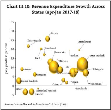
| Table III.4: Government Market Borrowings | | (₹ billion) | | Item | 2015-16 | 2016-17 | 2017-18 | | Centre | States | Total | Centre | States | Total | Centre | States | Total | | Net Borrowings | 4,406 | 2,594 | 7,000 | 4,082 | 3,426 | 7,508 | 4,484 | 3,403 | 7,887 | | Gross Borrowings | 5,850 | 2,946 | 8,796 | 5,820 | 3,820 | 9,640 | 5,880 | 4,191 | 10,071 | | Source: RBI. | III.1.4 External Demand Net exports continued to act as a drag on aggregate demand in H2:2017-18 with rapid import expansion outpacing exports (Charts III.11a and 11b). Although export growth slowed down to less than 3 per cent in H2:2017-18 from 6.2 per cent in H1:2017-18, there was a bounce-back in November and December with the easing of implementation hurdles associated with the GST. In Q4, however, there has been a sequential loss of pace, pointing to underlying weaknesses in the domestic supply response to rising external demand, especially in labour-intensive categories such as readymade garments, and gems and jewellery. Non-oil exports constitute a significant part of India’s exports, with engineering goods, and chemicals being consistent contributors through 2017-18 (up to January) (Chart III.12a). In line with trends in global trade, advanced economies (AEs) accounted for a larger share of the increase in India’s exports than emerging market economies (EMEs). Turning to imports, a large part of the strong growth was accounted for by non-oil non-gold imports during 2017-18 so far, attesting to the growing strength of domestic demand (Chart III.12b). Pearls and precious stones, electronic goods and coal1 were major contributors. Restocking by power plants and the growing requirements of the Indian steel sector led to an increase in coal imports in Q3:2017-18 to US$ 6.1 billion (56.8 million tonnes) from US$ 4.2 billion (44.8 million tonnes) in Q3:2016-17. Firming international crude oil prices on account of the Organization of the Petroleum Exporting Countries (OPEC) persisting with production cuts caused POL import bill to rise. Gold imports increased – both in value and volume terms – in December after declining in the preceding three months, but declined again in January 2018 due to the postponement of purchases in anticipation of reduction in customs duty on imports. Overall, merchandise import growth, which had largely declined sequentially up to October, started increasing strongly from November 2017, pushing the April-February trade deficit to a five-year high of US$ 143 billion. 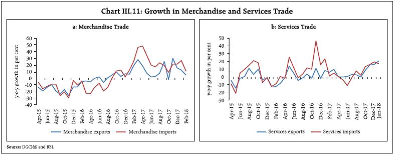
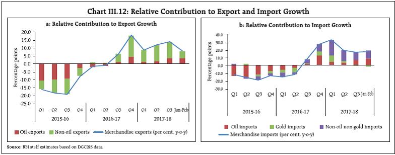 India’s net services exports picked up in Q3:2017- 18, mainly on account of improvement in exports of software and travel services. Despite the uncertainty relating to visa policies in the US and potential adverse effect of Brexit looming large, India’s software services recovered in key markets. The turnaround in global IT spending in 2017 also supported demand in this segment. The increase in net exports of travel services reflected the noteworthy rise in tourist arrivals in India. By contrast, increase in imports of services due to higher payments for travel, transport and business services partly offset the rise in export earnings. Remittances, which augment disposable income of households, also improved significantly in Q3, reflecting demand conditions in source countries. Even as global growth and trade accelerated in the recent period, the outlook is clouded by fears of rising trade protectionism. The direct impact of the recently announced tariffs by the US on India is likely to be modest; however, the increase in US tariffs may lead to a supply glut in non-US markets and push prices down, resulting in lower export realisation for India. The larger risk, however, is a possible escalation in trade protectionism around the world as the affected countries retaliate and protect domestic markets. This is already evident in the announcement of retaliatory tariffs on select US products by China after the US announced tariffs on Chinese goods. These actions may lead to global trade slowdown with hysteresis and diminished welfare, especially for countries looking to leverage on trade to meet their growth aspirations. The current account deficit (CAD) increased to 2.0 per cent of GDP (US$ 13.5 billion) in Q3:2017-18 from 1.4 per cent of GDP (US$ 8.0 billion) a year ago. The widening of CAD on a y-o-y basis was primarily on account of higher trade deficit (US$ 44.1 billion). All major components of capital flows, viz., foreign direct investments (FDI), foreign portfolio investments (FPI), non-resident Indian (NRI) deposits and external commercial borrowings (ECBs), recorded net inflows during Q3:2017-18. Gross as well as net FDI flows to India slowed in Q3 relative to preceding quarters. However, investors continued to prefer manufacturing and computer services, with Mauritius and Singapore remaining important sources. After bringing in robust inflows over the greater part of the year, foreign portfolio investors turned net sellers in the Indian equity and debt markets from the second week of February to the second week of March 2018, initially on anxieties relating to capital gains taxation proposals in the Union Budget and subsequently, in reaction to global sell-offs on fears of trade protectionism and faster pace of normalisation of US monetary policy. Going forward, these all factors may continue to impact portfolio flows to EMEs, although India’s resilient fundamentals and healthy level of foreign exchange reserves – at US$ 422.5 billion as on March 23, 2018 – should continue to provide buffers against global spillovers. III.2 Aggregate Supply Output growth in terms of gross value added (GVA) at basic prices accelerated to 6.8 per cent in H2:2017-18 from 5.9 per cent in H1 and 6.4 per cent a year ago, as the effects of demonetisation and teething troubles with the implementation of GST diminished gradually (Table III.5). GVA momentum, measured in terms of Q-o-Q SAAR, flattened in H2:2017-18 indicating that the acceleration of y-o-y growth in this period was due to a low base (Chart III.13). The turnaround in y-o-y GVA growth was underpinned by a sharp acceleration in industrial output, driven by manufacturing. Despite shortfalls in south-west and north-east monsoons, the growth in agricultural production picked up in comparison with H1:2017-18 and going by advance estimates of food grains, output scaled a record in 2017-18. Nevertheless, growth in agricultural activity slowed down relative to a year ago. Services sector activity, however, remained resilient. Significantly, GVA growth remained robust even after excluding public administration, defense and other services (PADO) (Chart III.14). 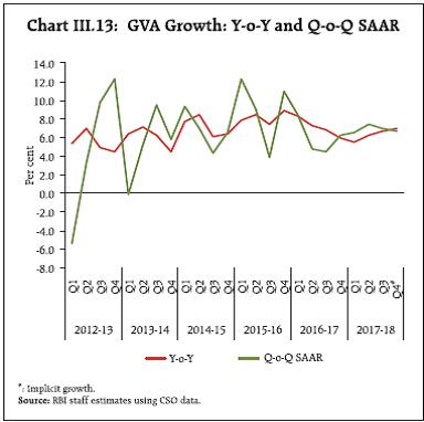
| Table III.5: Sector-wise Growth in GVA | | (Per cent) | | Sector | 2016-17 (FRE) | 2017-18 (SAE) | Weighted Contribution 2017-18 | 2016-17 (FRE) | 2017-18 (SAE) | | Q1 | Q2 | Q3 | Q4 | Q1 | Q2 | Q3 | Q4# | | Agriculture, forestry and fishing | 6.3 | 3.0 | 0.5 | 4.3 | 5.5 | 7.5 | 7.1 | 2.7 | 2.7 | 4.1 | 1.9 | | Industry | 8.7 | 5.0 | 1.2 | 10.2 | 7.8 | 8.8 | 8.1 | -0.4 | 7.0 | 6.8 | 6.8 | | Mining and quarrying | 13.0 | 3.0 | 0.1 | 10.5 | 9.1 | 12.1 | 18.8 | 1.8 | 7.1 | -0.1 | 3.9 | | Manufacturing | 7.9 | 5.1 | 0.9 | 9.9 | 7.7 | 8.1 | 6.1 | -1.8 | 6.9 | 8.1 | 7.2 | | Electricity, gas, water supply and other utilities | 9.2 | 7.3 | 0.2 | 12.4 | 7.1 | 9.5 | 8.1 | 7.1 | 7.7 | 6.1 | 8.4 | | Services | 6.7 | 7.8 | 4.8 | 8.5 | 7.4 | 6.0 | 4.9 | 8.6 | 6.6 | 7.6 | 8.3 | | Construction | 1.3 | 4.3 | 0.3 | 3.0 | 3.8 | 2.8 | -3.9 | 1.5 | 2.8 | 6.8 | 6.1 | | Trade, hotels, transport, communication | 7.2 | 8.3 | 1.6 | 8.9 | 7.2 | 7.5 | 5.5 | 8.4 | 9.3 | 9.0 | 6.7 | | Financial, real estate and professional services | 6.0 | 7.2 | 1.6 | 10.5 | 8.3 | 2.8 | 1.0 | 8.9 | 6.4 | 6.7 | 6.6 | | Public administration, defence and other services | 10.7 | 10.1 | 1.3 | 7.7 | 8.0 | 10.6 | 16.4 | 13.2 | 5.6 | 7.2 | 15.0 | | GVA at Basic Prices | 7.1 | 6.4 | 6.4 | 8.3 | 7.2 | 6.9 | 6.0 | 5.6 | 6.2 | 6.7 | 6.9 | FRE: First Revised Estimates; SAE: Second Advance Estimates; #: Implicit.
Source: Central Statistics Office (CSO). |
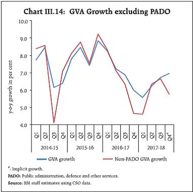 The October 2017 MPR had projected GVA growth of 6.4 per cent in Q2 and 7.4 per cent in H2 of 2017-18, with risks evenly balanced around the baseline path (Chart III.15). Actual outcomes in terms of the second advance estimates (SAE) of the CSO released on February 28, 2018 fell below these projections by 20 and 60 basis points, respectively. The deviation of SAE from the forecast for Q2 was primarily due to more than anticipated moderation in services sector activity, while in H2 it was accentuated by industrial activity also slowing down relative to expectations. Within industry, mining sector output contracted in Q3. Services sector growth slowed down due to an unanticipated contraction in sales growth in the real estate sector, following the implementation of the Real Estate (Regulation and Development) Act (RERA). Keeping these developments in mind, the GVA forecast for 2017-18 was revised downwards to 6.6 per cent in the MPC’s fifth bi-monthly statement of December 2017. 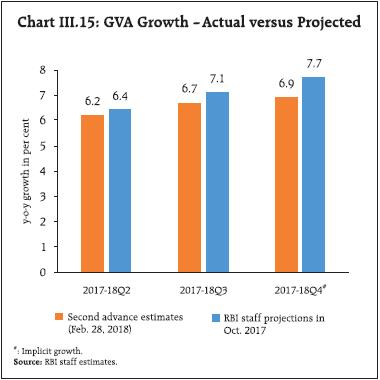 The advancement in the release of first advance estimates (FAE) of national accounts data by the CSO by more than a month in sync with the Union Budget has raised concerns about the firmness of GVA estimates, in view of the large gaps in data availability. Analysis of both production and expenditure-based estimates of national accounts suggests that during periods of rising growth, initial estimates were revised up in successive revisions, while during all periods of slackening of growth, they were revised down (see Box I.1 in Chapter I). Therefore, advance estimates of GDP/ GVA growth need to be supplemented with high frequency indicators to arrive at a realistic assessment of the state of the economy. III.2.1 Agriculture On a y-o-y basis, gross value added in agriculture and allied activities accelerated to 3.1 per cent in H2:2017-18 from 2.7 per cent in H1:2017-18, but decelerated significantly relative to H2:2016-17. The prolonged south west monsoon, better precipitation in the north-east monsoon (October-December 2017) relative to the preceding year, and comfortable water levels in major reservoirs ensured good soil moisture conditions for rabi sowing. However, delayed sowing, stubble burning, cold conditions and low prices hindered full acreage in the season, keeping it 0.8 per cent below last year’s coverage, mainly under wheat and oilseeds (mustard, rapeseeds). Consequent upon the release of the second advance estimates (SAE) of crop production for 2017-18, which indicated significant upward revision in the production of kharif crops and a better than expected rabi harvest, agricultural GVA growth for the year was revised upward to 3.0 per cent from 2.1 per cent in the FAE. Kharif foodgrains production for 2017-18 as per the SAE released in February 2018 was revised upwards by 2.8 per cent over the FAE released in September 2017. The SAE 2017-18 estimated foodgrains production at 277.5 million tonnes, 0.9 per cent higher than the previous record achieved in 2016-17 (275.1 million tonnes). The production of rice, pulses and coarse cereals touched new highs during the year, but wheat production declined (Table III.6). Going forward, average temperature in the central and eastern Pacific Ocean was in negative territory up to mid-February 2018 and turned positive since then, though the chances of an El Nino occurrence remain low. Horticulture production touched a record level of 305.4 million tonnes in 2017-18 as per the FAE, registering a growth of 1.6 per cent over final estimate of 2016-17. Subdued growth in fruits, vegetables, plantation and spices due to uneven spread of rainfall across major states held down a bigger supply response. Allied activities, which include forestry and fishing – contributing to around 41 per cent of total value addition in agriculture – grew by 5.1 per cent in FY 2017-18 (Chart III.16). III.2.2 Industrial Sector Gross value added in the industrial sector at basic prices accelerated to 6.8 per cent in H2:2017- 18 from 3.2 per cent in the preceding half, with the turnaround occurring in Q2, but was lower than the growth registered a year ago (Chart III.17). The slowdown in H2:2017-18 (so far) was due to a sharp deceleration in mining and quarrying (Chart III.18). In the mining sector, contraction was on account of slowdown in its key constituents such as coal and natural gas production, and decline in crude oil output (Chart III.19a). The growth of manufacturing, on the other hand, improved with the waning of the transient effects of GST to a five-quarter high of 8.1 per cent in Q3:2017-18. | Table III.6: Agricultural Production 2017-18 (Second Advance Estimates) | | (Million Tonnes) | | Crop | 2016-17 | 2017-18 | 2017-18 Variation (Per cent) | | SAE | Final Estimates | Target | SAE | Over SAE 2016-17 | Over Final 2016-17 | Over Target | | Foodgrains | 272.0 | 275.1 | 274.6 | 277.5 | 2.0 | 0.9 | 1.1 | | Rice | 108.9 | 109.7 | 108.5 | 111.0 | 2.0 | 1.2 | 2.3 | | Wheat | 96.6 | 98.5 | 97.5 | 97.1 | 0.5 | -1.4 | -0.4 | | Pulses | 22.1 | 23.1 | 23.0 | 24.0 | 8.2 | 3.5 | 3.5 | | Oilseeds | 33.6 | 31.3 | 35.5 | 29.9 | -11.0 | -4.4 | -15.8 | | Cotton # | 32.5 | 32.6 | 35.5 | 33.9 | 4.3 | 3.7 | -4.5 | | Jute & Mesta ## | 10.1 | 11.0 | 11.7 | 10.5 | 4.3 | -4.2 | -10.3 | | Sugarcane (Cane) | 310.0 | 306.1 | 355.0 | 353.2 | 13.9 | 15.4 | -0.5 | #: Million bales of 170 kgs. each: # #: Million bales of 180 kgs. each.
SAE : Second Advance Estimates.
Source: Ministry of Agriculture and Farmers Welfare. |
 GVA in the electricity sector moderated marginally in H2:2017-18 in comparison with H1. Growth in power generation during 2017-18 (April-February) was affected by lacklusture activity in thermal power plants (coal, diesel and gas-based plants), while hydro and nuclear power plants posted higher growth (Chart III.19b). The power sector is facing several handicaps such as coal shortages in thermal power plants; debt overhang of power distribution companies (DISCOMs); reluctance of some states to honour power purchase agreements, rendering projects unviable; and lower demand and pricing pressure being faced by thermal power plants in the wake of competitive pricing2 and rising popularity of renewable energy sources. 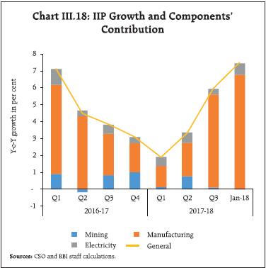 The strong performance of the manufacturing sector in Q3 was facilitated by robust sales growth that took the sector’s GVA growth to 10.9 per cent in nominal terms, while increasing raw materials costs were a drag. Of the 23 industry groups that form the manufacturing sector, production in 16 industries expanded during November-January 2017-18, indicating a wider base of output recovery. Among the major industry groups, the performance of coke and refined petroleum, chemical and chemical products, food products, machinery and equipment and other non-metallic mineral products turned around. Pharmaceuticals registered the highest growth (driven by digestive enzymes and antacids items), while electrical equipment remained in contraction mode throughout 2017-18 (April-January) (Chart III.20). 
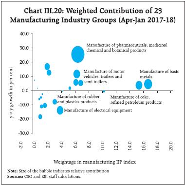 Exclusion-based measures, viz., truncated IIP and IIP excluding digestive enzymes and antacids (DEA), tracked overall IIP growth (Chart III.21a). In terms of weighted contributions, the acceleration was led by consumer non-durables, followed by capital goods (Chart III.21b). The latter could be indicative of a revival in investment demand that was reflected in disaggregated GDP data analysed in Section III.1.2. III.2.3 Services Activity in the services sector picked up and became broad-based in H2:2017-18, buoyed by a sharp acceleration in construction activity and support from PADO (Chart III.22a). The recovery in the construction sector was also reflected in the robust growth in steel consumption and cement production (Chart III.22b). The growth of financial, real estate and professional services, which had decelerated in Q2, improved marginally in Q3 but on the whole, growth decelerated in H2:2017-18 in comparison with H1. Though deposit growth remained muted, higher growth of credit pulled up overall financial services (Chart III.23a). Trade, hotels, transport and communication services continued to show robust performance in H2:2017-18. Lead indicators in the transport sub-segment – commercial vehicle sales, port cargo and air cargo traffic – showed an uptick in recent months (Chart III.23b). Similarly, indicators of the hotels sub-segment – foreign tourist arrivals and air passenger traffic, and communication – telephone and broadband subscribers, continued to grow strongly. The growth in PADO accelerated in H2:2017- 18, and especially in Q4, in the absence of cutbacks in expenditure by the central government. 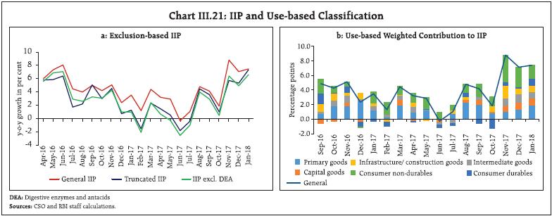
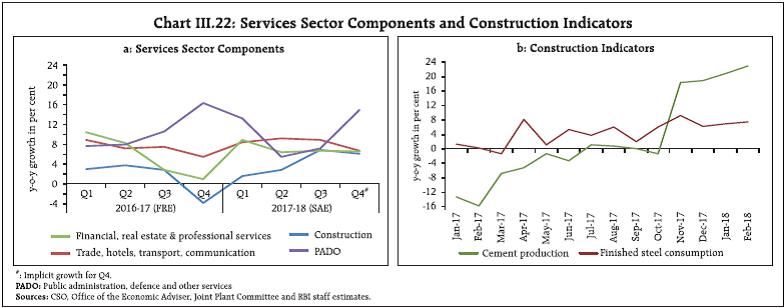 Indicators for real estate activity as reflected in sales and housing units launched, continued to decline across major cities as this sector is in the process of consolidation after the implementation of the RERA Act (Charts III.24a and III.24b). Developers are focusing more on completing and delivering existing projects rather than launching new projects. Weak demand and a large overhang of unsold inventory are other retarding factors. Listed real estate companies’ sales growth contracted by (-) 7.7 per cent in Q3 post-RERA. III.3 Output Gap An analysis of demand-supply conditions, which are important drivers of inflation, is an important input for monetary policy formulation. Apart from direct survey-based indicators such as measures of capacity utilisation, an estimate of demand-supply conditions is also made through an assessment of the output gap (i.e., deviation of actual output from its potential level and expressed as a proportion of potential output). Since potential output and the output gap are unobservable variables, and their estimates can be sensitive to the selected methodological approach, a variety of alternative approaches are used for assessing them. These include univariate filters such as the Hodrick-Prescott filter, the Baxter-King filter and the Christiano-Fitzgerald filter on the one hand, and multivariate Kalman filters on the other, that take into account inflation developments and/ or financial conditions to draw robust inferences on the state of the business cycle. 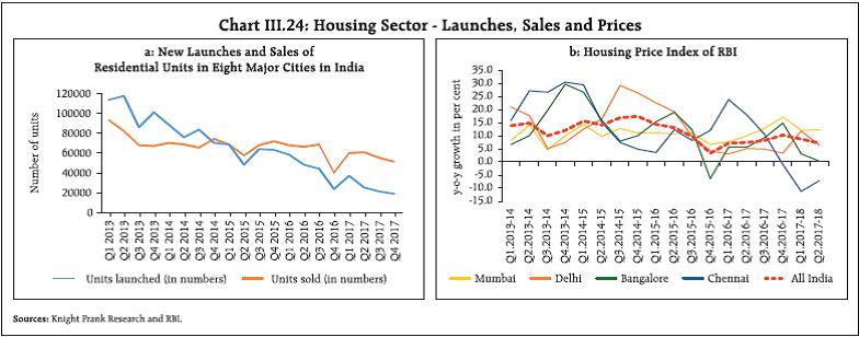 The composite estimate of the output gap, obtained by using principal component analysis on the various alternative estimates, indicates that the output gap is closing on account of strengthening of economic activity since Q2:2017-18 (Chart III.25a). This is consistent with a pick-up in domestic demand as reflected in rising capacity utilisation. The decomposition of the finance-adjusted output gap estimate shows that credit growth, supported by recapitalisation of public sector banks and deleveraging by the corporates under the Insolvency and Bankruptcy Code, and asset price growth, measured by Sensex, are contributing to the closing of the finance-adjusted output gap (Chart III.25b). III.4 Conclusion Economic activity, which was impacted on account of demonetisation and the implementation of GST, is recovering on the strength of an upturn in investment. A significant pick-up in credit off-take and larger resource mobilisation by the private sector in the recent period augur well for a fuller expansion of the investment cycle. Consumption demand remains robust and the focus of the Union Budget on the rural and infrastructure sectors should further support rural demand and investment. Global demand is also improving, which bodes well for India’s exports. The performance of manufacturing in the recent period has indeed been encouraging, especially as starting troubles relating to GST no longer bind. However, some concerns remain, which may have a bearing on growth prospects. First, the deterioration in public finances has the potential to crowd out private investment and potentially risks cutbacks on public capital expenditure. Second, recent firming up of international crude oil prices may reduce net external demand and also adversely impact profitability of domestic firms by raising input costs. Third, financial markets have become volatile in the recent period due mainly to global factors, and especially the uncertainty relating to trade protectionism and the pace of normalisation of monetary policy in advanced economies. Although global trade has been now growing faster than global growth, the fear of a trade war looms large and it has the potential to derail the ongoing global recovery. Therefore, the need to strengthen domestic macro-fundamentals assumes critical importance.
IV. Financial Markets and Liquidity Conditions Financial market conditions in the second half of 2017-18 were marked by the weighted average call money rate (WACR) moving closer to the policy repo rate as surplus liquidity moderated; stock markets scaling new highs before undergoing some corrections; firming up of bond yields; and, the foreign exchange market switching from buoyant to ebbing portfolio flows. As credit offtake picked up, monetary policy transmission gained further traction for new loans. Global financial markets generally remained buoyant through the second half of 2017, boosted by the improving macroeconomic outlook and the gradual normalisation of the US monetary policy. While equity markets surged on a renewed appetite for risk, currencies were lifted by the weakening of the US dollar since November. Yield curves in bond markets tended to flatten with still subdued inflation expectations, and corporate credit spreads narrowed. In 2018, however, market sentiment has been dampened by accelerating wage and employment growth in the US, triggering fears of a faster pace of interest rate increases. Longer term interest rates have been hardening tracking US yields, but also in response to country-specific developments. oscillating geo-political developments and more recent fears of a trade war in response to the US tariff announcements have heightened uncertainty considerably. Volatility has pervaded various market segments, with equity and bond market sell offs spilling across geographies. Currency markets have been hit by the turbulence of safe haven flights that are rotating capital flows among emerging economies and sporadically strengthening the US dollar. Financial markets have remained on edge in recent weeks. In domestic financial markets, various segments have exhibited diverse movements. While money markets remained laden with the overhang of liquidity that characterised the first half of the year, surplus liquidity has gradually ebbed and turned into deficit since February. As recourse to primary liquidity became pronounced from mid-December, overnight interest rates have begun ‘middling’ within the LAF corridor more frequently (Chart IV.1). Little farther out on the term curve, however, interest rates on Treasury bills (T-Bills) and discount rates on commercial papers (CPs) are hardening as markets sense that liquidity conditions are balancing out. In bond markets, long-term yields rose unrelentingly from August on apprehensions of excessive issuances, reactions to fiscal slippages following the announcement of the Union Budget for 2018-19, and rising inflation expectations peaking in early March. A spike in international crude price and rise in global interest rates contributed to the hardening of yields. Thereafter, yields declined sharply on favourable inflation print for February 2018 and in response to the lower than expected borrowings indicated by the Government in the issuance calendar for H1:2018-19. Corporate bonds also rose in sync, although credit spreads moderated with the improving outlook on growth. Until the Budget announcement, equity markets scaled new peaks, riding on aggressive buying by domestic mutual funds and foreign portfolio investors. Thereafter, corrections are occurring with bearish sentiment being more freely expressed in the equity market. The Union Budget proposal to levy long-term capital gains tax (LTCG) of 10 per cent on gains exceeding ₹1 lakh from sale of equity shares, sharp increase in US bond yields, the announcement of protectionist tariffs by the US and revelations of fraud in some domestic banks have impacted equity markets adversely since the beginning of February. The foreign exchange segment has moved in tandem; while the rupee had gained against the US dollar on the back of sustained portfolio inflows with the ebullience in equity markets, sentiment had reversed after the Budget announcement and portfolio outflows picked up from mid-February as global cues weighed on the rupee. In the credit market, activity is slowly gaining strength, despite the overhang of corporate loan delinquencies. The total flow of financial resources to the commercial sector in 2017-18 was much higher than that during the previous year, primarily due to an increase in non-food credit by banks. Credit demand surged in the second half of 2017-18 - though at divergent pace across bank-groups - with the growth pick-up spreading across sectors as underlying macroeconomic conditions improved. Both deposit and lending rates eased up to November as the cumulative reduction in the policy rate of 200 basis points since January 2015 was fully transmitted to new loans. IV.1 Financial Markets As set out above, domestic financial market segments have been mainly driven by idiosyncratic factors, barring phases of overwhelming global spillovers that impacted equity and forex markets intermittently. Excess liquidity, which had persisted till January following demonetisation, turned into deficit towards close of the year. Bond markets have experienced some drying up of liquidity as yields rose amidst concerns about inflation and the fiscal situation. The credit market, which was overcast with risk aversion and disintermediation, has exhibited a steady improvement in recent months with credit growth being in double digits since December. Sizeable investments by mutual funds into equity displaced the hitherto dominant position of foreign investors. IV.1.1 Money Market In the unsecured call money market, private banks and primary dealers are the major borrowers, and cooperative banks and public sector banks are the major lenders. In terms of intra-day activity, a distinct U-shaped pattern is discernible, with the thickest part of trading – more than 60 per cent of daily call money transactions _ occurring in the first hour (9-10 am) when primary dealers are most active as borrowers, and in the last hour (4-5 pm) when the call money market becomes the only source of market liquidity for banks and primary dealers. In both these time segments, public sector banks are the largest lenders. Co-operative banks accounted for 39 per cent of call money lending during the second half of 2017-18, down from 46 per cent in the first half. 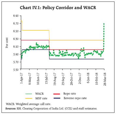 The demonetisation-induced slosh of liquidity hung heavily over the market in October and November. Amplified by the effects of the Reserve Bank’s forex operations, it continued to impart a downside bias to the weighted average call rate (WACR), as in the preceding two quarters (Chart IV.1). By mid-December, however, liquidity tightened with advance tax outflows. Restrained government spending impacted call money market conditions from February and firmed up interest rates. As net liquidity absorption under the LAF steadily shrank through the second half of 2017-18, the spread between the WACR and the policy repo rate narrowed from (-)13 basis points in September 2017 to (-)5 basis points in March 2018 (Chart IV.2). With the narrowing of the LAF corridor to 50 basis points in April 2017 from 100 bps earlier, volatility in the call money market has reduced, while the volume has remained broadly unchanged at less than 10 per cent of the total overnight market (Charts IV.3 and IV.4). 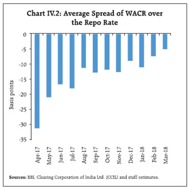 In the Collateralised Borrowing and Lending Obligation (CBLO) segment, which constitutes more than 60 per cent of the overnight market, banks are usually on the borrowing side, while mutual funds (MFs) are the major lenders. The share of MFs in CBLO lending, which had gone up to as much as 80 per cent in March 2017 in the wake of demonetisation, has gradually subsided during the year to more normal levels, averaging around 60-70 per cent up to March 2018. Intra-day trading is largely concentrated in the first hour in alignment with the call money segment and spikes around 1-2.30 pm due to stepped-up activity by associate members: market participants such as mutual funds and insurance companies who do not have current accounts with the Reserve Bank and are not allowed into the market beyond 2.30 pm (in order to provide for adequate time for settlement of fund obligations for these members who settle at designated settlement banks) (Chart IV.5). Trading volumes and rates fall sharply in the CBLO segment on reporting Fridays to escape the application of the cash reserve ratio (CRR)1. 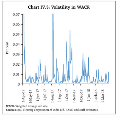
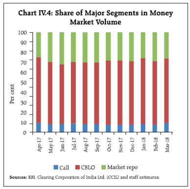 The collateralised market repo segment accounts for 30 per cent of the overall overnight market turnover. Typically, the turnover in the market repo segment comprises ‘basket repos’, in which foreign banks are the major lenders as they prefer market repo for lending because of its collateralised nature, and ‘specials’ that are used by market participants for acquiring specific securities to deliver against their outstanding short positions. In the second half of 2017-18, the shares of basket repo and special repo turnover in the market repo segment’s turnover were 55 per cent and 45 per cent, respectively, as against 57 per cent and 43 per cent in the first half. Interest rates in the collateralised segments, i.e., CBLO and market repo, evolved with a soft bias relative to the WACR and, in fact, traded 10 basis points and 2 basis points, respectively, below the WACR on average through the second half of 2017-18. 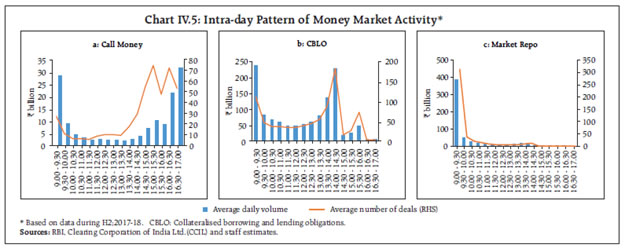 Barring term premia, interest rates on certificates of deposits (CDs), commercial paper (CPs) and 91-day Treasury bills (T-Bills) generally evolve in alignment with the WACR (Chart IV.6). From mid- December, however, they have diverged on higher interest rates for lending beyond March-end on the consideration of year-end demand for funds for balance sheet management purposes – a usual seasonal phenomenon – though this divergence was initially triggered by the announcement of additional market borrowing by the government. In recent years, CPs have been increasingly resorted to as credit substitutes for working capital requirements as CP rates continue to rule significantly lower than bank lending rates. Consequently, issuances of CPs picked up to ₹11,448 billion in the second half of 2017-18 as against ₹9,125 billion a year ago. As surplus liquidity shrank, fresh issuances of CDs also went up to ₹2,181 billion from just ₹1,017 billion in the second half of 2016-17.  IV.1.2 Government Securities Market Since the beginning of August 2017, yields in the secondary government securities (G-sec) market hardened almost monotonically, driven mostly by domestic factors up to early March 2018 (Chart IV.7). G-sec yields hardened by 20 bps in October mainly due to informal communication by the government in late September that gross fiscal deficit (GFD) could be higher, increase in inflation forecast by the monetary policy committee (MPC) on October 4 and concerns over increase in the supply of papers in the form of bank recapitalisation bonds announced on October 24, 2017. G-Sec yields hardened by 20 bps during November 2017 partly due to fiscal concerns.2 Moody’s rating upgrade on November 17, 2017 and the cancellation of open market sales scheduled for November 23, provided transient relief to the market. In December, the upside tilt in the balance of risks set out in the resolution of the MPC on December 6, concerns about rising inflation following December 12 release of inflation print and the communication on December 27, 2017 that fiscal slippage will be funded by additional market borrowings by the central government led to a rise in yields by 27 bps. Among global factors, rising international crude prices through the quarter and the increase of 25 basis points in the federal funds target on December 13, 2017 meeting of the FOMC pushed up the G-sec yields. On the whole, G-sec yields rose by 67 bps during Q3:2017-18. Over the same period, US yields rose by 8 bps. 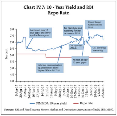 In Q4, notwithstanding the announcement of reduction of additional borrowings by the central government by ₹300 billion (from the amount of ₹500 billion extra borrowing announced in December) on January 17, 2018, the upward pressure on yields resumed from mid-January as still elevated crude prices and spillovers from episodes of global bond sell-off accentuated fears of oversupply of domestic paper. These fears materialised with the fiscal slippage announced in the Union Budget on February 1. Yields traded with a tightening bias till early March, scaling a two-year peak of 7.81 per cent on March 5, 2018. However, yields softened sharply by around 45 bps thereafter due to the lower inflation print for February released on March 12 and the decision by the Government not to front-load its borrowings in H1:2018-19 which resulted in a sharp fall in G-sec yields of 29 bps in a single day on March 27, 2018. As a result, the 10-year yield softened by 7 bps in Q4:2017-18 as against a rise of 36 bps in US yields. Reflecting these developments, the yield curve underwent level shifts through the second half of 2017-18, including in respect of the new benchmark paper issued on January 5, 2018 (Chart IV.8). An empirical analysis suggests that the sensitivity of bond yields in India to global factors represented by the US bond yield has declined in the recent period (although it has risen gradually since Q3), while its responsiveness to domestic factors has increased. Time-varying parameter estimates indicate that the effect of inflation on bond yields in India has increased significantly, especially since August 2017 (Chart IV.9)3. 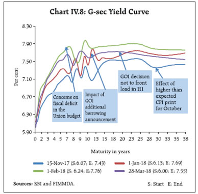
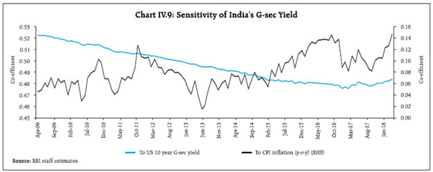 Persisting positive yield differentials between global (US treasuries) and Indian G-secs and the stability of the Indian rupee in the foreign exchange market relative to other currencies provided congenial conditions for foreign portfolio investors (FPIs) who were net buyers in the debt market during the most part of H2 (Chart IV.10), notwithstanding intermittent reversals following the Budget announcement. FPIs made investment of ₹606 billion in G-secs in 2017-18, resulting in utilisation of 92.9 per cent of the extant limit on G-sec investment. In addition, FIIs also made investment in state development loans (SDLs) of ₹40 billion. In the primary segment, two discerning features characterised opposite ends of the spectrum. At the short end of the G-sec market, T-Bill issuances declined during H2 with the steady improvement in the central government’s cash balances. Yields on T-Bills, however tracked the benchmark and hardened till February before cooling down during March owing to surplus liquidity emerging from the redemption of T-Bills issued under Market Stabilisation Scheme (MSS) in April-May 2017 (Chart IV.11). 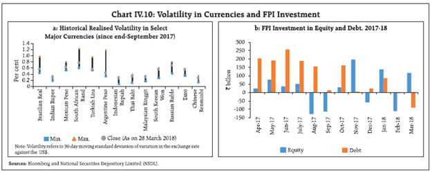
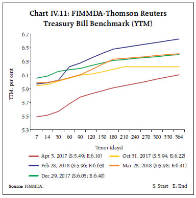 At the longer end, the issuances of SDLs moderated in Q3, partly in reaction to the tightening financial conditions in the bond market. However, issuances peaked in Q4 reflecting the increased expenditure by the States towards end of the financial year. The weighted average spreads over the 10-year G-sec yield moderated to 56 bps in H2 as compared with 63 bps in H1 (Chart IV.12). There were no issuances under the UDAY scheme during 2017-18 and the total secondary market trading volume (face value) of UDAY bonds was ₹898 billion. Following the recommendations of the 14th Finance Commission, all states (barring Delhi, Madhya Pradesh, Kerala and Arunachal Pradesh) have been excluded from the National Small Savings Fund (NSSF) financing facility beginning 2016-17. Consequently, market borrowings of states increased, also triggered by large redemptions of past borrowings. This drove up the supply of SDLs, which in turn impacted yields in the bond market, already reeling under the pressures of oversupply of paper. The relationship between the spread on SDLs and fiscal situation of individual States remained weak during 2017-18. The inter-state spread during the year at 6 bps was marginally lower than that of 7 bps in 2016-17. IV.1.3 Corporate Bond Market Corporate bond yields hardened during H2:2017- 18 tracking the rising G-sec yields (Chart IV.13a). In contrast, credit spread, i.e., the spreads of corporate bond yields over G-sec yields of corresponding maturity narrowed from September 2017 onwards, barring intermittent spikes during December and January. The spreads of 5-year AA rated corporate bonds yields declined by 16 basis points, reflecting improvement in financing conditions on the back of higher corporate earnings in a brightening macroeconomic outlook, and with the prospects of speedy resolution of insolvency under the bankruptcy code. Empirical analysis suggests that credit spreads increase with amplification of credit risks as captured through credit default swap (CDS) spreads, and increase in global liquidity risks measured by the Libor-OIS spread. However, spreads reduce with an increase in earnings prospects as reflected in 12-month forward price-to-earning-ratios4. Average daily turnover in the corporate bond market increased to ₹75.6 billion during H2:2017-18 (up to March 27, 2018) from ₹70.6 billion a year ago; however, the tightening of credit conditions reflected in hardening of corporate bond yields during H2: 2017-18 prompted corporates to shift to banks for meeting their funding requirements. Consequently, resource mobilisation through issuances of corporate bonds in the primary market declined by 15.9 per cent to ₹2,105 billion during October 2017-February 2018 from ₹2,502 billion during the same period of 2016-17 (Chart IV.13b). The share of financial entities in the resource mobilisation was 76 per cent during October 2017–February 2018. Almost the entire resource mobilisation from the corporate bond market (99.9 per cent) was by way of private placements. FPI in corporate bonds increased from ₹1.98 trillion at end- September 2017 to ₹2.24 trillion as on March 28, 2018, constituting 91.9 per cent of the approved limit for investment in corporate bonds. IV.1.4 Stock Market Equity markets extended their gains in H1:2017-18 into H2, with the Sensex closing at a historic high of 36,283 on January 29, 2018. A number of factors contributed to the market’s overall buoyancy: strengthening macroeconomic conditions; revival of corporate sales and improving prospects for future earnings; the announcement of PSU banks’ recapitalisation; a jump in India’s ranking in the World Bank’s ease of doing business index; the ratings upgrade by Moody’s; sustained net investment by domestic institutional investors; and positive cues from global equity markets. 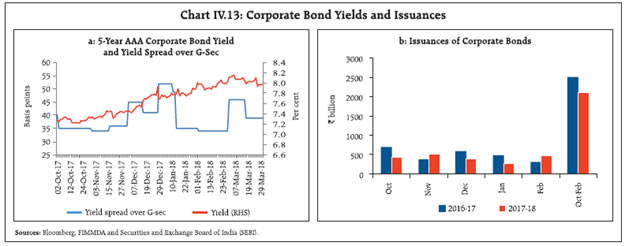 Market conditions and sentiment reversed dramatically in February and selling pressures intensified, with a variety of factors in play: global sell-offs in bonds and equities following stronger than expected job and inflation data for the US that prompted market participants to anticipate a faster pace of normalisation of US monetary policy; expectations of tighter liquidity conditions going forward; bearish sentiment post the Union Budget proposal to levy long-term capital gains tax (LTCG) of 10 per cent on gains exceeding ₹1 lakh from sale of equity shares; the breach in the fiscal deficit target for 2017-18 and for the medium term; and disclosure of fraudulent transactions by Punjab National Bank (Chart IV.14). Consequently, even though the BSE Sensex gained by 5.4 per cent during H2:2017-18, it declined by 5.0 per cent during the month of February and suffered losses of 3.6 per cent in March as well on worries of trade wars triggered by the announcement of tariffs on steel and aluminium imports by the US administration and plan to impose tariff on Chinese goods.  The sharp increase in equity indices in the second half of January 2018 and the dramatic correction in the first half of February 2018 were both associated with heightened volatility (Chart IV.15a). The increase in volatility during the first week of February 2018 resulted from spillover of enhanced volatility in global markets, as rising bond yields triggered sell-off in stocks, which was exacerbated by collapse of several complex volatility-linked funds and algorithmic trading strategies tied to market volatility.5 The India volatility index (VIX)6, which captures short-term expected volatility of Nifty 50, increased sharply during this period. While equity indices and the VIX are generally inversely correlated, they moved in tandem during the second half of January 2018 with the correlation co-efficient being 0.88. Global markets also witnessed a similar aberration as the S&P 500 and VIX moved together with a correlation co-efficient of 0.70. The put-call ratio, an indicator of market expectations, broadly remained stable and stayed below one in India. These configurations suggest that equity markets in India had perhaps risen excessively and that a correction – rather than a bearish phase – was imminent. As if in corroboration, the sharp correction in equity indices led to the restoration of the inverse relationship between the VIX and NIFTY 50 in February 2018, with the correlation co-efficient being -0.31. Realised volatility estimated through GARCH conditional volatility remained consistently lower than the expected volatility (measured by the VIX) during this period (Chart IV.15b). 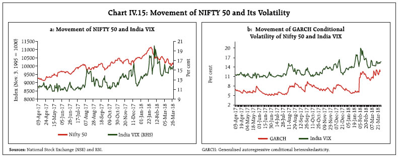 While domestic institutional investors, particularly MFs, engaged in sustained net buying in the equity market, foreign portfolio flows experienced some volatility in February. Net investment by mutual funds in equities during October 2017 to March 27, 2018 at ₹631 billion was higher than that of ₹302 billion by foreign portfolio investors (Chart IV.16). During October 2017-February 2018, resources raised under equity-oriented investment schemes were higher at ₹841 billion than ₹399 billion during the corresponding period of the previous year. This reflected greater participation not only from retail and high net worth individuals (HNIs), but also from corporates. Equity assets under management (AUM) of mutual funds increased by 16.7 per cent from ₹6.6 trillion at end-September 2017 to ₹7.7 trillion at end- February 2018. In the primary segment of the equity market, resource mobilisation through public issues of equity (initial public offers and right issues) increased sharply to ₹610 billion during October 2017-February 2018 from ₹100 billion in the corresponding period of the previous year. Of the total 71 initial public offer (IPO) issues, 53 issues were listed on the small and medium enterprises (SMEs) platforms of BSE Ltd. and National Stock Exchange (NSE). Of the total resource mobilisation by way of public equity issues during 2017-18, 50.4 per cent was raised by insurance companies. IV.1.5 Foreign Exchange Market The Indian rupee experienced intermittent bouts of volatility during H2:2017-18. Concerns over political turmoil in the Middle East and the concomitant knock-on impact on international crude oil prices drove the rupee lower against the dollar during the first two weeks of November 2017. A weakening US dollar and robust foreign portfolio investor (FPI) purchases in the Indian debt market supported the rupee through December and early January (Chart IV.17a). In the latter part of January and in February, the re-emergence of concerns around the repercussions of elevated energy prices on India’s trade deficit, anxiety around recalibration of the speed of monetary policy tightening by the Federal Reserve upon arrival of strong wages and employment data, and the introduction of LTCG tax in India subjected the rupee to downward pressure. This was accentuated by the strengthening of the US dollar and sales by FPIs in the equity and debt markets. Net purchases by FPIs from mid-March 2018 supported the rupee. Overall, the rupee appreciated marginally from its end-September 2017 levels in contrast to currencies of peers that are running current account deficits (Chart IV.17b). The Indian rupee depreciated in nominal terms against a basket of 36 currencies of trading partners between September 2017 and March 2018 (Table IV.1). In real terms also, the rupee depreciated, although the extent of depreciation was lower than in nominal terms, reflecting inflation differentials. | Table IV.1: Nominal (NEER) and Real Effective Exchange Rates (REER): Trade-based (Base: 2004-05=100) | | Exchange Rate | Index: end-March 2018 (P) | Appreciation (+)/Depreciation(-) (Per cent) March 2018 over September 2017 | | 36-currency NEER | 74.9 | -2.0 | | 36-currency REER | 117.4 | -1.5 | | 6-currency NEER | 65.0 | -3.4 | | 6-currency REER | 124.4 | -3.2 | P: Provisional.
Note: REER figures are based on the Consumer Price Index (Combined).
Source: RBI. |
Currencies of peer economies such as South Africa, Malaysia, China and South Korea, among others, appreciated in real terms, while those of the Philippines and Turkey depreciated (Chart IV.18). IV.1.6 Credit Market After remaining depressed for nearly two years, non-food credit built upon the uptick that started around June 2017 and expanded in double digits from December 2017. The resurgence in credit growth was observed across bank groups, though the pace of growth continues to vary among bank groups. The year-on-year growth rate of bank credit for scheduled banks was 11.1 per cent as on March 16, 2018. Credit extended by private sector banks and public sector banks grew by 21.5 per cent and 6.7 per cent, respectively. Credit extended by foreign banks has returned to positive territory after a year-long contraction (Chart IV.19). 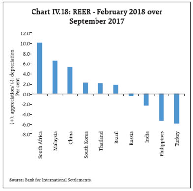
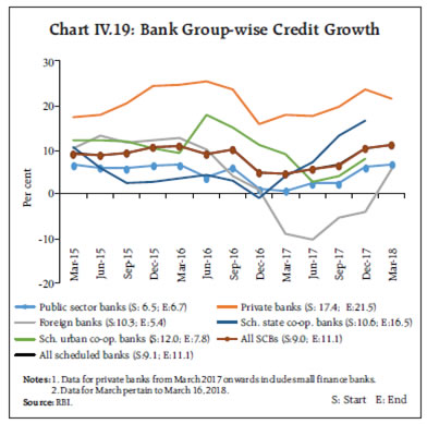 Credit growth is also becoming increasingly broad-based (Chart IV.20), with offtake by industry turning positive after a protracted period of contraction. The industry sub-groups that registered the sharpest improvement in credit flow on a y-o-y basis as of February 2018 include mining and quarrying, food processing, textiles, chemicals, rubber, leather, glassware and engineering industries. With a pick-up in the traditional form of financing through loans, resource flow to the commercial sector of the economy by way of non-SLR investments (investment in commercial paper (CP) and bonds/ shares/debentures issued by non-financial corporates) by banks declined in 2017-18 (Chart IV.21). Concomitant with the reduction in surplus liquidity in the system, pick-up in credit growth as also rising risk of fluctuations in government bond yields, investment in government securities by banks over and above the prescribed statutory liquidity ratio (SLR) declined through H2. The banking system as a whole maintained excess SLR by 8.2 per cent of their net demand and time liabilities (NDTL) as on March 2, 2018 (Chart IV.22). The total flow of financial resources to the commercial sector in 2017-18 (up to March 16, 2018) was higher than in the comparable period a year ago (Chart IV.23). While funding from the banking sector increased by 33 per cent, that from the non-bank sector (including domestic and foreign sources) increased marginally by 2 per cent. It needs to be noted that data on most non-bank sources of funding are available with a lag. Overall funding provided by banks and non-banks to the commercial sector improved by 14 per cent. 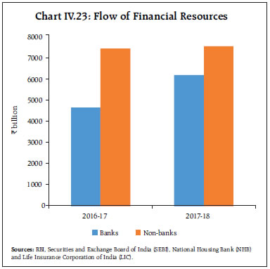
| Table IV.2: Funding from Non-Bank Sources to the Commercial Sector | | (Amount in ₹ billion) | | Item | April to mid-March | | 2016-17 | 2017-18 | | Amount | Per cent to Total | Amount | Per cent to Total | | A. Flow from Non-banks (A1+A2) | 7,336 | 100.0 | 7,491 | 100.0 | | A1. Domestic Sources | 5,114 | 69.7 | 4,869 | 65.0 | | 1 Public issues by non-financial entities $ | 120 | 1.6 | 380 | 5.1 | | 2 Gross private placement by non-financial entities $ | 1,804 | 24.6 | 1,273 | 17.0 | | 3 Net issuance of CPs subscribed to by non-banks | 1,465 | 20.0 | 462 | 6.2 | | 4 Net credit by housing finance companies # | 761 | 10.4 | 1,117 | 14.9 | | 5 Total accommodation by 4 RBI regulated AIFIs $ | 192 | 2.6 | 708 | 9.4 | | 6 NBFCs-ND-SI (net of bank credit) * | 541 | 7.4 | 588 | 7.8 | | 7 LIC’s net investment in corporate debt, infrastructure and social sector $ | 230 | 3.1 | 341 | 4.6 | | A2. Foreign Sources | 2,222 | 30.3 | 2,622 | 35.0 | | 1 External Commercial Borrowings / FCCB @ | -467 | -6.4 | -108 | -1.4 | | 2 Short-term credit from abroad * | 167 | 2.3 | 604 | 8.1 | | 3 Foreign Direct Investment to India @ | 2,523 | 34.4 | 2,126 | 28.4 | #: Up to Nov. *: Up to Dec. @: Up to Jan. $: Up to Feb.
Sources: RBI, SEBI, NHB, LIC, BSE, NSE and merchant banks. | Apart from banks, the main sources of domestic funding for the commercial sector during 2017-18 were the corporate debt market (private placement of debt), housing finance companies, the four RBI-regulated all India financial institutions (AIFIs) and non-banking financial companies (NBFCs) (Table IV.2). Further, funding through public issues increased sharply; as a result, their share in total funding increased by more than three-fold. Foreign direct investment and short-term credit from abroad were the main sources of foreign non-bank funding to the commercial sector, with the latter showing a sharp over three-fold increase. Even as the stressed assets ratio of banks has stabilised, the overall level of gross non-performing assets in the system has continued to rise, especially in the case of industry due to the continuing improvement in asset quality recognition at banks (Chart IV.24). This overhang has been one of the factors that has held down the surge in growth rate of loan books of public sector banks. 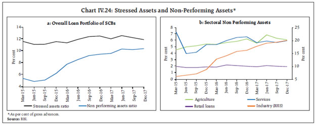
|
|
| Table IV.3: Transmission to Deposit and Lending Rates | | (Variation in percentage points) | | Period | Repo Rate | Term Deposit Rates | Lending Rates | | Median Term Deposit Rate | WADTDR | Median Base Rate | 1 Yr Median MCLR | WALR - Outstanding Rupee Loans | WALR - Fresh Rupee Loans | | January 2015 to March 2018 | -2.00 | -1.65 | -2.04 | -0.80 | * | -1.59 | -1.90 | | April 2016 to March 2018 | -0.75 | -0.95 | -1.13 | -0.20 | -1.05 | -0.95 | -0.92 | | Memo: | | | | | | | | | Pre-Demonetisation | | | | | | | | | January 2015 to october 2016 | -1.75 | -0.99 | -1.26 | -0.61 | * | -0.75 | -0.97 | | April 2016 to october 2016 | -0.50 | -0.29 | -0.35 | -0.01 | -0.17 | -0.11 | 0.01 | | Post-Demonetisation | | | | | | | | | November 2016 to March 2018 | -0.25 | -0.66 | -0.78 | -0.19 | -0.88 | -0.84 | -0.93 | WADTDR: Weighted average domestic term deposit rate. WALR: Weighted average lending rate. MCLR: Marginal cost of funds based lending rate system.
Latest data for WADTDR and WALR pertain to February 2018.
*: MCLR system was put in place on April 1, 2016.
Source: RBI. | IV.2 Monetary Policy Transmission The surge in low cost current account and savings account (CASA) deposits into the banking system post demonetisation, coupled with the aggressive reduction in term deposit rates, aided the pass through of policy rate cuts to lending rates of commercial banks (Table IV.3). The speed of transmission gathered momentum from November 2016, with lending rates falling faster than term deposit rates. This also reflected the still subdued demand for credit and the availability of alternative non-bank sources of financing. The extent of reduction in lending rates on outstanding loans continued to be relatively small though, due to sticky interest rates on base-rate- linked loans and the 1-year reset period of MCLR-linked loans. Since January 2015 – when the accommodative cycle of monetary policy commenced – the median base rate has declined by 80 basis points (bps) as against the cumulative decline of 200 bps in the policy repo rate. Significantly, the pace of decline in the base rate slackened drastically after the introduction of the MCLR in April 2016. As the proportion of outstanding loans linked to the base rate (which were contracted during July 2010 – March 2016) declined only gradually through 2016-17 and in 2017-18, the transmission of policy rate cuts to outstanding loans amounted to 55 bps during 2017-18 (up to February), albeit higher than 40 bps during 2016-17. As a result, the monthly median spread between the WALR and one-year MCLRs of individual banks declined after scaling a peak in January 2017 (Chart IV.25). 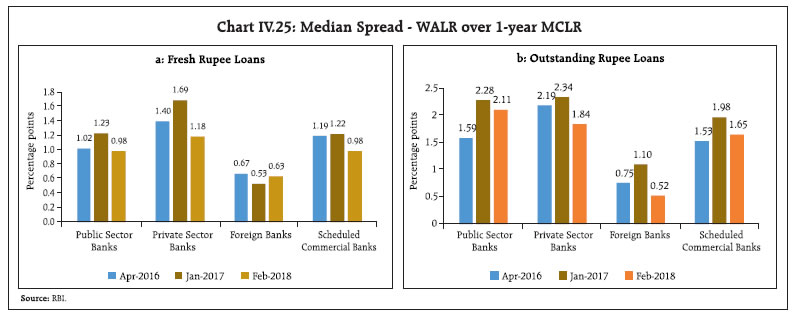 The asset quality of banks plays a significant role in keeping the spread (over the MCLR/base rate) low. With deterioration in asset quality, banks tend to charge higher spreads by loading higher credit risk premia while pricing loans, thereby impeding monetary transmission. A study in this regard confirms this observed behavioural relationship (Box IV.1). Box IV.1: Asset Quality and Monetary Transmission Efficient monetary transmission is contingent upon the health of the banking system, particularly in a bank-dependent financial system such as in India (Table IV.1.1). Asset quality could impact monetary transmission by amplifying/retarding the effect of changes in short-term policy/money market interest rates on lending interest rates as well as by changing banks’ lending standards and their use of non-price measures while sanctioning loans. The impact of asset quality on monetary transmission can be captured by net interest margin (NIM), which is the difference between interest income and interest expenditure (in relation to total assets). In the presence of gross non-performing assets (NPAs), transmission may be impeded if banks charge higher NIM to account for higher credit risk while maintaining their profitability (return on assets) at the targeted level. This would mean that during the easing phase of monetary policy cycle, banks will not lower their lending rates in line with the reduction in their cost of funding (John, et al, 2018). | Table IV.1.1: Share of Banks in the Flow of Resources to the Commercial Sector | | (Per cent) | | Year | Domestic and Foreign Sources | Domestic sources | | 2007-08 | 44.1 | 63.5 | | 2008-09 | 47.3 | 58.5 | | 2009-10 | 45.0 | 56.7 | | 2010-11 | 56.9 | 70.2 | | 2011-12 | 55.7 | 68.7 | | 2012-13 | 48.1 | 61.7 | | 2013-14 | 54.0 | 63.9 | | 2014-15 | 45.5 | 55.2 | | 2015-16 | 51.3 | 61.3 | | 2016-17 | 34.9 | 43.2 | | 2016-17 (Up to Feb 2017) | 38.3 | 48.5 | | 2017-18 (Up to Feb 2018) | 42.9 | 53.5 | | Source: RBI, SEBI, NHB and LIC. | In the Indian context, a question has arisen as to whether the deterioration in asset quality of banks in the recent period has had any adverse impact on monetary transmission. To test this hypothesis, Arellano-Bover/ Blundell-Bond dynamic panel GMM model was used with time and bank fixed effects employing quarterly data on 72 banks – 26 public sector banks, 19 private sector banks and 27 foreign banks _ for the period 2010- 11 Q1 to 2017-18 Q1. Estimates reveal that credit risk, proxied separately by the gross NPA to total assets ratio and the stressed assets to total assets ratio resulted in increase in NIM of scheduled commercial banks (Table IV.1.2)7. This suggests that deterioration in asset quality indeed impacted monetary transmission in India. The regression was initially conducted for the full sample period (Q1:2010-11 to Q1:2017-18). However, the impact of asset quality on NIM appeared to differ between (a) Q1:2010-11 to Q1:2015-16 (sub-period I); and (b) Q2:2015-16 to Q1:2017-18 (sub-period II). | Table IV.1.2: Determinants of Net Interest Margin of SCBs Dependent Variable: NIM | | | Full Sample | Sub-Period I | Sub- Period II | | (1) | (2) | (3) | (4) | | Gross NPA | 0.0057* | 0.0211*** | –0.0202*** | | operating Expense | 0.5066*** | 0.4313*** | 0.5444*** | | CRAR | 0.0006* | 0.0013*** | –0.0085*** | | observations | 2088 | 1512 | 576 | ***: Significant at 1% level; *: significant at 10% level.
Notes: Model Specification: Arellano-Bover/Blundell-Bond dynamic paneldata regression-system GMM with time and bank fixed effects.
NIM = (Interest income minus interest expense) to total assets (in per cent).
The regressions control for seasonality, lags, bank size, capital adequacy, return on assets, operating expense and non-interest income.
Hansen test for over identification restrictions and Arellano-Bond test for residual auto correlations are found to be satisfactory. Gross NPAs and operating expense are expressed as per cent to total assets.
Source: Staff estimates, Supervisory Returns, RBI. |
Table IV.1.3: Determinants of NIM – Bank Group-wise (Full Sample)
Dependent variable: NIM | | | Scheduled Commercial Banks | Public Sector Banks | Private Sector Banks | Foreign Banks | | (1) | (2) | (3) | (4) | (5) | | Gross NPA | 0.0057* | –0.0128*** | 0.0097 | 0.0123 | | operating Expense | 0.5066*** | 0.5614*** | 0.6585*** | 0.4870*** | | CRAR | 0.0006* | 0.0007 | 0.0024 | 0.0007 | | observations | 2088 | 754 | 551 | 783 | | Note: Refer to notes in Table IV.1.2. | During the first sub-period, the impact of the gross NPA ratio on NIM was positive and statistically significant, indicating that when NPA ratios were at a lower level, albeit rising, and credit growth was relatively strong, banks were able to charge additional risk premia to compensate for credit risk. During the second subperiod, the coefficient of the gross NPA ratio turned negative and statistically significant, suggesting that banks were not able to pass on the entire burden of NPAs to their new borrowers in the form of higher credit risk premium. Also, during this sub-period, the asset quality review (AQR) driven reclassification of restructured loans as NPAs prevented banks from recognising interest income on outstanding NPAs. Therefore, these findings suggest that in a competitive market, there are limits up to which banks could compensate themselves for a high degree of credit risk by charging additional risk premium for making provisions and achieving targeted returns on assets. Divergent behaviour was also observed for the three bank groups _ public, private and foreign – for the full sample period. While gross NPAs were found to have a negative impact on NIMs of public sector banks, they had a positive but statistically insignificant impact on NIMs of private sector and foreign banks. Since NPAs of public sector banks were at a much higher level than those of two other bank groups, the bank group-wise analysis corroborates the findings of the sub-period analysis that at higher levels of NPAs banks could not compensate themselves by charging higher credit risk premium (Table IV.1.3). The sub-period-wise and bank group-wise analyses suggest the presence of non-linearities imposed by the gross NPA ratio in determining the impact of credit risks on NIM. To ascertain a non-linear relationship between the gross NPA ratio and NIM, it was attempted to estimate the regression for the full sample period by introducing slope dummies for the gross NPA ratio.8 It was found that the slope is positive and statistically significant when the level of gross NPA ratio is low, and negative and statistically significant when the gross NPA ratio is higher. In summary, the findings support the bank group-wise and sub-period wise analyses i.e., at low levels of NPA ratio, banks are able to load the costs on to lending rates and protect NIMs, but not so at a higher level of NPAs. Reference: John, Joice, A.K. Mitra, Janak Raj and D. P. Rath (2018), “Asset Quality and Monetary Transmission in India”, Reserve Bank of India Occasional Papers, forthcoming. | In continuation of the past pattern of pricing of sectoral credit, commercial banks charged the lowest spread (over and above the base rate/MCLR) on housing sector mortgages and the highest spread for personal loans (other than housing, vehicle and education), which have an unsecured component (Chart IV.26). The low spread on housing loans could be attributed to the stiff competition from the non-bank sector and low default rates in this sector (Chart IV.27). High quality corporate bond yields continued to remain below the MCLR, making the former a relatively attractive instrument for raising resources by top rated corporates (Chart IV.28). 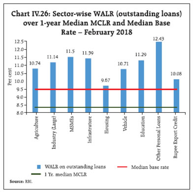 After the policy rate cut of 25 bps on August 2, 2017, the MCLR declined across tenors and across bank groups till February. During March, however, the MCLR was increased for all tenor by commercial banks. The benchmark tenor for MCLR is one year in the case of all public sector banks and most private sector banks, whereas it is dispersed across maturity buckets, including overnight and one-month tenors in the case of foreign banks10. Tenor-wise, the transmission was largest for the overnight tenor, followed by the onemonth tenor for commercial banks (Chart IV.29a). Among bank groups, the transmission to weighted average lending rate (WALR) and weighted average domestic term deposit rate (WADTDR) was largest in the case of public sector banks, followed by foreign banks and private sector banks (Chart IV.29b). 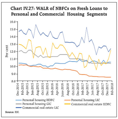
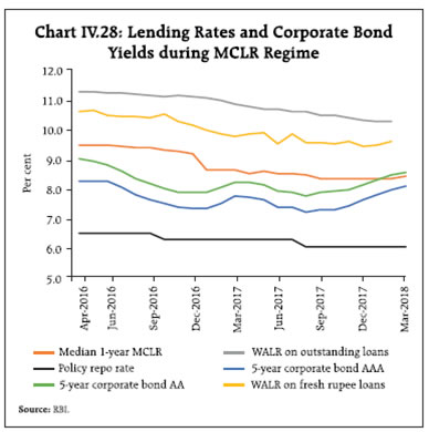 Since December 2017 and January 2018, respectively, deposit and lending rates have begun to inch up in line with interest rates in other financial market segments. With the transition of system-level liquidity from surplus towards neutrality, banks have started raising their interest rates in a sequence beginning with bulk term deposit rates, retail term deposit rates and on to MCLRs. The reduction in the share of current account and savings account (CASA) deposits of banks from 40.9 per cent in September 2017 to 39.8 per cent in mid-March 2018 could also be exerting upward pressure on the cost of funding (Chart IV.30). The one-year median MCLR of private sector banks and foreign banks increased by 10 bps and 5 bps, respectively, during January-February 2018. Further, the one-year median MCLR of both public sector banks and foreign banks increased by 5 bps and 3 bps, respectively, during March. With the WADTDR rising by 10 bps during December-February, WALR on fresh rupee loans and WALR on outstanding rupee loans of commercial banks too increased by 14 bps and 3 bps, respectively, from their lows reached in December and January, respectively. 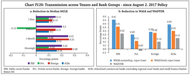 One of the factors that impedes transmission is the higher interest rates on small saving instruments. On March 28, 2018, the Government decided to keep the interest rates on small savings unchanged for Q1:2018-19 from those notified for Q4:2017-18. As a result, interest rates on some small savings schemes are now, for the first time, lower than those prescribed under the formula for fixing small saving interest rates and are better aligned with term deposit interest rates of banks (Table IV.4). IV.3 Liquidity Conditions and the Operating Procedure of Monetary Policy The Reserve Bank’s approach to managing large and persisting liquidity surpluses in the postdemonetisation period was set out in the Monetary Policy Reports of April and October 2017. Pro-active liquidity management measures undertaken in H2: 2017-18 drew upon this framework. During Q3, the Reserve Bank deployed variable rate reverse repo auctions of tenors ranging from overnight to 28 days and conducted open market sales on three occasions to absorb ₹300 billion on a durable basis (₹200 billion in October and ₹100 billion in November) in addition to the regular mopping up of liquidity through LAF fixed rate reverse repo. Accordingly, net average daily absorption of liquidity under the LAF declined from ₹1,400 billion in October 2017 to ₹718 billion in November, also aided by the ongoing increase in currency in circulation and pick-up in credit growth. Liquidity conditions temporarily turned into deficit mode in the second half of December with the slowdown in government spending prolonging the shortfall created by the usual advance tax outflows. Liquidity amounting to ₹1,315 billion was injected through variable rate repos of varying tenors in addition to regular 14-day term repos. | Table IV.4: Interest Rates on Small Savings Instruments for Q1:2018-19 | | Instrument/Scheme | Maturity (years) | Spread (Percentage point) $ | Average G-sec yield (Per cent) of corresponding maturity (December 2017 to February 2018) | Formula based rate of Interest (Per cent) (applicable for April to June 2018) | GoI Announced Rate of interest (Per cent) (applicable for Apr to June 2018) | Difference (Percentage point) | | (1) | (2) | (3) | (4) | (5) = (3) + (4) | (6) | (7) = (6) - (5) | | Savings Deposit | - | | | | 4.00 | - | | Public Provident Fund | 15 | 0.25 | 7.67 | 7.92 | 7.60 | -0.32 | | Term Deposits | | | | | | | | 1-Year | 1 | 0 | 6.36 | 6.36 | 6.60 | 0.24 | | 2-Year | 2 | 0 | 6.58 | 6.58 | 6.70 | 0.12 | | 3-Year | 3 | 0 | 6.81 | 6.81 | 6.90 | 0.09 | | 5-Year | 5 | 0.25 | 7.25 | 7.50 | 7.40 | -0.10 | | Post office Recurring Deposit Account | 5 | 0 | 6.81 | 6.81 | 6.90 | 0.09 | | Post office Monthly Income Scheme | 5 | 0.25 | 7.21 | 7.46 | 7.30 | -0.16 | | Kisan Vikas Patra | 118 Months | 0 | 7.67 | 7.67 | 7.30 | -0.37 | | NSC VIII Issue | 5 | 0.25 | 7.45 | 7.70 | 7.60 | -0.10 | | Senior Citizens Saving Scheme | 5 | 1.00 | 7.25 | 8.25 | 8.30 | 0.05 | | Sukanya Samriddhi Account Scheme | 21 | 0.75 | 7.67 | 8.42 | 8.10 | -0.32 | $: Spreads for fixing small saving rates as per Government of India Press Release of February 16, 2016.
Note: Compounding frequency varies across instruments.
Sources: Government of India and staff estimates. | In Q4, surplus liquidity declined with intermittent deficits on account of the drying up of government spending and large tax collections. The Reserve Bank resorted to fine-tuning variable rate auctions on both sides, in addition to the regular operations. Average daily net liquidity absorbed under Liquidity Adjustment Facility (LAF) (including Marginal Standing Facility (MSF)) declined from ₹2,667 billion in Q2 to ₹812 billion in Q3 and further to ₹30 billion in Q4. Consequently, the weighted average call rate (WACR) inched closer to the repo rate (Chart IV.31). During Q4, the liquidity situation moved from absorption mode during January – with average daily net liquidity absorbed under LAF (including MSF) amounting to ₹353 billion – to injection mode during February and March amounting to ₹60 billion and ₹213 billion, respectively. The WacR touched a high of 6.67 per cent on March 28, 2018 on the back of usual year-end increased demand for liquidity. Currency in circulation reached the pre-demonetisation level during the week ended March 9, 2018 (Chart IV.32). Anticipating tightness in liquidity conditions in March and with a view to providing greater flexibility to the banking system to tide over the usual year-end liquidity mismatches, four additional variable rate repo operations (₹250 billion each) of longer tenors (24 to 31 days) were conducted and standalone primary dealers (SPDs) were allowed to participate within the usual notified amount of the regular term repo auction conducted on March 28, 2018. Furthermore, liquidity was augmented in March through redemption of T-Bills, which were issued under the Market Stabilisation Scheme (MSS) in April and May 2017. 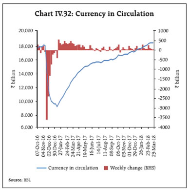 The amended RBI Act, 1934 enjoins the Reserve Bank to place the operating procedure of monetary policy and changes therein from time to time in the public domain. The Union Budget 2018-19 has proposed an amendment to Section 17 of the RBI Act, 1934 which would allow the Reserve Bank of India to accept “money as deposits, repayable with interest, from banks or any other person under the Standing Deposit Facility Scheme, as approved by the Central Board, from time to time, for the purposes of liquidity management.” The Standing Deposit Facility (SDF) as and when introduced will provide an additional mechanism for draining liquidity, particularly during periods of exceptional liquidity glut (Box IV.2). IV.4 Conclusion Equity and bond markets remain vulnerable to episodic bouts of volatility in a period of considerable uncertainty surrounding the evolution of global financial markets as well as around domestic developments which can impact market sentiment and liquidity conditions significantly, as the year gone by has shown. In the forex market, global developments – particularly in the systemically important economies – will continue to influence exchange rate developments, especially through the magnitude and direction of capital flows. Credit growth is accelerating and is also becoming broad-based, which bodes well for sustaining the pick-up in domestic economic activity that appears to have taken root since Q3. Going forward, liquidity conditions would be managed in a manner consistent with the Reserve Bank’s policy stance of moving towards ex ante neutrality in order to facilitate closer alignment of the operating target of monetary policy – the WACR – with the policy repo rate. Issues in monetary transmission will continue to engage the Reserve Bank and market participants, and efforts will be carried forward towards bringing in greater transparency in the setting of interest rates by banks. Box IV.2: Standing Deposit Facility The SDF will be an additional instrument of liquidity management for the Reserve Bank. It provides symmetry to the operating framework of monetary policy by introducing a standing absorption facility analogous to the injection tool embodied in the marginal standing facility (MSF). It is designed to enable the Reserve Bank to deal with extraordinary situations in which it has to absorb massive amounts of liquidity. This assumes critical importance in the context of the Reserve Bank’s instrument independence. The experience with surges in capital flows in 2007 and with demonetisation in 2016 demonstrated that collateral constraints associated with instruments such as the reverse repo and the market stabilisation scheme (MSS) can often become binding, particularly when a surfeit of liquidity pushes financial prices towards the zero lower bound. The SDF will ensure that such tail events do not threaten financial stability without the need to take recourse to instruments outside the Reserve Bank’s toolkit such as the MSS. In that sense, the SDF needs to be regarded as a tool for ensuring financial stability in addition to liquidity management. Within the existing liquidity management framework, liquidity absorption through reverse repos, open market operations and the cash reserve ratio (CRR) are at the discretion of the Reserve Bank, while access to standing facilities would be at the discretion of banks. Accordingly, the SDF will enable banks to park excess liquidity with the Reserve Bank at their discretion. All existing liquidity management procedures will remain in place and the SDF will act as a backup for exceptionally high liquidity shocks. The Expert Committee to Revise and Strengthen the Monetary Policy Framework (Chairman: Dr. Urjit R. Patel) (2014) recommended that the Reserve Bank should have the discretion to set the interest rate on the SDF without reference to the policy interest rate unlike the MSF rate, reverse repo rate and the Bank Rate, which are linked to the policy repo rate. Country experiences suggest that the SDF can eventually gravitate to operating as a floor for the liquidity corridor; however, flexibility in this regard is also a feature of the country experience as, for instance, in the US context in which the facility of interest on cash reserves was initially introduced as a ‘soft floor’, but currently operates as a ceiling of the band around the federal funds target rate. Moreover, most of the countries that operate an SDF as a liquidity floor do not have an instrument akin to the fixed rate reverse repo in India (Table IV.2.1). | Table IV.2.1: Standing Deposit Facility - Country Practices | | Sr. No. | Country | SDF Rate | Automatic | Amount Restriction | | 1 | Canada | Provides a floor to the operating band; is set 25 bps below the target rate for the overnight rate, i.e., the policy interest rate (1.0 per cent since January 17, 2018). | Yes | No | | 2 | European Central Bank | Provides a floor to the overnight market interest rate (-0.40 per cent since March 16, 2016). | Standing facilities are available to eligible counterparties at their own initiative, subject to fulfilment of certain operational access conditions. | No | | 3 | Singapore | 50 bps below the reference rate, with a floor of zero; reference rate is the weighted average of successful bids for Monetary Authority of Singapore’s S$500 million overnight clean borrowing or loan conducted during money market operations on the same day, rounded to two decimal places. | No | Transactions of minimum size of S$10 million, with increments of S$1 million. | | 4 | Sweden | 75 bps below the repo rate; is effectively the floor (-1.25 per cent since February 17, 2016). | Yes | No | | 5 | United Kingdom | Currently the rate on overnight standing deposit facility is 0.25 per cent (25 bps below the Bank Rate); acts as a floor to the interest rate corridor. | No | No | | 6 | Indonesia | 75 bps below the BI 7-day reverse repo rate (3.50 per cent since September 25, 2017). | Yes | Minimum Rupiah 1,000 million; with multiples of Rupiah 100 million. | | 7 | Malaysia | 25 bps below the overnight policy rate; is the designated floor rate (3.0 per cent since January 25, 2018). | No | Minimum amount of RM 5 million. | | 8 | Sri Lanka | Provides the floor for absorption of overnight excess liquidity from the banking system (7.25 per cent). | Yes | No | | 9 | South Africa | 100 bps below the policy rate (5.5 per cent from March 29, 2018). | Yes | No | | 10 | South Korea | 100 bps below the Bank of Korea Base Rate, is effectively the floor; in case of need can be at the same level as the Base Rate (0.50 per cent since November 30, 2017). | Yes | No | | 11 | Thailand | 50 bps below the policy rate; sets a floor on the overnight market interest rates (1.0 per cent since April 29, 2015). | Yes | No | | 12 | The Philippines | 50 bps below the overnight reverse repurchase (RRP) rate; sets a floor on the overnight market interest rates. | Yes | No | | 13 | Russia | 100 bps below the key policy rate; floor of the corridor (6.25 per cent from March 26, 2018). | Yes | Volume of liquidity absorbed through these operations is restricted only by the limits connected with Bank of Russia risk management | Note: 1. Access to Standing Deposit Facility is considered automatic, unless a specific mention is found on the central bank’s website indicating otherwise.
2. No limit is assumed for the deposit facility, unless a specific mention is found on the central bank’s website regarding the limit.
Source: Central bank websites. | |
V. External Environment Global growth has gained further momentum, supported by both advanced and emerging market economies. World trade growth has outpaced global growth after lagging behind for two years. Inflation remains subdued and below target levels across most regions despite improving demand and firming up of crude oil prices. Since the MPR of October 2017, global economic activity has gained strength, with growth impulses becoming synchronised across regions. Global trade has expanded, buoyed by gradually improving global demand and especially, the revival of investment activity in advanced economies (AEs). Crude prices have firmed up on strong demand and geo-political concerns, necessitating the drawdown of inventories even as production cuts by the Organisation of the Petroleum Exporting Countries (OPEC) restrain supply. Metal prices have risen, fuelled by demandsupply imbalances and resurgent demand as economic prospects improve. Inflation has remained below target levels in most AEs despite the pick-up in aggregate demand and rise in some commodity prices, while it remains subdued in most emerging market economies (EMEs). International financial markets, which were buoyed by reflation trade and remained resilient to the normalisation of monetary policy by the US Fed during Q4:2017 and January 2018, turned volatile beginning the first week of February on (i) strong payrolls and accelerated wage growth data in the US fuelling expectations of faster tightening of monetary policy; (ii) announcement of protectionist trade measures by the US and retaliatory talk; and (iii) uncertainty surrounding the Brexit transition deal. Equity markets in advanced and emerging market economies, which had rallied in H2:2017, shed some of their gains in Q1:2018. Bond yields in major AEs hardened on expectations of faster monetary policy normalisation and rise in inflation in some AEs. The US dollar remained weak, while the euro and the yen appreciated. EME currencies behaved divergently with a general appreciating bias until January 2018. V.1 Global Economic Conditions The US economy slowed in Q4:2017 on surging imports and depleting inventories, after growing at a robust pace in Q3 on the back of strong private consumption, investment activity and net exports. For the year 2017 as a whole, GDP grew at 2.3 per cent, accelerating from 1.5 per cent in the preceding year. Labour market conditions improved further with the unemployment rate falling to a low of 4.1 per cent. Industrial production also registered a robust growth driven largely by mining activity. These developments in conjunction with rising consumer confidence and higher disposable incomes due to tax cuts should support growth. However, the impact of the tax cuts on the fiscal balance and the ramifications from a potential trade war remain major risks to the outlook (Table V.1). | Table V.1: Real GDP Growth (q-o-q, annualised) | | (Per cent) | | Country | Q4- 2016 | Q1- 2017 | Q2- 2017 | Q3- 2017 | Q4- 2017 | 2018 (P) | 2019 (P) | | Advanced Economies | | Canada | 2.2 | 3.7 | 4.3 | 1.5 | 1.7 | 2.3 | 2.0 | | Euro area | 2.4 | 2.4 | 2.8 | 2.8 | 2.4 | 2.2 | 2.0 | | Japan | 1.1 | 1.9 | 2.4 | 2.4 | 1.6 | 1.2 | 0.9 | | South Korea | 2.8 | 4.0 | 2.4 | 5.6 | -0.8 | 3.0 | 3.0 | | UK | 2.8 | 1.2 | 0.8 | 2.0 | 1.6 | 1.5 | 1.5 | | US | 1.8 | 1.2 | 3.1 | 3.2 | 2.9 | 2.7 | 2.5 | | Emerging Market Economies | | Brazil | -2.8 | 5.2 | 2.4 | 0.8 | 0.4 | 1.9 | 2.1 | | China | 6.8 | 5.6 | 7.6 | 7.2 | 6.4 | 6.6 | 6.4 | | Malaysia | 5.2 | 7.2 | 5.2 | 7.2 | 3.6 | 4.8 | 4.8 | | Mexico | 3.9 | 2.5 | 1.0 | -0.7 | 3.1 | 2.3 | 3.0 | | Russia* | 0.3 | 0.5 | 2.5 | 2.2 | 0.9 | 1.7 | 1.5 | | South Africa | 0.4 | -0.5 | 2.9 | 2.3 | 3.1 | 0.9 | 0.9 | | Thailand | 3.2 | 4.8 | 5.2 | 4.0 | 2.0 | 3.5 | 3.4 | | Memo: | 2017 (E) | 2018 (P) | 2019 (P) | | World Output | 3.7 | 3.9 | 3.9 | | World Trade Volume | 4.7 | 4.6 | 4.4 | E: Estimate P: Projection *: y-o-y growth
Source: Bloomberg and International Monetary Fund (IMF). | Economic activity in the euro area continued to expand at a solid pace in H2, marking 2017 as one of the best years for the area in over a decade, although consumer spending and factory activity slowed down, possibly weighed down by political uncertainty and the strengthening of the currency. However, consistently falling unemployment rate and elevated consumer confidence continued to point to the underlying strength of the economy. The outlook for the euro area remains upbeat with still accommodative monetary policy and rising global demand, although the strong euro could act as a drag on net exports and growth. Despite some slowdown more recently, Japan recorded eight consecutive quarters of growth up to Q4:2017, with the unemployment rate remaining subdued at 2.5 per cent in February. Incoming data, however, point to a slowdown in momentum as the Japanese economy entered 2018. Manufacturing purchasing managers’ indices (PMI) eased in QI:2018, reflecting the strengthening of the yen, and this could take its toll on export orders. The strong currency has also hurt business sentiment in QI:2018, amidst rising concerns about potential trade wars. Economic activity also continued to expand in major EMEs. China’s economy grew by 6.9 per cent in 2017, above both the official target of 6.5 per cent and 6.7 per cent recorded in 2016. Notwithstanding financial risks, a government-led economic restructuring is underway, transitioning China from an export-driven path to a more balanced one that is driven by domestic demand. The economy began 2018 on a firm note, with buoyant retail sales indicating robust consumption and increasing industrial production in Q1, though investment in fixed assets remain subdued on efforts by authorities to contain local government debt. Risks emanating from a potential trade war with the US have, however, clouded the economic outlook. In Brazil, economic activity is gaining momentum, driven by higher commodity prices and improved fiscal outlook. The unemployment rate has edged intermittently lower with an improvement in industrial production. Elevated levels of public debt and inability to enact pension reforms has led to sovereign rating downgrade, which may stall the recovery. The Russian economy has continued to recover, benefiting from monetary policy easing, higher oil prices and strong household consumption. The production cut deal with OPEC will, however, keep oil output contained, thus limiting its export potential. In South Africa, leading indicators, viz., the manufacturing PMI and business confidence improved in Q1:2018. In Indonesia, growth accelerated in Q4 for the second consecutive quarter on account of strong investment and public sector spending, while rising imports diminished the contribution of net exports. The Thai economy grew at its fastest pace in five years in 2017 – despite slower growth in Q4:2017 relative to preceding quarters – underpinned by domestic demand, supported by improved consumer and business confidence and accommodative monetary and fiscal policies. The Malaysian economy maintained its robust momentum in the fourth quarter, fuelled by strong private sector spending and rising exports. Even as the cyclical recovery is underway in AEs, potential output growth is falling due to subdued capital formation, slowing factor productivity growth and less favourable demographics (World Bank, 2018). Among emerging and developing economies (EMDEs), output gaps have vanished in the case of commodity importing countries, but for commodity exporting countries, there is still some slack (Chart V.1). The composite PMI indicates economic growth remained robust across most economies in Q1:2018. The composite leading indicators (CLIs) of Organisation for Economic Co-operation and Development (OECD) point to prospects of growth strengthening in the euro area, Russia, Brazil and Japan, and remaining stable in the US and China (Chart V.2). Global trade, which has been picking up since late 2016 - early 2017 led by strengthening global demand, capital spending and robust manufacturing activity, accelerated further into the final quarter of 2017 (Chart V.3a). The US, China, Japan and Germany were major contributors to global trade growth in 2017. Strong trade volume growth continued in Q1:2018 with container shipping and air freight remaining above trend. The forward-looking export orders index of the World Bank has reached its highest level since 2011, pointing to sustained expansion in trade flows in the first half of 2018. However, recent protectionist measures announced by the US and likely to be adopted by other major AEs could exacerbate trade wars and undermine global growth, trade and welfare. The recent recovery in global trade also remains vulnerable to geopolitical tensions and political uncertainties, which may dampen prospects for investments and cross-border trade financing flows. World trade volume is projected to grow by 4.6 per cent in 2018, marginally lower than 4.7 per cent in 2017, but higher than world GDP growth (WEO Update, January 2018, IMF). 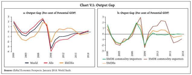 Besides merchandise trade, commercial trade in services also recorded a broad-based recovery across AEs and EMDEs in 2017 after it plunged in 2016 (Chart V.3b). Global information technology spending – a critical driver of global trade in software services – is projected to improve in 2018, though the stricter US policy of issuing H-1B visas could be a potential drag.
V.2 Commodity Prices and Inflation During H2:2017 and Q1:2018, global commodity price movements have largely reflected commodity- specific demand-supply imbalances and the movement of the US dollar. The Bloomberg commodity index increased by 3.6 per cent during October to March 2018. The food price index of the Food and Agriculture Organisation (FAO) fell by 3.2 per cent on account of decline in prices of sugar and dairy products. International sugar prices, in particular, came under considerable downward pressure mostly because of record levels of output in major producing countries, which released substantial export surpluses (Chart V.4a). Crude oil prices surged by around 22 per cent over the last six months with Brent touching a three- year high in January on strong demand riding the improving outlook for global economic activity, especially manufacturing and reduced supplies as cuts in production by OPEC and Russia offset the ramped up shale production in the US. The weak US dollar has also provided a fillip (Chart V.4b). 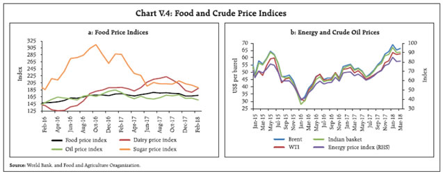 Base metal prices rose by 2.3 per cent during October to March led by copper. Copper prices rose by 3.8 per cent during the same period, touching almost four-year high in December 2017, before losing some steam in recent months on the jump in inventories of refined copper, slowdown in imports by China and the equity market sell-off triggering risk-off sentiment (Chart V.5). Gold prices, which had started rising since mid-December due to the weak US dollar, fell to a two- month low at the beginning of March on the outlook for the US economy turning brighter. However, safe haven demand triggered by fears of a trade war led to firming up of prices. 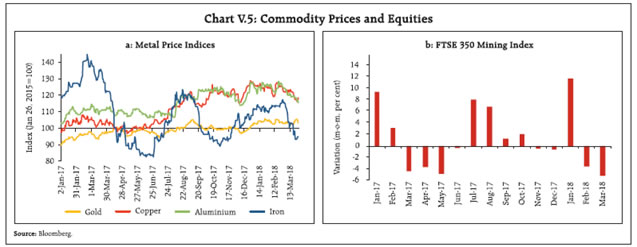 Barring some exceptions, inflation remains subdued and below target levels in major advanced and emerging economies. Among AEs, CPI inflation in the US has risen over the year and has remained above two per cent from October 2017. However, the personal consumption expenditure (PCE) deflator, the measure of inflation used by the Fed, remains below the target. The tightening labour market, rising wages and the boost to disposable incomes from tax cuts pose upside risks. Inflation in the euro area slowed for the third consecutive month in February, despite rising energy prices. In Japan, inflation jumped to a 34-month high in February due to surge in food prices, but remains well below the central bank’s target (Chart V.6a). Inflationary pressures in EMEs are ebbing (Chart V.6b). In Russia, inflation continued to edge lower, falling to a two-decade low in February. In Brazil, inflation moderated on falling housing costs and food prices, while it eased in South Africa to a three-year low in February on falling transport and food costs. China’s consumer price inflation which remained soft until January 2018, rose in February on usual festival related demand. In Indonesia, it has been softening on easing of housing and utility prices. Inflation in Turkey continued to be in double digits, though the easing of price pressures in March pulled it down to an eight-month low. V.3 Monetary Policy Stance The monetary policy stance has remained accommodative in many countries, with the Fed’s policy normalisation progressing along expected lines. The US Fed raised its policy rate by 25 bps each in December 2017 and March 2018 meetings. The March 2018 projections of the Federal Open Market Committee (FOMC) participants suggest that the Fed could hike the policy rate two more times in 2018. In contrast, the ECB has maintained its ultra-accommodative policy stance and kept its rates at a record low. The strong euro is weighing on inflation and keeping it below the target. The Bank of Japan has continued with its ultraaccommodative stance as inflation has remained well below the target (Chart V.7a). Monetary policy stances remained diverse in EMEs, with many central banks in key EMEs reducing policy rates. Central Bank of the Russian Federation cut rates thrice – in December, February and March – with inflation developments remaining favourable, while Brazil has been cutting rates aggressively on underwhelming inflation. South Africa cut its policy rate in March on subsiding inflation. The People’s Bank of China has left its benchmark one-year lending and deposits rates unchanged since October 2015, preferring to influence borrowing costs through liquidity operations and inter-bank market rates. Among other EMEs, Indonesia has kept its policy rate unchanged since the rate cut effected in September 2017. Turkey kept its policy rate unchanged as inflation remained elevated. Mexico raised its policy rate twice in December and March on rising inflation concerns (Chart V.7b). V.4 Global Financial Markets Although markets remained relatively calm and stable during most part of 2017 and January 2018 even in the wake of the unwinding of the Fed’s balance sheet, financial markets turned volatile in February and went into swift correction on fears of faster rate hikes by the US Fed. Early March also witnessed the return of volatility on announcement of protectionist measures by the US and the momentary calm was shattered by intensification of trade protectionism between China and the US. The growing financial market integration in recent years has led to spillovers of volatility from AEs to EMEs due to monetary policy actions and financial events, as witnessed recently (Box V.1). Equity prices have risen across most AEs and EMEs on improving global growth prospects and still accommodative monetary policy stances (Chart V.8a). The Morgan Stanley Capital International (MSCI) World Index increased by 3.9 per cent between October 2017 and March 2018. Equity markets, which had surged during Q4:2017 and January 2018, tanked due to sharp sell-offs across the globe during February on rising interest rate concerns in the US. Just when the equity market in the US began to recover with investors shrugging off fears of inflation worries, volatility returned in March on announcement of US trade policies. In the euro area, equity prices have remained under pressure, lagging behind most peers on expectations of lower corporate earnings and revenue due to a strong euro. Also negotiations surrounding Brexit and election in some member countries adversely impacted investor sentiment. In Japan, a rally in share prices during 2017 and early 2018 was driven by stronger economic performance, higher corporate earnings and lower corporate tax rates. In February, Japanese stock markets cooled during the global stock market sell-off, with the rising yen also slicing away some gains. 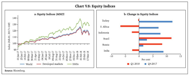
Box V.1: Global Shocks and Spillovers to EMEs – An Episodic Analysis Integration of financial market segments across economies increases the vulnerability of EMEs to geo-political events and shifts in monetary policy stances of systemically important central banks. Over the last decade, many EMEs had to adjust their policies and frameworks to deal with these shocks emanating from advanced economies (AEs). A financial shock originating in a particular country/region can inflate geographically through three possible channels1, viz., portfolio rebalancing, banking liquidity and signalling [Patra et al.(2016)]. An analysis of three episodes of volatility spillovers (Table V.1.1) on the equity, bond and foreign exchange markets in Brazil, India, Russia, South Africa and Turkey using daily data from January 1, 2007 to February 26, 2018 yields interesting results. In this regard, rolling window of six months with reference to pre- and postevent date/period were considered for the episodic analysis. Three proxies for global shocks, viz., US VIX as the ‘fear’ index for equities, broad dollar index (DXY) for the currency market and spread between 10-year and 3-month US treasury yields (term premia) for the bond market were taken as control variables. At the peak of global financial crisis during 2008-2009, markets appeared to have been impacted relatively more by quantitative easing (QE) of AEs. Subsequently, AEs resorted to prolonged QE contingent upon the pace of global economic recovery. Measures taken by EMEs to counter the impact of unconventional policies kept volatility contained, though interspersed by episodes of high turbulence triggered by random events (Chart V.1.1). | Table V.1.1: Major Episodes of Global Spillover | | Episode | Date/period | Impact on EMEs | | Unconventional monetary policies, viz., zero lower bound policy rate and quantitative easing by major AE central banks. | From November 2008 in a phased manner up to October 2014 | Unconventional liquidity injection led to large capital inflows to EMEs resulting in heightened volatility in the equity and forex markets. | | Hints of monetary policy normalisation by the US Fed (taper tantrum). | May 22 – August 10, 2013 | Portfolio outflows from EMEs triggering high volatility in equity, debt and currency markets. | | Unwinding of US Fed balance sheet and reversal of monetary policy stance. | June 20, 2017 onwards | Portfolio rebalancing channel played a dominant role, followed by the liquidity channel by way of portfolio reallocation towards AEs – liquidity conditions in EMEs tightened. |
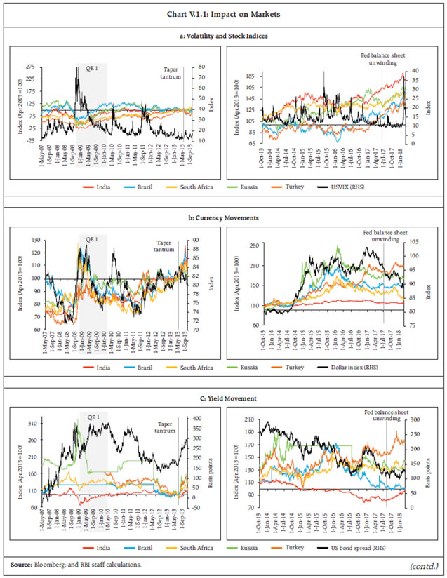 In a Generalised Auto Regressive Conditional Heteroskedasticity (GARCH) framework, the control variables are entrenched in the mean equations for respective markets as follows: where yt denotes the returns on the daily equity indices or currency indices or change in sovereign yields (10-year) in various EMEs; and xt denotes the appropriate control variables (US VIX, DXY and spread between 10-year and 3-month US treasury yields). The variance equation provides the time-varying volatility of the residuals (εt) generated from the mean equation, which consists of three components, viz., long-term average components (w), the last period forecast variance (σ2) and volatility observed in the previous period (ε2). Large values of both α and β suggest increased conditional volatility. While large value of α implies greater response of innovation caused by episodic or unpredictable news/events, large value of β indicates the persistence of volatility. In equity markets, GARCH coefficients (β) were found highly statistically significant across countries during the different phases of QE in the US2. The taper tantrum of 2013 had an impact on all markets due to its suddenness, though South Africa and India were impacted the most. Moreover, balance sheet normalisation had an impact on all EMEs, barring Russia. The news effect (α) was statistically significant for all EMEs, during all the episodes, though Russia remained insulated from the balance sheet normalisation announcement. In currency markets, β was significant in all EMEs during QE1,i.e. November 2008 to March 2010, though the impact of taper tantrum did not persist in Russia. The coefficient α was found to be highly significant among all the EMEs, though the magnitude was larger for Brazil and Turkey during QE1 and for Turkey and Russia during taper tantrum. In the sovereign bond market, β was significant for India and Turkey during all three events. The findings suggest α adversely impacted all sovereign bond markets, though the impact was mostly felt in Brazil and Russia during QE1 and taper tantrum. The above analysis suggests that the three global shocks did cause volatility and adverse reactions across EMEs and across different asset markets, in varying degrees. All the three episodes impacted the bond market more than the currency and the equity segments, with the impact of the taper tantrum being more severe than the other two. References: Apostolou, A., and J. Beirne (2017), “Volatility Spillovers of Federal Reserve and ECB Balance Sheet Expansions to Emerging Market Economies”, ECB Working Paper Series No. 2044. Patra, M. D., S. Pattanaik, J. John and H. K. Behera (2016), “Global Spillovers and Monetary Policy Transmission in India”, RBI Working Paper Series No. 03.
_______________________________________________________________ | Equity markets in EMEs have also gained, notwithstanding the sharp sell-off in February and March, though their performance continued to be dominated by country-specific factors (Chart V.8b). These markets have become volatile in the recent period amidst the repricing of inflation risk, higher US sovereign yields, and more recently, on announcement of protectionist measures by the US Administration. Sovereign bond yields in many AEs hardened with the 10-year US sovereign bond yield touching a four-year high in February on expectations of faster rate hikes by the Fed. Recent inward looking policies have also soured investor sentiment and impacted bond yields adversely. In the euro area, the benchmark 10-year German bond yield has risen, though weak inflation numbers in the euro area have exerted some downward pressure. In Japan, bond yields have been falling since February 2018, coming off from a multi-month high on Japan’s yield curve control policy (Chart V.9a). Bond yields in EMEs were driven by country-specific factors, though they have risen recently in most countries on expectations of shrinking global liquidity and pick-up in inflation in the US. Currency markets have been driven mainly by monetary policy stances in the key AEs and macroeconomic data. The US dollar continued to depreciate and fell to a multi-year low in January on improving growth prospects in other regions. Weaker GDP data for Q4:2017 and comments by authorities in January in favour of a weaker dollar also weighed on the currency. In early March, however, the US dollar rose on upbeat views by the Fed on the US economy, but fell again on fears of intensification of trade wars. The euro is trading at its highest level in more than three years on narrowing of growth differentials between the euro area and its peers and the weakening of the US dollar. The Japanese yen touched the highest level against the US dollar since November 2016 on fears of a trade war. The MSCI Emerging Market Currency index hit a two-month high in January 2018 on the US dollar’s weakness, rising commodity prices and a more synchronised growth upturn, along with ebbing political concerns in some of the constituents (Chart V.9b). Most Asian currencies have retreated in the wake of the recent stock market turmoil, global trade risks and the upbeat US economic outlook, though investors continue to discriminate on countryspecific factors. V.5 Conclusion Global economic activity has been witnessing a broadbased cyclical upturn. The acceleration in global trade outpacing global growth is a welcome development. Inflation remains below policy target levels in many key economies despite rise in some commodity prices and improving demand outlook, while monetary policy stances remain diverse. The recent volatility in financial markets stemming mainly from the uncertainty over the pace of normalisation of monetary policy in AEs could pose a challenge to the EMEs, while fears of rising trade protectionism have clouded the global trade outlook.
ABBREVIATIONS | AEs | Advanced Economies | | AIFIs | All India Financial Institutions | | AQR | Asset Quality Review | | AR(1) | Autoregressive of Order One | | ARCH | Autoregressive Conditional Heteroscedasticity | | AUM | Assets Under Management | | BE | Budget Estimates | | BP | Band-Pass | | bps | Basis Points | | CAD | Current Account Deficit | | CASA | Current Account and Saving Account | | CBLO | Collateralised Borrowing and Lending Obligation | | CCIL | Clearing Corporation of India Ltd. | | CD | Certificate of Deposit | | CDS | Credit Default Swap | | CGST | Central Goods and Services Tax | | CII | Confederation of Indian Industry | | CLI | Composite Leading Indicator | | CMIE | Centre for Monitoring Indian Economy | | CP | Commercial Paper | | CPC | Central Pay Commission | | CPI | Consumer Price Index | | CPI-AL | Consumer Price Index for Agricultural Labourers | | CPI-IW | Consumer Price Index for Industrial Workers | | CPI-RL | Consumer Price Index for Rural Labourers | | CRAR | Capital to Risk Weighted Assets Ratio | | CRR | Cash Reserve Ratio | | CSO | Central Statistics Office | | CU | Capacity Utilisation | | DEA | Digestive Enzymes and Antacids | | DISCOMs | Distribution Companies | | DXY | US Dollar Index | | ECB | European Central Bank | | EMDEs | Emerging Market and Developing Economies | | EMEs | Emerging Market Economies | | ENSO | EI Nino Southern Oscillation | | EU | European Union | | FAE | First Advance Estimate | | FAO | Food and Agriculture Organisation | | FDI | Foreign Direct Investment | | FICCI | Federation of Indian Chambers of Commerce and Industry | | FMCG | Fast-moving Consumer Goods | | FIMMDA | Fixed Income Money Markets and Derivatives Association | | FOMC | Federal Open Market Committee | | FPI | Foreign Portfolio Investment/Investor | | FRBM | Fiscal Responsibility and Budget Management | | FTSE | Financial Times Stock Exchange | | FY | Financial Year | | GARCH | Generalised Autoregressive Conditional Heteroscedasticity | | GDP | Gross Domestic Product | | GFCE | Government Final Consumption Expenditure | | GFCF | Gross Fixed Capital Formation | | GFD | Gross Fiscal Deficit | | GMM | Generalised Method of Moments | | GNDI | Gross National Disposable Income | | G-Secs | Government Securities | | GST | Goods and Services Tax | | GVA | Gross Value Added | | GSDP | Gross State Domestic Product | | H1 | First Half of the Year | | H2 | Second Half of the Year | | HNI | High networth individual | | HRA | House Rent Allowance | | IBC | Insolvency and Bankruptcy Code | | IIP | Index of Industrial Production | | IMD | India Meteorological Department | | IMF | International Monetary Fund | | IPO | Initial Public Offering | | LAF | Liquidity Adjustment Facility | | LIBOR | London Interbank Offered Rate | | LIC | Life Insurance Corporation of India | | LPG | Liquefied Petroleum Gas | | LTCG | Long Term Capital Gain | | M3 | Broad Money | | MCLR | Marginal Cost of Funds Based Lending Rate | | MEP | Minimum Export Price | | MFs | Mutual Funds | | MMTC | Metals and Minerals Trading Corporation of India | | MNREGA | Mahatma Gandhi National Rural Employment Guarantee Act | | m-o-m/M-o-M | Month-on-Month | | MPC | Monetary Policy Committee | | MPR | Monetary Policy Report | | MSCI | Morgan Stanley Capital International | | MSF | Marginal Standing Facility | | MSP | Minimum Support Price | | MSS | Market Stabilisation Scheme | | NAFED | National Agricultural Cooperative Marketing Federation of India | | NBER | National Bureau of Economic Research | | NBFCs | Non-Banking Financial Companies | | NCAER | National Council of Applied Economic Research | | NDTL | Net Demand and Time Liabilities | | NEER | Nominal Effective Exchange Rate | | NFC | Non-Food Credit | | NGNF | Non-Government Non-Financial | | NHB | National Housing Bank | | NIM | Net Interest Margin | | NPA | Non-performing Asset | | NRI | Non-Resident Indian | | NSDL | National Securities Depository Limited | | NSE | National Stock Exchange | | NSSF | National Small Savings Fund | | OECD | Organisation for Economic Co-operation and Development | | OG | Output Gap | | OIS | Overnight Index Swap | | OMCs | Oil Marketing Companies | | OMOs | Open Market Operations | | OPEC | Organization of the Petroleum Exporting Countries | | PADO | Public Administration, Defence and Other services | | PCE | Personal Consumption Expenditure | | PFCE | Private Final Consumption Expenditure | | PMI | Purchasing Managers’ Index | | PSU | Public Sector Undertaking | | QE | Quantitative Easing | | q-o-q/Q-o-Q | Quarter-on-Quarter | | RBI | Reserve Bank of India | | RE | Revenue Expenditure/Revised Estimate | | REER | Real Effective Exchange Rate | | RERA | Real Estate (Regulation and Development) Act | | RHS | Right Hand Side | | RRBs | Regional Rural Banks | | SAAR | Seasonally Adjusted Annualised Rate | | SAE | Second Advance Estimates | | SCBs | Scheduled Commercial Banks | | SDF | Standing Deposit Facility | | SDLs | State Development Loans | | SEBI | Securities and Exchange Board of India | | SFAC | Small Farmers’ Agri-Business Consortium | | SLR | Statutory Liquidity Ratio | | SME | Small and Medium Enterprise | | SPD | Standalone Primary Dealer | | T-Bill | Treasury Bill | | UDAY | Ujwal DISCOM Assurance Yojana | | UK | United Kingdom | | US | United States | | VAR | Vector Autoregression | | VIX | Volatility Index | | WACR | Weighted Average Call Money Rate | | WADTDR | Weighted Average Domestic Term Deposit Rate | | WALR | Weighted Average Lending Rate | | WPI | Wholesale Price Index | | WTI | West Texas Intermediate | | WTO | World Trade Organization | | y-o-y/Y-o-Y | Year-on-Year | |