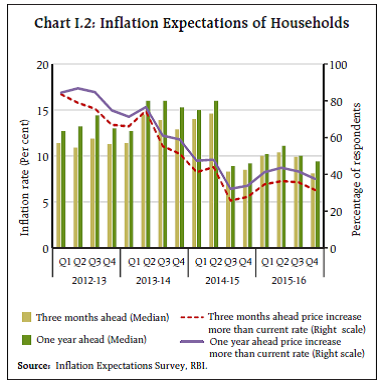
| I. Macroeconomic Outlook Headline CPI inflation is projected to moderate in 2016-17 to around 5 per cent while real GDP growth is projected to improve gradually to 7.6 per cent in 2016-17. Heightened global financial market volatility continues to pose major risks to these projections. Two landmark developments in the period since the September 2015 Monetary Policy Report (MPR) will fundamentally shape the institutional architecture of monetary policy in India. First, the inflation target of 6 per cent for January 2016 set for itself by the Reserve Bank and subsequently adopted formally under the Monetary Policy Framework Agreement (MPFA) was achieved. With inflation targets having been met consecutively since January 2015, it entrenches credibility in the commitment to the flexible inflation targeting (FIT) framework. Inflation is currently within the 4 ± 2 per cent band adopted for FIT. The path to the mid-point of the band will, however, be calibrated so that the output effects of disinflation are smoothed. Accordingly, the next milestone is set at 5 per cent for inflation by the end of 2016-17. Second, in his speech presenting the Union Budget for 2016- 17, the Union Finance Minister announced that the Reserve Bank of India Act is being amended to provide statutory basis for a monetary policy framework and a monetary policy committee (MPC) (Chapter XII of the Finance Bill provides specific features of the proposal). Committee-based decision making will mark a watershed in the historical evolution of monetary policy in India. As stated by the Finance Minister, it is expected to add value and transparency to the monetary policy decisions. As the processes leading up to the functioning of the MPC are set in motion, they will bring in their train significant changes in institutional design and greater accountability. Domestically, the macroeconomic situation has evolved broadly in line with the September baseline scenario, with real gross value added (GVA) growth and inflation trajectories moving in alignment with staff’s forecasts. Chapters II and III describe forecasts and outcomes. Two developments warrant a re-assessment of forecasts (Chart I.1). First, the significant softening of crude oil prices since November 2015 together with the signals in futures prices suggest a lower crude oil price for 2016-17 in this MPR’s baseline scenario (Table I.1). Secondly, prospects for external demand for 2016 are now weaker than envisaged six months back, with downside risks amplified by the worsening macroeconomic outlook and tighter financial conditions for emerging market economies (EMEs). Overall, global risks have increased significantly. I.1 Outlook for Inflation Inflation expectations of households, corporations and financial market participants are largely adaptive in their formation. Consequently, most recent inflation developments, and particularly those relating to salient items in consumption baskets, tend to influence these expectations. The January-March 2016 round of the Reserve Bank’s inflation expectations survey of urban households indicates some softening of inflation perceptions and expectations1. The decline in current perceptions and three months ahead expectations - by almost 2 percentage points below the results for the previous round - was more pronounced than in one year ahead expectations (0.6 percentage points). Both current perceptions (7.9 per cent) and three months ahead expectations (8.1 per cent) in the March 2016 round were the lowest since September 2009. Nevertheless, one year ahead inflation expectations (9.4 per cent) continue to show hysteresis and various expectations measures rule above actual inflation. The proportion of respondents expecting prices to rise by more than the current rate fell in the March 2016 round (Chart I.2). | Table I.1: Baseline Assumptions for Near-Term Projections | | Variable | September 2015 MPR | Current (April 2016) MPR | | Crude Oil (Indian Basket)* | US$ 50 per barrel in H2:2015-16 | US$ 40 per barrel during FY 2016-17 | | Exchange rate ** | ₹ 66/US$ (the then prevailing level) | Current level | | Monsoon | 86 per cent of long- period average (LPA) in 2015 | Normal for 2016 | | Global growth *** | 3.3 per cent in 2015 3.8 per cent in 2016 | 3.4 per cent in 2016 3.6 per cent in 2017 | | Fiscal deficit | To remain within BE 2015-16 (3.9 per cent) | To remain within BE 2016-17 (3.5 per cent) | | Domestic macroeconomic/ structural policies | No major change | No major change | Note:
*: Represents a derived basket comprising sour grade (Oman and Dubai average) and sweet grade (Brent) crude oil processed in Indian refineries in the ratio of 72:28.
**: The exchange rate path assumed here is for the purpose of generating staff’s baseline growth and inflation projections and does not indicate any ‘view’ on the level of the exchange rate. The Reserve Bank is guided by the need to contain volatility in the foreign exchange market and not by any specific level/ band around the exchange rate.
***: Based on projections in the July 2015 and January 2016 updates of the IMF’s World Economic Outlook. |
 In the March 2016 round of the Nikkei’s manufacturing purchasing managers’ survey, input costs and factory gate prices picked up. On the other hand, the January- March 2016 round of the Reserve Bank’s industrial outlook survey points to expectations of stable output prices on the back of softer cost conditions (Chart I.3). Growth in staff costs in the organised sector, both manufacturing and services, decelerated during 2015- 16:Q3. The Reserve Bank’s industrial outlook survey suggests some salary pressures going forward. Rural wage growth exhibited moderation in 2015-16:Q4. Professional forecasters (March 2016 round of the survey) expect inflation to remain around 5.2-5.3 per cent during 2016-17. Their medium- and long-run expectations (5 years and 10 years ahead, respectively) were 5.0 per cent and 4.8 per cent, respectively (Chart I.4). These poll results may be indicative of the anchoring of inflation expectations around the Reserve Bank’s inflation target. Information on the final target of monetary policy, i.e., inflation, is typically lagged and provisional when it arrives. The central bank’s own forecast, however, contains all the information relevant to the outlook for inflation, including the policymaker’s preferences regarding the short-run trade-off between output and inflation as well as the estimated effects of shocks working their way through the economy. This inflation forecast, therefore, provides an ideal intermediate target for monetary policy, mirroring the behaviour of the final target over the relevant policy horizon. Inflation forecast targeting frameworks have helped in containing inflation and anchoring inflation expectations in both advanced and emerging market economies. Importantly, they have also been associated with a lowering of the variability of inflation outcomes. The experiences of Canada (an advanced economy) and Czech Republic (an emerging economy) attest to these gains (Chart I.5). Enhanced credibility in the Reserve Bank’s commitment to its inflation objective can play an important role in the transmission of monetary policy responses to inflation and output shocks (Box I.1). 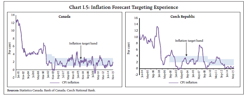 Incorporating signals from various indicators and revisions in assumptions on initial conditions into updated estimates of structural models yields a projection path in which headline CPI inflation decelerates modestly to 5.3 per cent in Q1 of 2016-17, and then abates to 5.1 per cent in Q2, 5.0 per cent in Q3 and 5.1 per cent in Q4. The 2016-17:Q4 projections are placed in a 70 per cent confidence interval of 3.2 per cent to 7.7 per cent (Chart I.6). Assuming a normal monsoon, further fiscal consolidation in line with the path set out in the Union Budget and no major exogenous or policy shocks, model estimates indicate that CPI inflation would moderate to 4.2 per cent in Q4 of 2017-18, with risks tilted to the upside. The implementation of one-rank-one-pension (OROP) for retired defence employees and the 7th Central Pay Commission (CPC) award, particularly with regard to house rent allowances, poses upward risks to the baseline inflation path, especially as state governments also start implementation. Box I.1: Central Bank Credibility and Monetary Policy Dynamics A monetary policy framework with a commitment to low and stable inflation warrants as a pre-condition that the central bank strengthens its credibility by achieving inflation targets, while recognising and communicating short-run trade-offs. Since January 2014, headline CPI inflation in India has moved broadly in line with the Reserve Bank’s disinflation glide path and more recently, inflation expectations in the economy have started to moderate in reflection of gains in the Reserve Bank’s credibility. Optimal monetary policy responses have been calibrated under three alternative credibility scenarios in a model with India specific features - low credibility (0.25); moderate credibility (0.675); and perfect credibility (1.0). Under the low credibility scenario, the central bank has to raise the policy rate aggressively to create slack in the economy for achieving disinflation (Chart). The sacrifice ratio (the cumulative foregone annual output for each percentage point of inflation decline) is about 2.0. At the other end is the perfect credibility scenario in which the public has full confidence in the framework. The disinflation announcement by the central bank itself reduces inflation expectations. Lower expected inflation raises the real interest rate, without any need for an increase in the nominal rate (in fact, in the model, the nominal rate declines with a lag). This opens up a marginal negative output gap and the sacrifice ratio is only about 0.5. In the intermediate case of moderate credibility stock, the nominal interest rate needs to increase, although not as aggressively as in the low credibility case, so as to induce the necessary slack in the economy, with a sacrifice ratio of around 1.25. 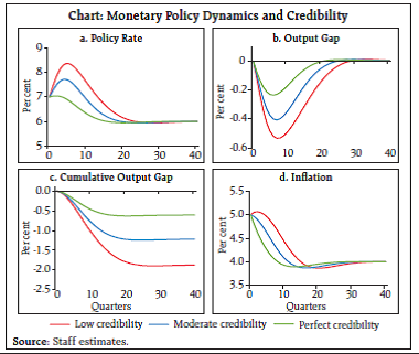 References: Alichi, A., H. Chen, K. Clinton, C. Freedman, M. Johnson, O. Kamenik, T. Kisinbay, and D. Laxton (2009). “Inflation Targeting under Imperfect Policy Credibility”, IMF Working Paper, No. 09/94. Benes, J., K. Clinton, A. George, J. John, O. Kamenik, D. Laxton, P. Mitra, G.V. Nadhanael, H. Wang and F. Zhang (2016). “Inflation Forecast Targeting for India: An Outline of the Analytical Framework” (Mimeo). I.2 Outlook for Growth A number of factors could impinge upon the growth outlook for 2016-17. First, slow investment recovery amidst balance sheet adjustments of corporates is likely to hinder investment demand. Secondly, with capacity utilisation in the organised industrial sector estimated at 72.5 per cent, revival of private investment is expected to be hesitant. Thirdly, global output and trade growth remain tepid, dragging down net exports. On the positive side, the government’s “start-up” initiative, strong commitment to fiscal targets, and the thrust on boosting infrastructure could brighten the investment climate. Household consumption demand is expected to benefit from the Pay Commission award, continued low commodity prices, past interest rate cuts, and measures announced in the Union Budget 2016-17 to transform the rural sector. Consumer confidence remains upbeat, as polled in the March 2016 round of the Reserve Bank’s survey, with optimism on prospects for income and economic conditions (Chart I.7). A similar improvement is visible in the MNI India Consumer Sentiment survey, with households optimistic about the purchasing environment. The corporate sector’s expectations of business conditions dipped but remained positive according to the Reserve Bank’s industrial outlook survey (Chart I.8). Surveys conducted by other agencies indicate a mixed picture (Table I.2). Professional forecasters surveyed by the Reserve Bank during March 2016 expected output growth to pick up gradually from 7.3 per cent in 2015-16:Q4 to 7.7 per cent in 2016-17:Q4, almost entirely on account of recovery in agriculture and allied activities (Chart I.9 and Table I.3). Staff projects GVA growth to improve gradually during 2016-17 to 7.6 per cent, with quarterly growth in a range of 7.3-7.7 per cent and risks evenly balanced around this baseline projection (Chart I.10). These estimates incorporate revisions in assumptions on initial conditions, structural model estimates and off model adjustments prompted by lead and coincident indicators of economic activity, results from forward-looking surveys, and an assessment of the impact of the 7th CPC and the Union Budget. For 2017-18, real growth in GVA is projected at 7.9 per cent, assuming a normal monsoon, continued boost to consumption from the Pay Commission award and no policy induced structural change or any major supply shock. | Table I.2: Business Expectations Surveys | | | NCAER Business Confidence Index | FICCI Overall Business Confidence Index | Dun and Bradstreet Composite Business Optimism Index | CII Business Confidence Index | | Q3: 2015-16 (January 2016) | Q3: 2015-16 (January- February 2016) | Q1: 2016 (December 2015) | Q3: 2015-16 (January 2016) | | Current level of the index | 130.3 | 56.7 | 85.9 | 53.9 | | Index as per previous Survey | 129.5 | 64.1 | 79.3 | 53.4 | | % change (q-o-q) sequential | 0.6 | -11.5 | 8.4 | 0.9 | | % change (y-o-y) | -12.2 | -19.6 | 2.5 | -4.1 |
I.3 Balance of Risks The baseline projections of growth and inflation are subject to several risks. Plausible alternate scenarios in which some of the risks, both downside and upside, materialise are presented below. 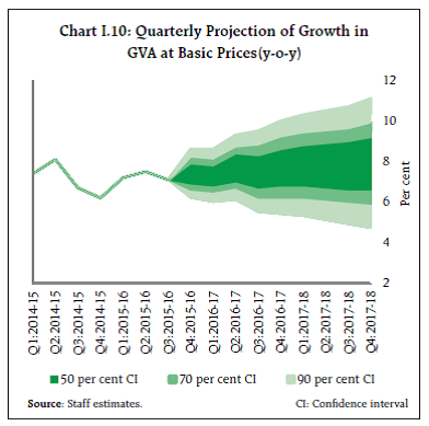
| Table I.3: Reserve Bank's Baseline and Professional Forecasters' Projections | | (Per cent) | | | 2015-16 | 2016-17 | 2017-18 | | Reserve Bank’s Baseline Projections | | | | | Inflation, Q4 (y-o-y) | 5.4 | 5.1 | 4.2 | | Real Gross Value Added (GVA) Growth | 7.3 | 7.6 | 7.9 | | Assessment of Survey of Professional Forecasters @ | | | | | GVA Growth | 7.3 | 7.7 | | | Agriculture and Allied Activities | 1.1 | 2.6 | | | Industry | 7.5 | 7.4 | | | Services | 9.0 | 9.1 | | | Gross Domestic Saving (per cent of GNDI) | 30.7 | 30.8 | | | Gross Fixed Capital Formation (per cent of GDP) | 29.4 | 30.0 | | | Money Supply (M3) Growth | 11.6 | 12.7 | | | Bank Credit of Scheduled Commercial Banks Growth | 11.4 | 12.3 | | | Combined Gross Fiscal Deficit (per cent of GDP) | 6.5 | 6.2 | | | Central Government Gross Fiscal Deficit (per cent of GDP) | 3.9 | 3.5 | | | Repo Rate (end period) | 6.75 | 6.25 | | | CRR (end period) | 4.00 | 4.00 | | | Yield of 91-days Treasury Bills (end period) | 7.2 | 6.8 | | | Yield of 10-years Central Government Securities (end period) | 7.6 | 7.4 | | | Overall Balance of Payments (US $ bn.) | 24.7 | 35.0 | | | Merchandise Exports Growth | -16.2 | 1.7 | | | Merchandise Imports Growth | -13.5 | 4.4 | | | Merchandise Trade Balance (per cent of GDP) | -6.3 | -6.4 | | | Current Account Balance (per cent of GDP) | -1.0 | -1.3 | | | Capital Account Balance (per cent of GDP) | 2.2 | 2.9 | | @: Median forecasts. GNDI: Gross National Disposable Income.
Source: 39th Round of Survey of Professional Forecasters (March 2016) | (i) Implementation of the Seventh Pay Commission Award The implementation of the CPC’s recommendations could impact inflation and growth through: a) the direct impact of the proposed increase in the house rent allowance (HRA); b) indirect effects operating through consumption to aggregate demand; and c) inflation expectations channel (see Chapter 2). With propagation to states, there is likely to be an amplification of the total impact on the housing inflation component and hence on overall CPI. The impact is expected to persist up to 24 months. Assuming that the Government implements the Commission’s recommendations by the second quarter of 2016-17, CPI inflation could be, on average, 100-150 bps higher than the baseline in 2016-17 and 2017-18 (Chart I.11). Of course, the Government’s decision on implementation of the 7th CPC is still awaited. (ii) Weaker Global Growth Recent developments point towards a weakening of global economic activity. If it materialises, unsettled financial markets could generate spillovers to the broader global economy. A widening of the slack in the global economy by 1 percentage point over the baseline will result in growth in India turning out to be 20-40 bps below the baseline (Chart I.12). Inflation would also be lower by 10-20 bps as lower demand would result in a fall in global commodity prices. (iii) Exchange Rate While the macroeconomic fundamentals of Indian economy remain strong, volatility in the foreign exchange market on account of external developments can impact both growth and inflation trajectories. A 5 per cent depreciation relative to the baseline assumption could lead to inflation turning up by 10- 15 bps above the baseline forecast for 2016-17 and real GVA growth by around 5-10 bps above the baseline. (iv) Deficient Monsoon El Nino conditions continue to pose a risk to the south-west monsoon. About 90 per cent of all El Nino years have led to below normal rainfall and 65 per cent of El Nino years have brought droughts. Assuming a deficiency of 20 per cent in the monsoon, lower agriculture output could lower the overall GVA growth by around 40 bps in 2016-17. Food prices could consequently increase, leading to inflation rising above the baseline by 80-100 bps in 2016-17, even assuming effective government policies relating to food stocks, procurement and minimum support prices (MSPs). (v) Rise in Crude Oil Prices There is considerable amount of uncertainty on oil prices in view of political forces impacting oil market dynamics. Supply disruptions from geo-political developments could lead to spikes in oil prices, while weaker global demand could push prices further down. If oil prices rise to around US$50 per barrel, and assuming full pass-through to domestic fuel prices, inflation could be higher by 40-60 bps and growth could be weaker by 20-30 bps. On the other hand, a reduction in crude oil prices to around US$ 20 per barrel could reduce inflation by 80-120 bps, while boosting real GVA growth by 40-60 bps. Sustained disinflation is beginning to have a moderating impact on inflationary expectations. Along with the favourable baseline outlook on crude oil and other commodity prices, and a still negative output gap, inflation is expected to remain inertial but quiescent over 2016-17 and 2017-18. Deviations of the south-west monsoon from normal, upside shocks to oil prices and weak growth in a number of advanced and emerging economies would pose downside risks to the baseline projections of growth and inflation set out in this MPR.
II. Prices and Costs Consumer price inflation rose in the second half of 2015-16 before dropping in February with a sharp decline in food prices. Farm and non-farm cost pressures abated and wage growth in rural areas as well as in the organised sector remained weak. The September 2015 MPR projected headline CPI inflation1 to rise from 4.5 per cent in that month to an average of 5.5 per cent in Q3 and 5.8 per cent in Q4 of 2015-16. Actual inflation outcomes have closely followed this projected trajectory, and especially the turning points, albeit with a marginal undershoot that has become somewhat pronounced in February 2016 (Chart II.1). Factors that explain the slightly softer than projected inflation readings are: (i) cereal inflation remaining contained by astute supply management; (ii) softening of crude oil prices from December onwards to below US$ 30 per barrel in January 2016, a 12-year low; and (iii) sharp fall in vegetable prices since December 2015. In January, headline inflation was 5.7 per cent, within the disinflation target of 6 per cent set for January 2016. A sharper than anticipated seasonal moderation in vegetable prices took inflation down to 5.2 per cent in February. These developments have considerably bolstered the likelihood that the target of 5 per cent set for 2016-17 will be achieved. II.1 Consumer Prices Favourable base effects, which had nudged inflation into a dip during July-August 2015, waned from September and consequently, inflation rose for six months successively before subsiding in February (Chart II.2). This period was marked by persisting momentum in month-on-month (m-o-m) price changes during September-November. Although m-o-m price changes turned negative in December, the impact on overall inflation was overwhelmed by a large unfavourable base in that month. By February, the momentum of inflation declined and reinforced the favourable base effect (Chart II.3). Some food groups, especially pulses, have given the distribution of inflation a high positive skew (Chart II.4). Even as inflation ebbs, its persistence remains unchanged reflecting the stickiness in prices of pulses and several categories of services (Chart II.5). A diffusion index2, measuring the tendency of the bulk of prices to move in one direction, shows that for overall CPI as well as constituent goods and services, readings were much above 50 per cent in Q3 and Q4, indicating broad-based price increases. In February, the diffusion index for goods fell, while for services it moved up sharply to close to the 100 per cent mark (Chart II.6). II.2 Drivers of Inflation In 2015-16 so far, services inflation remained sticky, with its average contribution during April-February slightly higher (25.5 per cent) than its weight (23.4) in overall CPI. The contribution of consumer durables to overall inflation has also remained steady (Chart II.7). The category of food and beverages contributed 53 per cent to the average headline inflation (5.4 per cent). Food inflation rose unrelentingly from September 2015 to January 2016 in a broad-based manner to an intra year peak before easing in February. With inflation in cereals, fruits and animal based proteins remaining range-bound, the price behaviour of pulses and vegetables largely determined the food inflation trajectory in this period (Chart II.8). Pulses alone contributed to over 35 per cent of food inflation despite a low share of about 5 per cent within the food and beverages group (Chart II.9). The recurrence of high pulses inflation reflects the structural gap in availability relative to demand. India is the largest producer and consumer of pulses, with cross-border trade accounting for barely 15 per cent of India’s annual production. The focus of agricultural research needs to shift urgently to pulses with emphasis on developing short-duration pest- and disease-resistant varieties, seed multiplication and measures to boost crop yield so as to start off India’s second green revolution. 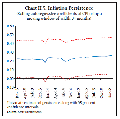 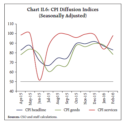 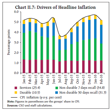 Vegetables inflation also edged up during November 2015-January 2016 as unseasonal rains and flood in southern states limited the extent of price decline usually seen in winter months. However, as the crop arrival picked up, vegetables prices fell sharply in February, pulling down overall food inflation. In other food items, price pressures were visible in the case of sugar as global prices increased in anticipation of a shortfall in production. Pressures remained persistent within the protein-rich category, especially meat and fish for which supply has not been able to match up the increasing demand. 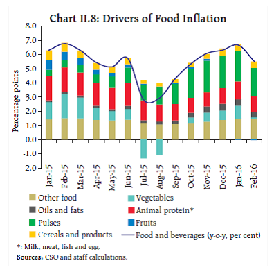 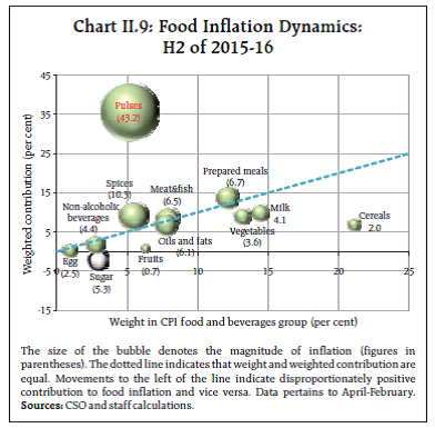 Cereals and products constitute 21.1 per cent of the CPI food basket. Their prices have risen only marginally, despite a second successive year of deficient monsoon. A range of measures were taken by the Government, including lower order of increases in minimum support prices (MSPs) and higher off-take by states to moderate price pressures. Furthermore, there has been a secular fall in world cereals prices since 2013 leading to a 45 per cent correction in global prices from their peaks. Other factors include slowdown in rural wage growth and falling input costs. In the fuel group, inflation remained steady since September but fell sharply in February (Chart II.10). International prices for kerosene and liquefied petroleum gas (LPG) remained muted and the gap with respect to domestic administered prices of kerosene and LPG closed over the course of the financial year. Electricity inflation decelerated after December. Firewood, with the second largest weight in the fuel group, continued to remain the major inflation driver in the category. CPI inflation excluding food and fuel edged up gradually from 4.3 per cent in August 2015 to 4.9 per cent in February 2016, largely on account of higher inflation in the sub-groups of transport and communication, and housing. Adjusted for petrol and diesel components of transportation, however, inflation in this category remained sticky with only a modest softening in Q4 print (Chart II.11). Petrol and diesel prices exhibited a slower rate of deflation from Q3 than in preceding quarters. This was on account of sequential increase in excise duty rates in petrol and diesel since November 2015 (Chart II.12). The cumulative increase in petrol and diesel excise duties by around ₹ 12 per litre and ₹ 14 per litre, respectively, since November 2014 had a direct impact of around 90 basis points on CPI inflation excluding food and fuel and around 40 basis points on headline inflation. Furthermore, in March both petrol and diesel prices increased following the increase in global crude prices. Housing inflation rose gradually and continuously since September. Going forward, the forthcoming implementation of the 7th Central Pay Commission (CPC) recommendations could significantly alter the trajectory of overall inflation over the medium-term (Box II.1). Other measures of inflation Exclusion based measures of CPI inflation remained sticky due to the impact of non-tradable items in the CPI basket (Chart II.13). Trimmed mean measures of CPI inflation, on the other hand, softened in Q4 and remained below headline inflation. Empirical evidence suggests that food and fuel inflation affects headline inflation in India3 through formation of high inflation expectations, wage increases and rise in other commodity prices. The spill-over from food to non-food inflation is found to be stronger during healthy domestic demand conditions4. Understanding the shocks in food and fuel prices and their spillovers could provide meaningful insights for monetary policy in anchoring inflation expectations. Inflation measured by other consumer price indices moved synchronously with headline CPI inflation. The deflation in WPI appears to have bottomed out in Q2 of 2015-16. GVA and GDP deflators that were in negative terrain in Q2, turned positive in Q3. The gap between CPI and WPI started narrowing in Q4 so far (Table II.1). Box II.1: Implication of Central Pay Commission Awards on the Medium-term Inflation Trajectory The implementation of the 7th Central Pay Commission (CPC) awards can have a significant bearing on the inflation trajectory through both direct and indirect channels. In case of subsidised housing provided by the Government, rent charged for the dwelling is the house rent allowance (HRA) normally admissible to the employee along with a nominal license fee. An increase in HRA leads to an increase in imputed rent for Government provided accommodation. Such HRA awards, by their construct, seek to bring parity of housing allowances by the Government with the prevailing market rates. Thus, the direct effect on inflation comes through a higher housing index. The indirect effects stem from an increase in private consumption expenditures and through second-round increases in rental rates for housing in general which could embed higher inflation expectations in the public’s perception. The 6th CPC awards were implemented in August 2008 with HRA awards coming into effect from September 2008. On account of the methodology of collecting rental data in CPI-IW1, the direct impact occurred with a lag during July 2009-January 2010 when the contribution of housing to overall inflation stood in excess of 25 per cent (Chart a). The direct impact of the 6th CPC awards on CPI-IW inflation was estimated at 2.5 percentage points in July 2009, which rose to around 4 percentage points by January 2010. Most of the Statewise housing indices showed significant increases by July 2010, indicating quick follow-through of CPC increases to States (Table). As a result of the staggered increase in State Government employees’ HRA, the rate of increase in housing index remained high till January 2012. 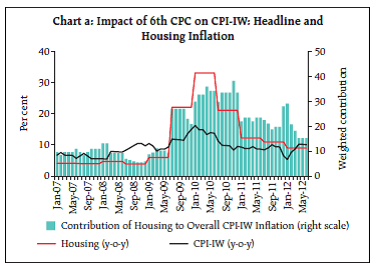
| Table: M-o-M Increase (per cent) in CPI-IW Housing During 6 CPC: Select States | | Sr. | State | Jan-09 | Jul-09 | Jan-10 | Jul-10 | Jan-11 | Jul-11 | Jan-12 | | 1 | Andhra Pradesh | 4.8 | 13.5 | 12.4 | 5.4 | 6.3 | 5.3 | 3.2 | | 2 | Assam | 1.6 | 5.1 | 4.4 | 1.2 | 1.6 | 9.3 | 5.4 | | 3 | Bihar | 2.0 | 23.5 | 22.2 | 6.1 | 5.3 | 4.7 | 1.9 | | 4 | Gujarat | 2.7 | 15.2 | 13.0 | 6.1 | 6.5 | 7.6 | 3.5 | | 5 | Haryana | 3.7 | 15.3 | 16.0 | 8.1 | 5.0 | 3.1 | 1.9 | | 6 | Karnataka | 7.6 | 12.9 | 9.7 | 2.5 | 2.4 | 2.4 | 3.1 | | 7 | Kerala | 4.5 | 14.9 | 8.1 | 1.9 | 2.8 | 4.1 | 2.5 | | 8 | Madhya Pradesh | 2.3 | 17.2 | 20.5 | 6.5 | 5.3 | 2.5 | 2.6 | | 9 | Maharashtra | 3.2 | 12.0 | 9.5 | 10.0 | 11.2 | 5.8 | 2.9 | | 10 | Odisha | 6.2 | 36.5 | 17.0 | 8.3 | 7.8 | 6.0 | 2.0 | | 11 | Punjab | 6.3 | 18.9 | 12.7 | 4.7 | 4.0 | 3.1 | 2.1 | | 12 | Rajasthan | 3.9 | 16.3 | 16.4 | 3.6 | 2.1 | 6.5 | 1.9 | | 13 | Tamil Nadu | 4.8 | 10.7 | 8.0 | 6.2 | 2.0 | 1.6 | 2.4 | | 14 | Uttar Pradesh | 7.0 | 29.4 | 21.9 | 5.5 | 3.5 | 3.2 | 2.4 | | 15 | West Bengal | 3.5 | 15.0 | 12.0 | 4.4 | 7.9 | 8.7 | 6.6 | The indirect impact of the 6th CPC award on overall CPI-IW inflation worked out to around 60 basis points based on estimates derived from vector autoregression (VAR) and structural models. The direct impact of the 7th CPC recommendations on headline inflation is expected to be around 150 basis points. The indirect effects are estimated to be around 40 basis points. The impact of the pay awards is likely to be seen over a period of two years (Chapter 1). Compared to the 6th CPC awards, increase in the housing index would be more quick and continuous2 and indirect effects are likely to be smaller. Moreover, outgo of arrears under 7th CPC awards would be substantially lower but HRA rates would automatically increase when the dearness allowance of the employees crosses threshold levels3.
II.3 Costs Since the MPR of September 2015, cost pressures in the economy have abated with the sustained fall in global energy and non-energy prices. Domestic input cost pressures also remained subdued. Both industrial and farm costs remained in contractionary mode, albeit with some pick-up in sequential terms in recent months (Chart II.14). In the farm sector, electricity, fertiliser and agricultural machinery prices remained rangebound whereas diesel prices moderated. In case of the non-farm sector, decline in minerals prices and fall in fuel prices provided comfort. Wholesale input price inflation closely tracks the assessment of manufacturing firms participating in the Reserve Bank’s industrial outlook survey. The 73rd round of the survey conducted in January-March 2016 reports moderation in input price growth, with the softness in costs extending into the near-term. This sentiment was driven by companies that are benefiting from the fall in international commodity prices, especially those in the petroleum and metal industries. Declining wholesale price inflation attested to the moderation in the cost of raw materials. Falling input prices and weak demand conditions kept corporate pricing power in check. In case of the services sector, however, increase in input costs was reported across all major sectors such as hotels and restaurants, finance, and transport companies. | Table II.1: Measures of Inflation | | (Y-o-y, per cent) | | Quarter/ Month | GVA Deflator | GDP Deflator | WPI | CPI | CPI- IW | CPI- AL | CPI- RL | | Q1 : 2014-15 | 7.2 | 5.9 | 5.8 | 7.4 | 6.9 | 8.1 | 8.3 | | Q2 : 2014-15 | 2.1 | 1.8 | 3.9 | 6.7 | 6.8 | 7.3 | 7.6 | | Q3 : 2014-15 | 2.9 | 3.5 | 0.3 | 4.1 | 5.0 | 5.4 | 5.7 | | Q4 : 2014-15 | 1.0 | 2.3 | -1.8 | 5.3 | 6.6 | 5.8 | 6.0 | | Q1 : 2015-16 | 0.0 | 1.0 | -2.3 | 5.1 | 5.9 | 4.4 | 4.7 | | Q2 : 2015-16 | -2.1 | -1.2 | -4.6 | 3.9 | 4.6 | 3.1 | 3.4 | | Q3 : 2015-16 | 0.7 | 1.8 | -2.3 | 5.3 | 6.5 | 5.0 | 5.2 | | Jan-16 | | | -0.9 | 5.7 | 5.9 | 5.6 | 5.7 | | Feb-16 | | | -0.9 | 5.2 | 5.5 | 5.0 | 5.3 | | IW: Industrial Workers, AL: Agricultural Labourers and RL: Rural Labourers. | Rural wages, a key determinant of farm costs, recorded moderate growth in nominal terms and remained almost stagnant in real terms (Chart II.15). Part of the moderation in nominal wage growth could be in response to the fall in inflation. Wage growth in the organised sector, reflected in per employee cost, decelerated in Q3 of 2015-16 for both manufacturing and services, with the manufacturing sector registering a sharper decline. While wage growth in manufacturing sector slowed down, value of production in manufacturing sector decelerated at a much faster pace leading to an increase in unit labour cost (as measured by ratio of staff cost to value of production, Chart II.16). Understanding price setting behaviour in an economy is important for monetary policy, especially in gauging rigidities in price formation which generate welfare losses (Blinder et al. (1998)5, Loupias (2013)6, Dias et al. (2015)7). A random effects ordered probit model on the panel of companies covered in the Reserve Bank’s industrial outlook survey from 2010-20148, suggests that raw material costs, labour costs and cost of finance influence price setting behaviour with a decreasing order of impact. Pricing decisions generally vary based on company size, seasonality, past price changes as well as in the way firms adjust to shocks. Firms respond more often in response to a price shock by adjusting prices upwards than in the other direction. Similarly, strong demand conditions induce higher increase in prices, whereas the likelihood of lowering the price in case demand is weak is lower. This suggests that the response of expansionary and contractionary monetary policies in controlling inflation will also be asymmetric – expansionary policy fuels inflation at a rate faster than contractionary policy can contain it9. 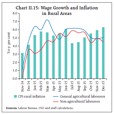 New forms of transactions such as online exchange and e-commerce are gaining currency in India, especially in the urban areas. The cost of adjustments in prices may be limited in such forms of transactions and, therefore, price rigidities induced by menu costs may turn out to be less relevant. Also, prices could turn out to be extremely flexible with dynamic pricing models and strategies adopted by such firms. These developments complicate the setting of monetary policy as the prices of such items are not currently covered in the official price statistics.
III. Demand and Output Domestic activity slowed in the second half of 2015-16. Aggregate demand was restrained by stalling fixed investment, weak rural consumption and the ongoing fiscal consolidation. Aggregate supply moderated with the impact of deficient monsoons on agriculture. Gross value added in industry benefited from the decline in input costs while services remained in expansion mode. Domestic economic activity lost pace in the second half of 2015-16, slowed down by muted investment and a prolonged contraction in exports. While private consumption has been the mainstay in holding up aggregate demand, it has largely been an urban phenomenon; coincident indicators of rural consumption have generally remained weak or in negative territory. On the supply side though, some silver linings are discernible. Despite consecutive deficient monsoons and unseasonal weather more recently, foodgrains production is on course to post a modest improvement over the levels recorded a year ago. For industry, the deceleration in the volume of production has been more than offset by the decline in input costs. While service sector activity has been affected by the subdued performance of tradables, non-tradables have been expanding at a reasonable pace. III.1. Aggregate Demand Aggregate demand in terms of year-on-year (y-o-y) changes in real gross domestic product (GDP) at market prices moderated in the second half of 2015-16, encountering headwinds from stalling fixed investment (Table III.1). | Table III.1: Real GDP Growth | | (Per cent) | | Item | Weighted Contribution* | 2014-15 | 2015-16 (AE) | 2014-15 | 2015-16 | | 2014-15 | 2015-16 (AE) | Q1 | Q2 | Q3 | Q4 | Q1 | Q2 | Q3 | Q4# | | I. Private Consumption Expenditure | 3.5 | 4.2 | 6.2 | 7.6 | 8.2 | 9.2 | 1.5 | 6.6 | 6.4 | 5.6 | 6.4 | 11.7 | | II. Government Consumption Expenditure | 1.3 | 0.3 | 12.8 | 3.3 | 9.0 | 15.4 | 33.2 | -3.3 | 1.0 | 4.3 | 4.7 | 3.0 | | III. Gross Fixed Capital Formation | 1.6 | 1.7 | 4.9 | 5.3 | 8.3 | 2.2 | 3.7 | 5.4 | 5.2 | 7.6 | 2.8 | 5.5 | | IV. Net Exports | 0.2 | 0.1 | 11.7 | 6.1 | 62.8 | -72.5 | -111.1 | -6.6 | -7.6 | -6.5 | 30.4 | 16.6 | | (i) Exports | 0.4 | -1.5 | 1.7 | -6.3 | 11.6 | 1.1 | 2.0 | -6.3 | -5.8 | -4.3 | -9.4 | -5.7 | | (ii) Imports | 0.2 | -1.6 | 0.8 | -6.3 | -0.6 | 4.6 | 5.7 | -6.1 | -5.0 | -3.4 | -10.8 | -6.0 | | V. GDP at Market Prices | 7.2 | 7.6 | 7.2 | 7.6 | 7.5 | 8.3 | 6.6 | 6.7 | 7.6 | 7.7 | 7.3 | 7.7 | AE: Advance estimates.
*: Component-wise contributions to growth do not add up to GDP growth in the table because change in stocks, valuables and discrepancies are not included.
#: Implicit growth rate calculated from AE of 2015-16.
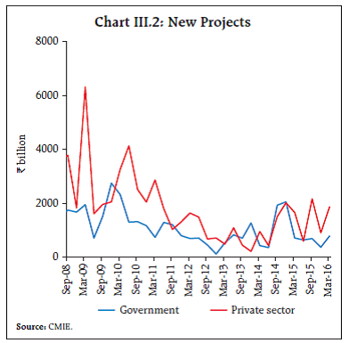
Source: Central Statistics Office (CSO). | The stock of stranded investment in stalled projects fell, reflecting concerted efforts by the Government towards fast-tracking the revival of projects in electricity generation and chemicals sectors (Chart III.1). New investment remained subdued in both private and public sectors in response to the prevailing uncertainty in the business environment and muted business confidence (Chart III.2). The production of capital goods fell sharply, co-moving with a deceleration in imports, barring in February (Chart III.3). A durable recovery in the capex cycle continues to remain elusive in the face of considerable slack. Profitability of the non-government non-financial companies has also moderated in Q3, with implications for corporate saving and investment. These coincident indicators suggest that national accounts data for Q4 of 2015-16, especially private final consumption expenditure (PFCE), may be subject to downward revisions from the implicit levels in the advance estimates for the full year. 
 PFCE expanded in H2, in part benefiting from real income gains from lower average inflation than a year ago. The production of consumer durables rose robustly up to January 2016, also reflecting improvement in credit conditions for consumers as banks rebalanced their lending portfolios in favour of personal loans in which stress is relatively low. Sales of commercial and passenger vehicles, production of gems and jewellery and mixers and grinders accelerated, indicative of the resilience of urban consumption. Purchasing managers’ surveys point to some improvement in employment in manufacturing industries. 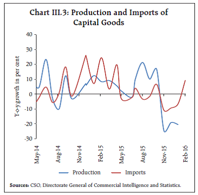 By contrast, rural consumption remained weak in H2; with moderation in wage growth, rural incomes have been depressed by shocks to farm activity from back-to-back deficient monsoons. In Q4, however, there was a pick-up in sales of tractors and two-wheelers which could be indicative of a turning point in the rural economy (Chart III.4). The focus of the Union Budget 2016-17 on reviving the rural economy and doubling rural incomes could support rural consumption demand more enduringly going forward. Overall, the prospects for PFCE have been brightened by the proposal to implement the 7th Pay Commission award and one-rank-one-pension for retired defence personnel. The growth of government final consumption picked up in H2 relative to H1. The Centre’s revenue expenditure rose on higher spending on major subsidies, especially petroleum subsidies, and higher interest payments. Plan revenue expenditure related to social and physical infrastructure made a turnaround in H2 from an absolute decline in H1. Capital expenditure of the Centre decelerated in H2 in relation to H1, reflecting lower growth in capital outlay. States, accounting for nearly two-third of general government capital expenditure, received significantly higher resources on account of their enhanced share in taxes as recommended by the Fourteenth Finance Commission. The expenditure multiplier of States tends to be higher than that of the Centre, which could work towards reviving overall investment in the economy. 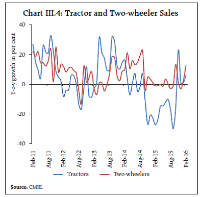 For the year as a whole, the revised estimates indicate that growth in aggregate expenditure of the Central Government was higher than a year ago with revenue and capital expenditure broadly in line with their respective budgetary targets. Despite a large shortfall vis-à-vis projected disinvestment, the buoyancy in indirect tax collections and non-tax revenues helped in meeting the fiscal deficit target (Table III.2). The combined fiscal deficit at 6.5 per cent of GDP in 2015-16 is budgeted to have improved in relation to a year ago at 7 per cent. The Union Budget 2016-17 adhered to the path of fiscal consolidation with the Centre’s gross fiscal deficit (GFD) projected to decline by 0.4 percentage points. Adherence to fiscal consolidation path is contingent upon efficient revenue mobilisation - broadening the tax base and rationalising exemptions reflect the Government’s intent in this direction. The stance of fiscal policy in 2016-17 will face a challenging trade-off sustaining public investment within the straitjacket of shrinking fiscal headroom (Chart III 5). | Table III.2: Key Fiscal Indicators-Central Government Finances | | Indicators | As per cent of GDP | | 2015-16 (BE) | 2015-16 (RE) | 2016-17 (BE) | | 1. Revenue Receipts | 8.1 | 8.9 | 9.1 | | a. Tax Revenue (Net) | 6.5 | 7.0 | 7.0 | | b. Non-Tax Revenue | 1.6 | 1.9 | 2.1 | | 2. Total Non-Debt Receipts | 8.7 | 9.2 | 9.6 | | 3. Non-Plan Expenditure | 9.3 | 9.6 | 9.5 | | a. On Revenue Account | 8.5 | 8.9 | 8.8 | | b. On Capital Account | 0.8 | 0.7 | 0.7 | | 4. Plan Expenditure | 3.3 | 3.5 | 3.7 | | a. On Revenue Account | 2.3 | 2.5 | 2.7 | | b. On Capital Account | 1.0 | 1.0 | 1.0 | | 5. Total Expenditure | 12.6 | 13.2 | 13.1 | | 6. Gross Fiscal Deficit | 3.9 | 3.9 | 3.5 | | 7. Revenue Deficit | 2.8 | 2.5 | 2.3 | | 8. Primary Deficit | 0.7 | 0.7 | 0.3 | | Memo: Additional resource mobilisation for infrastructure financing* (₹ billion ) | ... | 400 | 313 | BE: Budget estimates. RE: Revised estimates.
*: Includes bonds allocated to NHAI, IRFC, HUDCO, IREDA, PFC, REC and NTPC for 2015-16 and NHAI, PFC, REC, IREDA, NABARD and Inland Water Authority for 2016-17.
Source: Union Budget 2016-17. | Net exports turned positive in Q3 for the first time in the year and contributed modestly to the increase in aggregate demand in the quarter. The contraction in merchandise exports, which began in December 2014 and peaked in Q3 of 2015-16 was primarily on account of weakening global demand and the persistent fall in international commodity prices. World trade volume was pulled down by a deepening contraction in demand from emerging market economies (EMEs) – which absorb more than half of India’s exports. POL (petroleum, oil and lubricants) exports declined by more than 50 per cent, mainly attributable to the decline in international crude prices, although export volumes also shrank. Similarly, non-POL exports also contracted in nominal terms, and the highly adverse international environment drove the volume of these exports into negative territory, as in Q2. Merchandise imports recorded a precipitous decline in Q3, mainly on account of POL and gold. Even excluding these items, imports declined by about 9 per cent. The merchandise trade deficit was lower than in preceding quarters and was mainly responsible for the improvement in net exports in the national accounts, since net exports of services remained broadly stable. India continued to benefit from an improvement in the terms of trade, with import prices falling faster than those of exports. 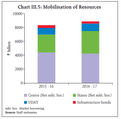 In Q4, exports remained in contraction mode in January and February 2016 across both POL and non-POL products. Exports have declined in nominal terms for fifteen successive months; however, the contraction eased to a single digit on a y-o-y basis. Powering the turnaround were gems and jewellery, drugs and pharmaceuticals, electronics and chemicals. The decline in imports also slowed. While POL imports fell on account of further softening of crude oil prices, gold imports also declined in anticipation of lower import duties in the Union Budget 2016-17. An important development in Q4 was the resumption of positive growth in non-oil non-gold imports in February after a gap of seven months, largely contributed by imports of machinery, pearls, precious stones, and electronic goods. The trade deficit narrowed sharply in January and February 2016 reflecting these developments. India’s share in world exports has declined from its recent peak of 1.7 per cent in 2014 to 1.6 per cent even as some major advanced economies (AEs) and peer Emerging Market and Developing Economies (EMDEs) gained share (Chart III.6). This suggests that factors such as the rising incidence of protectionism and competitive depreciation might have affected export performance, since depressed global demand is common to all exporting countries. 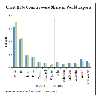 Financing of net exports in Q3 of 2015-16 mainly took the form of foreign direct investment (FDI) which, at US$ 14 billion was the highest ever quarterly net inflow of FDI to India. Foreign portfolio investment, by contrast, recorded net outflows in H2 as heightened turbulence in global financial markets triggered shifts in investors’ risk appetite and flights to safe haven. In March, however, FPIs returned as risk-on sentiments took hold. Other forms of capital inflows, however, remained subdued in Q3. There was an accretion to foreign exchange reserves, taking their level to US$ 355.6 billion as on March 25, 2016, equivalent to about 10 months of imports. III.2. Aggregate Supply The rate of growth in output measured by gross value added (GVA) at basic prices moderated in H2 of 2015-16 on a y-o-y basis (Table III.3). In terms of seasonally adjusted quarter-on-quarter (q-o-q) annualised growth, the loss of momentum was even more stark (Chart III.7). Actual quarterly outcomes have closely adhered to the projection path given in the September MPR, with small deviations in magnitude around the turning points. In Q2, the upturn in construction turned out to be more moderate than initially anticipated. The magnitude of recovery in corporate earnings was also somewhat muted. Real GVA growth slowed between Q2 and Q3 in line with projections, but it was 10 basis points above the projection, with manufacturing value added surprising on the upside (Chart III.8). 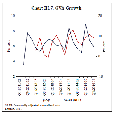
| Table III.3 Sector-wise Growth in GVA | | (Per cent) | | Sector | 2014-15 | 2015-16 | 2015-16 | | Q1 | Q2 | Q3 | Q4# | | I. Agriculture and Allied Activities | -0.2 | 1.1 | 1.6 | 2.0 | -1.0 | 2.6 | | II. Industry | 6.5 | 8.8 | 7.1 | 8.4 | 11.0 | 8.7 | | Manufacturing | 5.5 | 9.5 | 7.3 | 9.0 | 12.6 | 9.4 | | III. Services | 9.4 | 8.4 | 8.5 | 8.3 | 8.6 | 8.2 | | Construction | 4.4 | 3.7 | 6.0 | 1.2 | 4.0 | 3.5 | | Trade, Hotels, Transport, Communication | 9.8 | 9.5 | 10.5 | 8.1 | 10.1 | 9.3 | | Financial, Real Estate & Professional Services | 10.6 | 10.3 | 9.3 | 11.6 | 9.9 | 10.1 | | GVA at Basic Prices | 7.1 | 7.3 | 7.2 | 7.5 | 7.1 | 7.4 | #: Implicit growth rate calculated from AE of 2015-16.
Source: CSO. | Value added in agriculture and allied activities contracted in Q3 and dragged down overall GVA growth in the quarter. After the south-west monsoon ending the season with a deficit of 14 per cent relative to the long period average (LPA), the north-east monsoon started on a listless note with a highly skewed spatial distribution entailing risks to soil moisture. Sowing of major rabi crops except coarse cereals was significantly below normal. An important buffer was the foodgrains stock which remained higher than the new norms through the year. In the first part of November, Tamil Nadu, which receives almost half of its rainfall from these rains, was buffeted by cyclonic weather and excess precipitation. Floods adversely affected coffee plantations and paddy sowing. The shortfall in the production of pulses - arhar and urad - became binding in the context of the spike in prices of pulses. The north-east monsoon ended in December with a deficiency of 23 per cent of the LPA, particularly acute in central, western and parts of eastern India. In Q4, rabi sowing improved in January mainly on account of return of rain and chill in the north and north-eastern parts of the country. 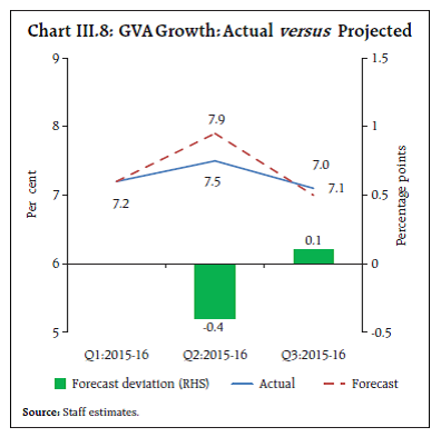 In the context of crop losses in 2015-16 due to vagaries of weather, the Fasal Bima Yojana announced on January 13, 2016 assumes importance. It envisages a uniform premium of 2 per cent to be paid by farmers for all kharif crops and 1.5 per cent for all rabi crops. In case of annual commercial and horticultural crops, the premium to be paid by farmers will be 5 per cent. The balance premium will be paid by the Government to provide full insurance to farmers against crop loss on account of natural calamities. Remote sensing and smart phones technologies will be used to fast track the payment of claims. In February, the second advance estimates placed foodgrains output at 0.5 per cent higher in 2015-16 than the previous year. This positive outcome reflects the impact of greater weather proofing of Indian agriculture and timely intervention by the government over a wide area, including pre-emptive advisories, contingency plans and promotion of better variety seeds. In recent years, the horticulture sector has been imparting resilience to overall agriculture performance. Growth in production of horticulture crops (5.3 per cent) outstripped the production of foodgrains (1.6 per cent) in terms of the 12-year average (Chart III.9). Although forecasts for the south-west monsoon 2016 are not yet available from the IMD, the chance of El Niño gradually decreases into the spring and turns neutral by May-June-July 2016, according to the US National Oceanic Atmospheric Administration. The chance of La Niña increases to 50 per cent in September- October-November 2016. In the Indian context, some of the strongest El Niño years have been followed by La Niña episodes, resulting in bumper harvests1. Value added in the industrial sector accelerated in H2 of 2015-16, led by manufacturing. By contrast, industrial output measured by the Index of Industrial Production (IIP) could not sustain the base-effect surge in October and fell into contraction through January 2016. Soft commodity prices brought down input costs sharply as well as the implicit GVA deflator for industry, which together explains the wedge between value added and IIP (Chart III.10). In terms of use-based activity, all segments suffered output losses, except festival related demand for consumer durables and intermediate goods in H2. The contraction in industrial output was not, however, broad-based - excluding 2 per cent on either side on account of volatile items, the IIP rose by 0.9 per cent; excluding capital goods, the rest of IIP expanded by 1.4 per cent in December 2015. In Q4, the IIP continued to contract for the third successive month during January 2016, again mainly led by decline in manufacturing. Electricity generation remained resilient and is expected to sustain its performance backed by thermal supplies, while consumer durables continued to gain from favourable base effects. The sharp contraction in capital goods was primarily due to the decline in production of cables and insulated rubber; excluding this lumpy item the IIP would have shown a modest increase of 1.7 per cent. Consumer non-durables continued to shrink in the absence of support from demand. Consequently, the overall consumer goods sector stayed flat, while basic goods decelerated. The manufacturing PMI for March 2016 expanded on the basis of growth of output, new orders, including exports. The Make in India drive, together with new measures announced in the Union Budget to widen the space for FDI, and custom and excise concessions, are expected to help lift industrial performance. In this context, the start-up India initiative assumes importance as a potential game changer in lifting business sentiment. The objective is to create an ecosystem that is conducive for entrepreneurship, employment generation and wealth creation. Gross value added in the services sector maintained a stable pace of expansion in H2, as it had in the first half of 2015-16. All constituents shared in this growth, although financial services, real estate and professional services experienced some moderation. 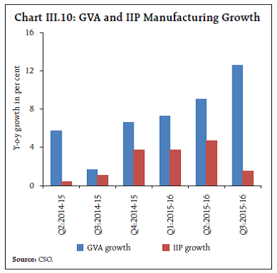 In Q3, the services PMI was in expansionary territory in October on new business orders, but it fell to a five month low in November as new business orders slowed down (Chart III.11). In December, the index surged back but polled firms indicated a reluctance to hire. Other lead and coincident indicators of service sector activity were mixed and reflected sector-specific dynamics. By October through the quarter, passenger and commercial vehicles sales registered healthy growth on festival related demand and one-time replacement requirements to comply with fuel emission norms. On the other hand, the two wheelers segment remained subdued compared to other segments as rural demand remained moribund. Steel consumption and cement production – compositely, a lead indicator of construction activity – anticipated a slowdown in an environment of legacy issues especially delays in clearances and land acquisition, weak demand and unsold inventory. The revival in roads and highways construction and commercial real estate activity cushioned the downturn. In the trade sector, port traffic decelerated. In Q4, the services PMI remained in expansion zone but dipped sequentially, unable to sustain the smart improvement in January 2016. The moderation occurred on account of softer growth in new business. Other indicators moved diversely. Sales of commercial vehicles showed an uptick in January, while passenger vehicles sales decelerated to lowest in seven months possibly because of correction in inventory management and ban in the national capital region (NCR) on registration of diesel vehicles with higher engine capacity. Sales of passenger vehicles continued to remain subdued in February 2016 exacerbated by strikes in Haryana affecting supplies while commercial vehicles sales continue to accelerate. Overall freight traffic and particularly in respect of coal, the largest commodity carried by railways, contracted during February 2016. Port cargo was, however, boosted by higher tonnage of POL and containerised cargo. III.3. Potential Output Revisited Potential output generally refers to the level of output that is consistent with low and stable inflation. Divergence between the levels of actual output and potential output and expressed as a proportion of potential output, i.e. the output gap, indicates excess demand when it is positive, leading to inflationary pressures. There is now a wide consensus that potential output across the world has been lastingly impaired since or even before the global financial crisis2. By how much should current estimates of potential output be lowered is, however, unclear since these estimates tend to be highly sensitive to the choice of data/sample period and methodology. Nonetheless, misperceptions of the current output gap could lead to notably higher inflation in the near term, and sharply lower growth and increasing external imbalances in the case of delay in recognising the error (IMF, 2011)3. The output gap in India was positive during Q1 of 2005-06 through Q1 of 2012-13 except in Q4 of 2008-09, and turned negative since Q2 of 2012-13 with the downturn in the business cycle; it was (-)0.6 per cent in Q3 of 2015-16. The derived rate of growth of potential output was around 5 per cent during 1981-1991, increasing to around 6 per cent during 1992-2002 and to 8 per cent during 2003-2008. It has, however, fallen in the post global crisis period to around 7 per cent during 2009-2015 (Box III.1). Box III.1: Alternative Approaches to Estimating Potential Output Methods for estimating potential output can be broadly categorised into three groups: (i) purely statistical methods (e.g. time trend estimation; statistical filters), (ii) methods that combine structural relationships with statistical methods (e.g., the Kalman filter) and (iii) structural methods which are based on economic theory (e.g., the production function approach). Each methodology has limitations which influence the estimate of potential output and appropriate caveats are warranted in the interpretation of results4. Against this backdrop, a pragmatic approach is to estimate potential output employing a battery of statistical and structural methods on quarterly GVA data (Q2:1980 – Q4;2015)5 and then to combine these results using principal component analysis to produce composite estimates of the output gap. This estimate closely co-moves with inflation excluding food and fuel and capacity utilisation – two indicators of aggregate demand conditions – attesting to the robustness of the estimation (Chart a & b). 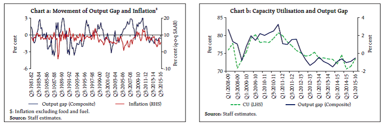 Reference: Bhoi, B.K. and H.K. Behera (2016), “India’s Potential Output Revisited’’, RBI Working Papers (forthcoming). The recent deceleration in India’s potential growth is attributed largely to slowdown in investment and a modest decline in total factor productivity. Hence, key to acceleration of India’s growth lies in augmentation of capital formation and raising the productivity of labour and capital so as to be able to operate the economy at the technology possibility frontier.
IV. Financial Markets and Liquidity Conditions Money, bond and credit markets have been largely insulated from global spillovers, while foreign exchange and equity markets have experienced bouts of volatility. Liquidity conditions generally tightened in the second half of the year and proactive liquidity management alleviated pressure on money market rates. Long-term yields exhibited a tightening bias till February and risk spreads reflected both corporate sector stress and asset quality concerns in banks. Total flow of resources to the corporate sector remained buoyant, with industry receiving a rising proportion of increase in non-food credit. With the turn of the year, global financial markets were seized with renewed fears of a weakening global economy. Volatility surged, dispelling the calm in the preceding quarter that had enabled a priced-in response to the start of normalisation of the US monetary policy in December. As the final section of this chapter shows, financial markets in India exhibited differentiated responses to these developments. Money, bond and credit markets have been largely insulated from global developments. By contrast, foreign exchange and equity markets experienced bouts of volatility and were vulnerable to rapid shifts in risk assessments. IV.1 Financial Markets Money markets experienced distinct two-way movements through Q3 of 2015-16. Overnight rates traded with a softening bias in the first half of October, having fully transmitted the end-September policy rate reduction of 50 basis points (bps) amidst easing liquidity conditions. Other short-term rates moved synchronously, with interest rates on both commercial papers (CPs) and 91-day treasury bills (TBs) declining by about 38 bps in response to the repo rate cut. From the second half of October, however, redemption pressures in the equity market due to selling by foreign portfolio investors (FPIs) constrained lending by mutual funds in the collateralised borrowing and lending obligation (CBLO) market and liquidity pressures spread to other segments of the overnight spectrum. The slowing pace of Government expenditure and the onset of festival-related currency demand also contributed to tighter liquidity conditions. Barring brief respites in the early part of each month due to salaries/pension spending by the Government and some return of currency to the banking system after the festivals in late November, the weighted average call rate (WACR) generally remained a little above the repo rate through the quarter - especially around the outflow of advance tax payments in mid-December. Money market rates hardened in Q4 as the spending restraint by the Government became pronounced by mid-January and cash balances began to build-up well ahead of the Union Budget. Term premia rose as secondary market three month CP and certificate of deposit (CD) rates inched up (Chart IV.1). Another factor squeezing liquidity through the quarter was the firming up of non-food credit offtake that started in December. Liquidity tightness was exacerbated from the second week of February, imparting an upside to the WACR. On March 31, the WACR spiked with the Government’s cash balances rising to ₹1.9 trillion and banks building excess reserves of 23 per cent above the requirement. 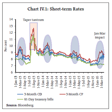 Two factors are notable in recent money market activity. First, asymmetry in the intra-day evolution of the WACR reflects the market microstructure. Money market rates are generally higher during the first hour of trading, reflecting reversal of the previous day’s borrowings as also funding requirements for the day ahead (Chart IV.2). Market activity again picks up during the last hour of trading on reassessment of liquidity positions by banks to meet reserve requirements and other cash flows. The first and last hour of trading covers about 70-75 per cent of daily call market volumes. Secondly, the heightening of liquidity pressures towards the close of Q4 is a recurring phenomenon every year as market participants rush for liquidity for balance sheet adjustments and to meet year-end targets. Cash balances with the Reserve Bank become a preferred asset at this time of the year. With the unwinding of these cash balances, liquidity conditions ease significantly in early April, again a recurring phenomenon year after year. 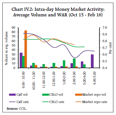 In the bond market, yields on government securities (G-secs) – which had started to ease ahead of the monetary policy easing cycle – got increasingly disconnected and firmed up through the second half of 2015-16. After the announcement of the Union Budget, however, yields steadily eased (Chart IV.3). From the second week of October, the benchmark yield traded with a hardening bias, mainly due to higher primary treasury issuances in October, an uptick in inflation and the depreciation of the rupee brought on by portfolio investment sales. Barring high intensity global events that prompted sell-offs globally, domestic factors have played a predominant role in driving up yields. A rolling regression of India’s 10-year G-sec yield on the US 10-year treasury yield suggests that the sensitivity of domestic yields to global yields has subsided significantly in the recent period1 (Chart IV.4). 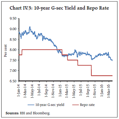 In Q4 of 2015-16, G-sec yields traded with an upward bias. Successive increases in monthly inflation readings, uncertainty on the likely fiscal stance in the Union Budget and concerns about compliance with the liquidity coverage ratio (LCR) norm weighed on yield movements. The introduction of the new 10-year benchmark security on January 11, an OMO purchase auction of ₹ 100 billion on January 20 and the increase in the investment limit for FPIs in the debt segment improved sentiment in the bond market, but it was transient and yields started hardening by the third week of January 2016 right up to the last week of February, due to likely over-supply of papers relative to demand – State Development Loans (SDLs), tax free bonds and Ujwal DISCOM Assurance Yojana (UDAY) bonds. 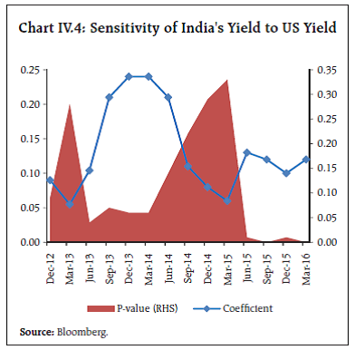 Positive sentiment generated by the Union Budget softened yields, with 10-year generic yield declining by about 16 bps on February 29. G-sec yields edged up in the first half of March on profit-booking by market participants, but traded with a softening bias in the second half on the lower inflation reading for February and dovish guidance by the Fed. High rated corporate bond yields had eased in the early part of Q3, fully pricing in the September policy rate cut. In Q4, however, a hardening bias set in, but eased during the second half of March. Lower rated corporate bond yields rose on concerns related to balance sheets and rising incidence of restructuring of corporate debt by Indian banks (Chart IV.5). The overall corporate stress ratio – the number of rating upgrades divided by the number of downgrades – declined sharply, indicating deterioration of credit quality of Indian firms. Overall, corporate bond spreads widened though the issuance of corporate bonds (public issues and private placements) increased significantly during the year. Equity markets began Q3 on a buoyant note, lifted by the policy rate cut on September 29 which boosted rate-sensitive sectors. With positive global cues, including signals of additional accommodation by the ECB and the Fed holding rates steady, the sensex was supported by the resumption of portfolio flows while domestic institutional investors, including mutual funds, engaged in profit-booking. Towards the end of October, however, indications of monetary policy normalisation in the FOMC’s December meeting, weak quarterly earnings of some domestic blue chip companies and caution ahead of Bihar elections triggered a fresh slide on the domestic bourses. Bearish sentiment persisted through December, with pessimism building on the slow pace of structural reforms, higher CPI inflation readings, slowdown in industrial production, disappointing Chinese economic data and terror attacks in Europe. 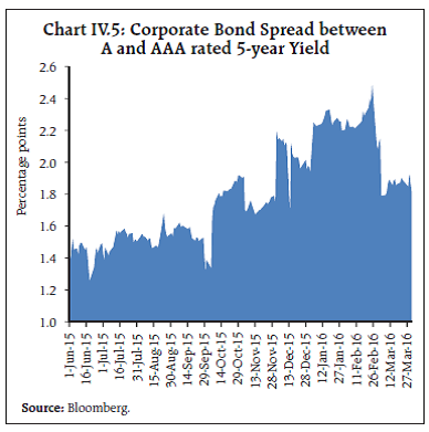 At the start of Q4, global spillovers pulled down the sensex. A slump in oil prices to below US$ 30 per barrel – a 12-year low – and dismal Chinese data coupled with another devaluation of the renminbi triggered a massive retrenchment of portfolio investment across EMEs. Equity markets in India were also affected by weaker than expected corporate earnings forecasts and the depreciation of the rupee. In February, there was a resurgence of stress in global financial markets, triggered by a meltdown in stock markets in China. As spillovers spread, investors questioned the ability of highly leveraged European banks to service their contingent convertible bonds. In India, global risk aversion was amplified by public sector banks declaring steep fall/increase in their net profits/losses in Q3 due to higher provisioning for non-performing assets (NPA) and as a result, banking stocks witnessed a sharp fall in market valuation. The sensex dropped by 22 per cent from its January 2015 highs to a 21-month low and erasing all gains since May 2014. The sensex surged a day after the Union Budget with a return of portfolio flows, improvement in business sentiment and recovery in the rupee amidst strong cues from Asian and European equity markets after China’s central bank cut the reserve requirement ratio. The sensex continued gaining in the following days with heavy buying by foreign investors, surge in banking stocks after core capital requirement rules were eased, appreciation of the rupee and rallies in Asian equity markets on expectations of further stimulus from the ECB. Compared with the secondary market, the initial public offering (IPO) market remained upbeat, recording a four year high mobilisation in 2015 with 64 IPOs aggregating to about US$ 2.2 billion (about ₹ 139 billion). While the IPO index generated return of 19 per cent in 2015, the benchmark sensex yielded a negative return of 5.0 per cent in 2015 (Chart IV.6). 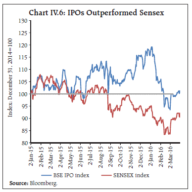 The rupee traded with an appreciating bias against the US dollar in the first half of October, buoyed by the weakness in the US dollar on deferment of monetary policy normalisation in the FOMC’s September 17-18 policy meeting (Chart IV.7a). From mid-October, however, the rupee started to depreciate with the strengthening of the US dollar on increasing market expectations of an increase in the Federal Funds rate in December. Bunching of importers’ demand for foreign currency and risk-averse FPI outflows also imparted downward pressures to the rupee (Chart IV.7b). Barring intermittent gains on profit-taking and positive domestic cues, including better than expected GDP data for Q2, narrowing of the merchandise trade deficit and expansion of the space for FDI, the rupee continued to depreciate through November and December. The December lift-off of the Federal Funds rate turned out to be fully factored in by markets. Dovish Fed guidance brought back stability in foreign exchange markets across EMEs, and the rupee appreciated towards the close of the quarter. 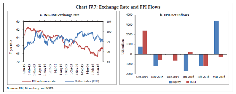 The onset of Q4 brought with it a dramatic shift in the foreign exchange market. Global spillovers produced a renewed bout of downward pressure from the beginning of 2016 as risk aversion and flight to safety intensified on pervasive bearish sentiment. Domestic developments such as rise in inflation, weaker industrial production and continued portfolio outflows also imparted downside to the rupee. The decision of the Bank of Japan to push interest rate into negative territory accentuated the risk-on sentiment towards EMEs in general, resulting in a modest appreciation of the rupee relative to the extent of firming up of several EME currencies (Chart IV.8). Following the announcement of the Union Budget, the rupee appreciated. Since mid-March, the return of portfolio flows to equity market has sustained the upside in the foreign exchange market. In terms of both nominal effective exchange rate (NEER) and real effective exchange rate (REER), the rupee depreciated during 2015-16 by 4.1 per cent and 1.4 per cent, respectively, partly offsetting the appreciation in 2014- 15 (Table IV.1). 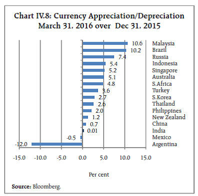 Credit market activity was weighed down by weak demand due to sluggish industrial and corporate activity and the presence of considerable slack. In addition, risk aversion among banks emanating from asset quality concerns restrained credit flows. Non-food bank credit, which had slipped into an extended single-digit growth trough in the first half of 2015-16, picked up in the second half of the year and recorded y-o-y growth rates of 10.7 per cent and 11.3 per cent, respectively, in Q3 and Q4. The upturn is discernible even after adjusting for the operations of Bandhan and IDFC Bank – two new private banks that commenced activity during the year (Chart IV.9a). Noteworthy in this pick-up was that the flow of credit to industry, which had declined in the first half, turned around and accounted for 29 per cent of the total increase in non-food credit in Q3, followed by a share of 34 per cent in Q4 (Chart IV.9b). By and large, the improvement in bank credit flows has been led by the personal loans category, especially housing, in which delinquency and collateral constraints are comparatively less binding. The flow of resources from banks and non-banks to the commercial sector increased by 25 per cent in 2015-16. Flows from non-banks, which include CPs, public issues, financing from all India financial institutions, housing finance companies as well as foreign sources, increased by 12 per cent. 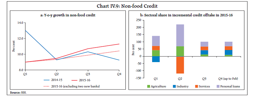
| Table IV.1 : Nominal and Real Effective Exchange Rates: Trade-Based (Base: 2004-05=100) | | Item | Index March 25, 2016 (P) | Appreciation (+) / Depreciation (-) (per cent) | | Mar 2016 over Mar 2015 | Mar 2015 over Mar 2014 | | 36-currency REER | 111.62 | -1.4 | 9.0 | | 36-currency NEER | 73.67 | -4.1 | 6.8 | | 6-currency REER | 122.13 | -3.0 | 11.7 | | 6-currency NEER | 66.43 | -6.7 | 7.1 | | ₹/ US$ (As on Mar 31, 2016) | 66.33 | -5.6 | -4.0 | P: Provisional.
Note: REER figures are based on Consumer Price Index (Combined).
Source: Reserve Bank of India. | In response to the cumulative reduction in the policy repo rate by 125 bps, the weighted average lending rate (WALR) on fresh rupee loans declined by 90 bps (up to February 2016) and even the WALR on outstanding rupee loans softened by 53 bps (Table IV.2). The median base rate of banks, however, declined by 60 bps as against a higher decline of 80 bps in their median term deposit rates during the same period, reflecting the preference of banks to protect profitability in the wake of deteriorating asset quality and higher provisioning. The Marginal Cost of Funds Based Lending Rate (MCLR) system, effective April 1, 2016, is expected to impart greater transparency in the pricing of credit and improve the transmission of policy rate into the lending rates. As on April 4, the median overnight MCLR of 26 banks, accounting for about 83 per cent of total bank credit, was 50 bps lower than the median base rate, while the median MCLR across all tenors was lower by 25 bps. The Government’s decision to remove the spread of 25 bps on select small savings schemes vis-a- vis G-sec yields of comparable maturities, and introduce a more frequent (quarterly, instead of annual) resetting of the administered interest rates on all small savings schemes effective Q1 of 2016-17 should align small savings rates with market rates and contribute to strengthening transmission. Administered interest rates on small savings schemes have been marked down by 40-130 bps for Q1 of 2016-17 as compared with those for 2015-16. In Q3 of 2015-16, the Reserve Bank started the Asset Quality Review (AQR) to ensure that banks were taking proactive steps to correctly classify their loan portfolios, with the deadline of March 2017 to clean up by making full provision. Fifteen public sector banks reported losses on their domestic operations in Q3 of 2015-16 as a result of increased provisions for doubtful/loss assets and write-offs of bad loans. IV.2 Liquidity Conditions Barring transient periods of surpluses on account of Government spending on salaries/pensions/subsidies – usually in the first week of every month – liquidity conditions generally tightened in the second half of the year beginning from mid-October as the pace of Government expenditure slowed and the seasonal increase in currency demand for the festival season took hold. In anticipation of the mid-December outflow of advance tax payments, the Reserve Bank conducted fine-tuning operations, including a 28-day variable rate term repo auction (₹ 210 billion) and an open market purchase operation (₹ 100 billion) as well as term repos of tenors varying from overnight to 13-day, completely offsetting the build-up of Government balances. Liquidity injected by the Reserve Bank rose from ₹ 436 billion at the end of October to ₹ 1,322 billion at the end of December 2015. | Table IV.2: Transmission of Policy Rate to Deposit and Lending Rates of Banks | | (Per cent) | | Month | Repo Rate | Term Deposit Rates | Lending Rates | | Median Term Deposit Rate | WADTDR | Median Base Rate | WALR - Outstanding Rupee Loans | WALR - Fresh Rupee Loans | | Dec-14 | 8.00 | 7.55 | 8.64 | 10.25 | 11.96 | 11.52 | | Mar-15 | 7.50 | 7.50 | 8.57 | 10.20 | 11.88 | 11.15 | | Jun-15 | 7.25 | 7.22 | 8.43 | 9.95 | 11.74 | 11.08 | | Sep-15 | 6.75 | 7.02 | 8.02 | 9.90 | 11.66 | 10.86 | | Dec-15 | 6.75 | 6.77 | 7.83 | 9.65 | 11.46 | 10.68 | | Mar-16 | 6.75 | 6.75 | 7.75* | 9.65 | 11.43* | 10.62* | | Variation (Percentage Points) Mar-16 over Dec-14 | -1.25 | -0.80 | -0.89 | -0.60 | -0.53 | -0.90 | WADTDR: Weighted Average Domestic Term Deposit Rate. WALR: Weighted Average Lending Rate.
*: Data are provisional and relate to February 2016.
Source: Reserve Bank of India (based on SMR VI AB submitted by banks). | In January 2016, as cash balances of the Government jumped from ₹ 762 billion on January 6 to ₹ 1.5 trillion by January 22, the Reserve Bank expanded its scale of operations, introducing a 56-day variable rate term repo, and also provided permanent liquidity through an open market purchase operation (₹ 100 billion) on January 20, followed up by another auction of equivalent amount on February 8. Durable liquidity was also injected through buyback operations (₹ 375 billion) on behalf of the Government. Three open market purchases aggregating to ₹ 414 billion were also conducted in March, besides additional term repos of tenors ranging from 2-day to 28-day involving a cumulative amount of ₹ 1.75 trillion to ensure adequate liquidity in the system. The pre-emptive approach of the Reserve Bank can be gauged from the fact that on March 15-16, term repos to the tune of ₹ 1 trillion were conducted to manage the extreme tightness induced by advance tax outflows. By March 16, the liquidity injection by the Reserve Bank from all sources rose to ₹ 2.7 trillion, including its regular facilities. 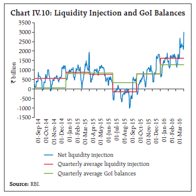 As pointed out earlier in this chapter, liquidity tightness in Q4 is a recurring phenomenon, especially in March. Among the major frictional drivers of liquidity, larger than usual swings in Government balances necessitated stepping up offsetting net LAF injection/absorption operations this year (Chart IV.10). Additional headroom was also provided within the prescribed SLR for accommodating the maintenance of higher LCR, which alleviated liquidity concerns by freeing up excess SLR to be used for collateralised money market/LAF transactions2. These operations were reflected in the growth of reserve money at 14.5 per cent*, significantly higher than the growth in nominal GDP at 8.6 per cent in 2015-16. Moreover, there was a large overhang of permanent liquidity injected in 2014-15, when net foreign currency asset purchases (adjusted for OMO sales) were as high as 190 per cent of the increase in currency. Broad money (M3) growth trailed the growth in reserve money in the second half of the year, mirroring modest deceleration in growth of deposits and the impact of relatively higher growth in currency on the money multiplier. 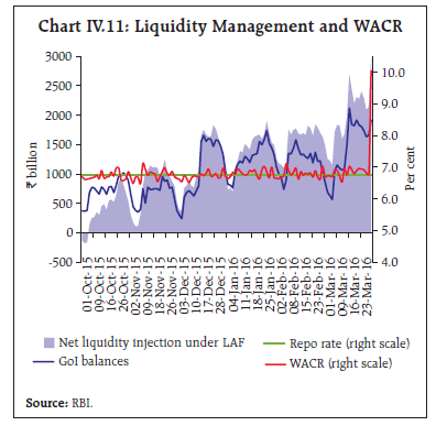 With proactive liquidity management, the effective policy corridor in the second half of the year was +36/-27 bps** pointing to the marksmanship achieved in terms of the Reserve Bank’s operating target, notwithstanding perceptions about persisting deficit liquidity (Chart IV.11). The WACR spread over the repo rate, in fact, remained within +/-10 bps on 50 per cent of the total number of trading days, and within +/- 20 bps on 85 per cent of the total number of trading days. In this context, the issue of the appropriate width of the liquidity management corridor assumes significance (Box IV.1). Box IV.1: Tactical Marksmanship in Liquidity Management Corridor systems widely adopted by central banks in their monetary policy operations encounter both consensus and dilemmas or trade-offs. There is consensus that: (a) the operating target should be an interest rate over which the central bank has the most control – the overwhelming preference in country practices is for the overnight money market rate; (b) a sound and active liquidity management framework is essential to steer the target rate close to the policy rate; (c) there is a commitment to smoothing volatility in the target rate; and (d) reasonably accurate liquidity forecasts drive the active liquidity operations. The dilemmas include: (i) which instrument to use for modulating liquidity conditions; (ii) which interest rate to target – collateralised or uncollateralised, and overnight or short-term; and (iii) width of the corridor – too wide a corridor allows volatility in the operating target while too narrow a corridor disincentivises market development. International experience suggests that a preference for narrowing the policy rate corridor has generally been driven by the emphasis on minimising volatility in the overnight rate, as too wide a corridor appears to distort policy signals (Maehle, 2014) and encourages liquidity hoarding (Gray, 2013). Trading risks associated with high volatility may, in fact, dent market development, and market feedback in a volatile market for fine tuning liquidity operations may also become noisier. Countries with narrow symmetrical corridors (+/- 25 bps in the case of Australia and Canada) seem to ‘middle’ their operating targets better since market participants are encouraged to borrow and lend among themselves rather than use the central bank’s facilities (Table 1). The Bank of Thailand established a corridor of +/-50 bps in 2006, and did not have to change it thereafter as it helped in achieving the target in both normal and crisis times. The Bank of England switched to a symmetrical +/-25 bps corridor in 2006, after experimenting with the asymmetrical +150/-100 bps corridor earlier. Volatility dropped significantly after the switchover. The Riksbank in 2000 started with a corridor of +/-75 bps but after the global crisis, the corridor was narrowed to +/-50 bps in 2009. In India, the stylised evidence shows that volatility in the operating target has reduced markedly over the years. Rolling period standard deviations of the call rate for 7 days to 90 days have declined to a tenth from 4.5 per cent in 2006-07 to around 0.4 per cent in 2014-15 and further to 0.2 per cent in 2015-16. The efficacy of the revised liquidity management framework in reducing volatility in the overnight money markets is also validated by conditional volatility estimated by an I-GARCH (1, 1) model: spikes now occur with a reduced frequency. Fleetness in anticipating and responding to market aberrations has played an important role in these recent outcomes. Even intra-period reserve maintenance flux is getting evened out and final maintenance day effects are statistically insignificant. | Table 1: Spread of Mean of Interbank Rate versus Target Rate: Select Countries1 | | (Percentage points) | | Country | During Crisis | Post Crisis | | Aug 9, 2007- Dec 2010 | Jan, 2011- Dec, 2012 | 2013 | 2014 | 2015 | | Australia | 0.00 | 0.00 | 0.00 | 0.00 | 0.00 | | Canada | 0.10 | 0.00 | 0.00 | 0.00 | 0.00 | | Sweden | -0.06 | 0.17 | 0.05 | 0.05 | 0.01 | | UK | 0.07 | 0.05 | -0.02 | -0.03 | -0.02 | | Euro Area | -0.40 | -0.50 | -0.50 | -0.10 | -0.10 | | Czech Rep | 0.07 | 0.09 | 0.13 | 0.10 | 0.10 | | Poland | -0.54 | -0.25 | -0.14 | -0.06 | -0.07 | | Hungary | -1.15 | -1.62 | -1.25 | -1.52 | -1.23 | | US | -0.13 | 0.00 | | | | | Switzerland | -1.11 | -0.51 | -0.52 | -0.51 | -1.19 | | Norway | 0.14 | 0.00 | 0.00 | -0.01 | -0.01 | | New Zealand | -0.11 | -0.07 | -0.03 | -0.04 | -0.09 | References: 1 Patra, M.D., Kapur M, Kavediya R, and Lokare S.M. (2015) “Liquidity Management and Monetary Policy: From Corridor Play to Marksmanship” in ‘Monetary Policy in India: A Modern Macroeconomic Perspective’, Springer Verlag, 2016 forthcoming. Gray, S. et al., (2013), “Monetary Issues in the Middle East and North Africa”, Departmental Paper, IMF. Maehle, N. (2014), “Monetary Policy Implementation: Operational Issues for Countries with Evolving Monetary Policy Regimes”, https://www.imf.org/external/np/seminars/eng/2014/oapbali/pdf/M3.pdf. IV.3 Global Spillovers and Domestic Financial Markets Various segments of the domestic financial market spectrum have been impacted by bouts of turmoil in global financial markets and heightened volatility. In view of the disruptions in normal functioning of these markets and the implications for monetary policy transmission, identifying, measuring and managing spillovers has become a major challenge for domestic macroeconomic policies. In India, both domestic factors and global spillovers have conditioned movements in financial markets, though increasingly domestic factors appear to have played a more prominent role. Money, bond and credit markets are largely insulated in terms of persistence of the impact on average price levels, unlike the foreign exchange and stock markets. However, global spillovers tend to influence volatility in all segments3. Among domestic factors, liquidity conditions, market microstructure, inflation and fiscal outlook, and market concerns relating to asset quality of banks and corporate balance sheets have a prominent influence on market activity. Proactive liquidity management is critical to transmission, but by itself cannot prevent disruptions arising from overwhelming global developments.
V. External Environment Global economic activity has slackened further and international trade remains subdued, while downside risks have increased. Weak demand and soft commodity prices have rekindled fears of deflation in some key AEs, prompting renewed divergence in monetary policy stances. With fragile domestic economic fundamentals, EMEs remain vulnerable to swings in market sentiments and capital outflows. Since the MPR of September 2015, the global economy has weakened, with rising downside risks prompting downward revisions to forecasts by several international agencies. Still subdued commodity prices and trade flows coupled with rising volatility in capital flows, exchange rates and financial markets have amplified the downside risks more recently. Stagnant investment across economies remains the main drag on growth. Clouding the outlook is the continuing loss of momentum in EMEs, overlaid by the anticipated slowdown in China and tightening financial conditions. Global financial markets remained relatively calm in Q4 of 2015, factoring in the US monetary policy shift to normalisation. Sentiment was boosted by monetary policy easing in China and indication of further monetary stimulus in the Euro area and Japan. In January, however, financial markets were in turmoil, with an upsurge in volatility. Fears of further weakening of the Chinese economy and the depreciation of the Renminbi (RMB) set off capital outflows from China and triggered sell-offs in equity and debt markets across AEs and EMEs. Worries about profitability of banks churned global financial markets again in February before they began recuperating in March. V.1 Global Economic Conditions The US economy slowed in the second half of 2015 as the private sector cut back capital investment in the face of an inventory glut, while a strong dollar and tepid global demand weighed on exports. Industrial production remained in contraction mode in Q1 of 2016. Consumer sentiment remained upbeat, however, despite mixed sentiment in labour market conditions and retail sales. In the Euro area, growth decelerated in Q4 of 2015 due to sagging exports, though private consumption was boosted by low oil prices and favourable financing conditions. Consumer confidence and economic sentiment have fallen significantly in Q1 of 2016. Growth in the Japanese economy suffered a setback in Q4 of 2015 as the fall in private consumption overshadowed the expansion in exports. Continuing decline in factory output amplifies the fear of contraction in GDP in Q1 of 2016. The UK economy picked up in Q4 of 2015, driven by its services sector. Business confidence, however, remains subdued in Q1 of 2016 (Table V.1). | Table V.1: Real GDP Growth (q-o-q, annualised) | | (Per cent) | | Period | Q1-2015 | Q2-2015 | Q3-2015 | Q4-2015 | 2016 (P) | | Advanced Economies | | US | 0.6 | 3.9 | 2.0 | 1.4 | 2.6 | | Euro area | 2.0 | 1.6 | 1.2 | 1.2 | 1.7 | | Japan | 4.6 | -1.4 | 1.4 | -1.1 | 1.0 | | UK | 1.6 | 2.4 | 1.6 | 2.4 | 2.2 | | Canada | -0.8 | -0.4 | 2.4 | 0.8 | 1.7 | | Korea | 3.2 | 1.6 | 5.2 | 2.8 | 3.2 | | Emerging Market and Developing Economies | | China | 5.2 | 7.6 | 7.2 | 6.4 | 6.3 | | Brazil | -3.3 | -8.2 | -6.8 | -5.8 | -3.5 | | Russia | -4.6 | -5.2 | -2.3 | | -1.0 | | South Africa | 1.4 | -1.3 | 0.7 | 0.6 | 0.7 | | Thailand | 2.0 | 1.6 | 4.0 | 3.2 | 3.2 | | Malaysia | 4.8 | 4.4 | 2.8 | 6.0 | 4.5 | | Mexico | 2.1 | 2.6 | 3.3 | 2.2 | 2.6 | | Saudi Arabia* | -2.4 | 0.3 | 1.8 | | 1.2 | | Memo Items: | 2013 | 2014 | 2015 E | 2016 P | 2017 P | | World Output | 3.3 | 3.4 | 3.1 | 3.4 | 3.6 | | Advanced Economies | 1.1 | 1.8 | 1.9 | 2.1 | 2.1 | | Emerging Market and Developing Economies | 5.0 | 4.6 | 4.0 | 4.3 | 4.7 | | World Trade Volume | 3.3 | 3.4 | 2.6 | 3.4 | 4.1 | | E: Estimate P: Projection *: Seasonally unadjusted Sources: Bloomberg and IMF. | In EMEs, the overall macroeconomic environment remains challenging, with growth having weakened further in recent quarters. Their relative contribution to world output growth shrank in 2015 (Chart V.1). The Chinese economy recorded the lowest quarterly expansion in Q4 of 2015 since 2009, with downside risks looming large in terms of weak external demand, factory overcapacity, slowing investment, a soft property market and high debt levels. Recessionary conditions persisted in Brazil in the closing quarter of 2015, as worsening labour market conditions and falling fuel and electricity subsidies continue to adversely impact private consumption. Investment was hamstrung by a combination of low domestic demand, high borrowing costs and weak business confidence. In Russia, economic activity remained in contraction. South Africa continued to face severe droughts, coupled with a plunging currency and political turmoil. By contrast, Turkey, Indonesia, Thailand and the Philippines recorded improved growth. Going forward, the OECD’s latest composite leading indicators suggest tentative signs of stabilisation in China and a loss of momentum in Brazil and Russia (Chart V.2). 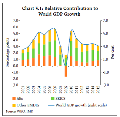 Global cross-border trade flows remained weak in 2015 and in January 2016 as well, propagated largely through manufacturing and investment linkages. Reduced demand for imports from China, sluggish importintensive investment in other EMEs, particularly in extractive industries, and increasingly unremunerative terms of trade have played important roles. Nevertheless, trade volume has shown some resilience (Chart V.3). Looking ahead, a modest improvement in world trade flows is projected by the International Monetary Fund (IMF) and World Bank in 2016. V.2 Commodity Prices and Global Inflation Global commodity prices softened further through Q4 of 2015. A recent uptick starting in mid-February 2016 is shadowed by excess supply, faltering demand from EMEs and strengthening of the US dollar. Crude oil prices dipped to a 12-year low of below US$ 30 per barrel in January 2016 under the weight of supply glut, combined with weaker than expected demand due to a milder winter in the northern hemisphere. The weakening US dollar and anticipation of OPEC freezing output in its scheduled April meeting, however, has boosted crude oil prices lately. Metal prices fell for four consecutive months till January; however, prices of gold gained by around 16 per cent during Q1of 2016 as demand for safe haven assets increased. Agricultural prices, which declined in Q4 of 2015, rose marginally for two consecutive months up to February due to supply concerns arising from still intense El Nino conditions (Chart V.4a and b). 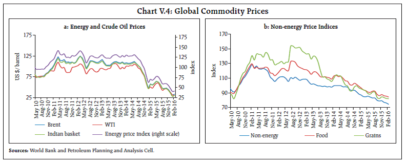 Globally, inflation pressures were contained by weak global growth and the continuing softness in commodity prices. In the US, inflation inched up since the beginning of Q4 of 2015 through January, but it eased in February and is expected to remain well below 2.0 per cent in the near- term. The Euro area slipped back into deflation in February, after experiencing a creeping up of inflation in the three months up to January. Similarly, in Japan, inflation remains near zero since Q4 of 2015, and downside risks persist. By contrast, a number of EMEs continue to reel under high inflation due to currency depreciation – in Brazil, Russia and other Latin American countries – and domestic structural rigidities - in South Africa and Turkey (Chart V.5a and b). Thailand and Korea have benefited from low commodity prices, and inflation has eased below target since late 2012 and early 2013, respectively. V.3 Monetary Policy Stance Monetary policy stances have been diverging across both AEs and EMEs. In December 2015, the Fed raised its policy rate after almost a decade – to a target range for the fed funds rate of 0.25-0.5 per cent. However, the future policy rate path of Fed remains uncertain with the rate being kept on hold in January and March alongside dovish guidance. On the other hand, as fears of growth slowdown and deflation resurfaced, Japan and the Euro area have further eased unconventional accommodation. The European Central Bank (ECB) expanded its QE programme in March, reduced the deposit rate further into negative territory (-0.4 per cent) and cut its policy rate to zero. The Bank of Japan (BoJ), while maintaining its quantitative and qualitative easing programme, introduced a negative deposit rate since January. While the aim of countries pursuing negative interest rates has been to improve domestic growth and inflation outlook, it has given rise to global concerns about financial stability (Box V.1). Box V.1: Negative Interest Rate-Crossing the Last Frontier Post the Great Financial Crisis, Sveriges Riksbank, Danmarks Nationalbank, the ECB, the Swiss National Bank and, most recently, the BoJ have introduced negative interest rates on deposits at the central bank, and lowered the target for the overnight rate to below zero in some of them. Although the overall objective has been to raise economic growth and counter deflationary conditions by deterring saving, and encouraging borrowing and risk taking, scepticism has developed about the efficacy of the policy in achieving anything beyond inflating asset prices and depreciating currencies competitively. First, banks may choose to borrow less from the central bank in order to lower excess reserves and avoid the negative deposit rate. This would put upward pressure on rates in the interbank and bond market, offsetting the stimulative impact of the negative policy rate. Second, even if negative interest rates are transmitted to money markets, retail deposits may remain insulated due to banks’ reluctance to pass it on to depositors for fear of losing deposits. Third, there could be offsetting adjustment in lending rates among sectors such as in Switzerland where negative rates have led to a rise in mortgage rates to protect margins. Fourth, unless there is transmission of the negative interest rate into lending and deposit rate, it would lose its rationale of boosting domestic demand. Lastly, if persisted for long, negative interest rates may encourage financial excesses, including instruments that emulate currency, allow tax avoidance and undermine the policy itself. As for actual outcomes, negative interest rates could be impacting profit margins of banks already - concerns about profitability of banks in early February 2016 led to a sharp fall in bank equities in the Euro area which spread across AEs and EMEs. Over time, this could get entangled with volatility in financial markets due to persistent mispricing and financial imbalances, setting them up for the shocks from inevitable corrections. It is also observed that under negative interest rates, a tendency for resorting to currency depreciation to attract foreign demand gets heightened (Lipton, 2016). A simple event-study analysis corresponding to day/ month/quarter of introduction of the policy shows uncertain impacts on both GDP and inflation as well as perverse outcomes - decline in GDP growth and deeper deflation in Switzerland (Chart a and b). However, the counterfactual remains that the situation could have been worse without the policy. References: Hannoun, Herve (2015), “Ultra-low or Negative Interest Rates: What They Mean for Financial Stability and Growth”, Remarks at the Eurofi High-Level Seminar, Riga, April 22. Lipton David (2016), “Policy Imperatives for Boosting Global growth and Prosperity”, Speech delivered at National Association for Business Economics, Washington, D.C. Monetary policy in EMEs has also been diversely stanced, reflective of varied macroeconomic conditions. China has aggressively cut deposit and lending rates and relaxed required reserves, including in March, to modulate the pace of economic slowdown. Indonesia, which lowered reserve requirements to boost bank financing capacity in November, reduced the policy rate in January and February on growth concerns. By contrast, South Africa raised its policy rate in November 2015 and January 2016 to curb inflationary pressures. Brazil and Russia continue to maintain high policy rates despite recession, as inflationary pressures remain elevated by large currency depreciation. Some Latin American countries such as Mexico, Chile and Colombia have been raising policy rates in response to currency depreciation, tracking in some measure the depreciation of the RMB (Chart V.6a and b). V.4 Global Financial Markets Global financial markets began Q4 of 2015 on a positive note, with market sentiment boosted by the Fed refraining from raising policy rate in its September meeting. As concerns about China seemed to recede, markets rallied in October – globally, equity markets recorded modest gains, yields softened in debt markets, major currencies regained some ground against the US dollar and crude oil traded briefly above US$ 50 per barrel for the first time since July. Policy interventions in major EMEs and AEs, either through stepping up of monetary accommodation or intervention in foreign currency markets, also supported the markets. With a hawkish tone discernible in Fed’s October meeting, both money and bond markets in the US reacted to heightened rate expectations that gained ground from November 2015. In the Euro area, however, market sentiment remained calm until December. 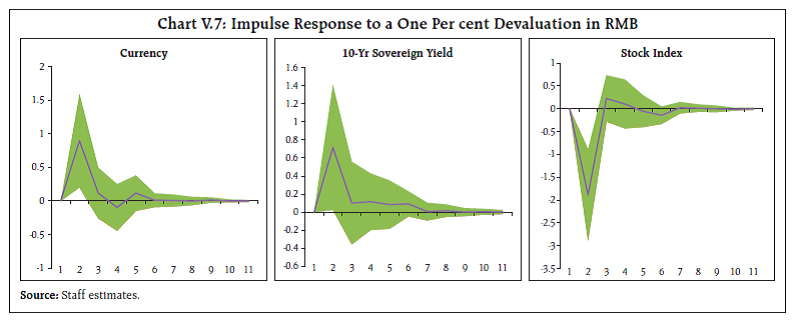 Since the beginning of 2016, fears about weakening global growth have re-emerged, especially about China. Combined with worries about financial viability of European banks and falling commodity prices, it triggered surges of volatility in financial markets and overshoots, with contagion spreading to financial markets across AEs and EMEs. A panel VAR using daily data of select EMEs for the period July 1, 2015 to February 25, 2016 - covering the two episodes of large devaluation in RMB in August 2015 and January 2016 - shows that devaluation of the RMB induces marked movement in the currency, bond and equity markets in the panel countries over the next two weeks.1 A one per cent depreciation in the RMB leads to a similar depreciation in the currencies of these countries, while the 10-year G-sec yield hardens and equity prices fall significantly (Chart V.7). 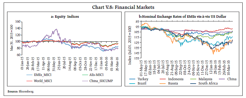 Global equity markets dipped into ‘bear’ territory during January-February 2016, with equity prices retreating across all major markets. Bank equities, in particular, were hit hard in AEs and have fallen significantly since the beginning of the year - 21 per cent in the Euro area; 30 per cent in Japan; 19 per cent in the UK; and 12 per cent in the US. Equity markets also fell across EMEs in Q1 of 2016, but the declines were relatively modest (Chart V.8a). In AE bond markets, yields rose in the last quarter of 2015 on the anticipated rate hike by the Fed and easing concerns about China. Net foreign portfolio flows to EME bond markets were mostly negative in Q4 which kept yield rates high. In Q1 of 2016, financial market turbulence and a further sharp fall in oil prices aggravated worries about global growth, and government bond yields fell into negative territory in some AEs. The introduction of a negative deposit rate by Japan pushed its 10-year bond yield into negative zone, which spurred demand for other positive yielding treasuries and depressed their yields. Global foreign exchange markets broadly tracked the equity markets, policy measures of central banks in systemically important economies and shifts in investors’ risk assessments. The US dollar has generally strengthened, barring intermittent loss of ground on incoming data. Currency markets have reacted perversely to more recent unconventional monetary policy actions by the ECB and the BoJ, with appreciation in the euro and yen occurring immediately after policy announcements. Among EME currencies, a few currencies such as the Korean won, the Malaysian ringgit, the Thai Baht and the Indonesian rupiah appreciated in Q4 of 2015. By contrast, currencies such as the Brazilian real, the Russian ruble and the South African rand weakened due to lower commodity prices. Most EME currencies have steadied after losing ground in early part of Q1 of 2016 (Chart V.8b). In sum, downside risks to global economic activity have increased. With global commodity prices and inflation expected to remain soft, monetary policy stances continue to be highly accommodative, but divergent. Financial markets remain vulnerable to volatility and flux in capital flows and investor sentiment.
ABBREVIATIONS | AE | Advance Estimates | | AEs | Advanced Economies | | AQR | Asset Quality Review | | BE | Budget Estimates | | BoJ | Bank of Japan | | bps | Basis Points | | BRICS | Brazil, Russia, India, China and South Africa | | CBLO | Collateralised Borrowing and Lending Obligation | | CDs | Certificates of Deposit | | CI | Confidence Interval | | CII | Confederation of Indian Industry | | CMIE | Centre for Monitoring Indian Economy | | CPs | Commercial Papers | | CPC | Central Pay Commission | | CPI | Consumer Price Index | | CPI-AL | Consumer Price Index-Agricultural Labourers | | CPI-IW | Consumer Price Index-Industrial Workers | | CPI-RL | Consumer Price Index-Rural Labourers | | CSO | Central Statistics Office | | CU | Capacity Utilisation | | DA | Dearness Allowance | | DISCOMs | Distribution Companies | | ECB | European Central Bank | | EMDEs | Emerging Markets and Developing Economies | | EMEs | Emerging Market Economies | | FDI | Foreign Direct Investment | | FICCI | Federation of Indian Chambers of Commerce and Industry | | FIT | Flexible Inflation Targeting | | FMCG | Fast-moving Consumer Goods | | FOMC | Federal Open Market Committee | | FPIs | Foreign Portfolio Investors | | FY | Financial Year | | GARCH | Generalised Autoregressive Conditional Heteroskedasticity | | GDP | Gross Domestic Product | | GFD | Gross Fiscal Deficit | | GNDI | Gross National Disposable Income | | G-Secs | Government Securities | | GVA | Gross Value Added | | H1 | First Half of the Year | | H2 | Second Half of the Year | | HQLA | High Quality Liquid Asset | | HRA | House Rent Allowance | | IIP | Index of Industrial Production | | IMD | India Meteorological Department | | IMF | International Monetary Fund | | INR | Indian Rupee | | IPO | Initial Public Offering | | LAF | Liquidity Adjustment Facility | | LCR | Liquidity Coverage Ratio | | LIBOR | London Interbank Offered Rate | | LHS | Left Hand Side | | LPA | Long-period Average | | LPG | Liquefied Petroleum Gas | | M3 | Money Supply | | MCLR | Marginal Cost of Funds Based Lending Rate | | m-o-m | Month-on-Month | | MPC | Monetary Policy Committee | | MPFA | Monetary Policy Framework Agreement | | MPR | Monetary Policy Report | | MSP | Minimum Support Price | | NCAER | National Council of Applied Economic Research | | NCR | National Capital Region | | NDTL | Net Demand and Time Liabilities | | NEER | Nominal Effective Exchange Rate | | NPA | Non-performing Asset | | OIS | Overnight Indexed Swap Rate | | OMOs | Open Market Operations | | OPEC | Organisation of Petroleum Exporting Countries | | OROP | One Rank One Pension | | PFCE | Private Final Consumption Expenditure | | PMI | Purchasing Managers’ Index | | POL | Petroleum, Oil and Lubricant | | PSU | Public Sector Unit | | Q | Quarterly | | q-o-q | Quarter-on-Quarter | | RBI | Reserve Bank of India | | RE | Revised Estimates | | REER | Real Effective Exchange Rate | | RHS | Right Hand Side | | RMB | Renminbi | | RRBs | Regional Rural Banks | | ₹ | Indian Rupee | | SAAR | Seasonally Adjusted Annualised Rate | | SLR | Statutory Liquidity Ratio | | T-Bill | Treasury Bill | | UDAY | Ujwal DISCOM Assurance Yojana | | UK | United Kingdom | | US | United States | | UVI | Unit Value Index | | VAR | Vector Autoregression | | WACR | Weighted Average Call Money Rate | | WALR | Weighted Average Lending Rate | | WADTDR | Weighted Average Domestic Term Deposit Rate | | WAR | Weighted Average Rate | | WEO | World Economic Outlook | | WPI | Wholesale Price Index | | y-o-y | Year-on-Year | |