“The Bank shall publish a document explaining the steps to be taken by it to implement the decisions of the Monetary Policy Committee, including any changes thereto” [Section 45ZJ(1) of the Reserve Bank of India Act, 1934] 1. Introduction IV.1 The operating procedure of monetary policy1 revolves around the implementation of monetary policy decisions – “the plumbing in its architecture” (Patra et al., 2016). As enjoined by the RBI Act, the decision of the MPC on the policy rate has to be operationalised by the RBI so that it alters the spending behaviour of economic agents and, in turn, achieves the RBI’s mandate on inflation and growth. Since monetary policy is characterised by “inside” and “outside” lags in policy formulationand implementation,2 the challenge for an efficient operating procedure is to (i) minimise the transmission lag from changes in the policy rate to the operating target – a variable that can be controlled by monetary policy actions – rapidly and efficiently; and (ii) ensure that changes in the operating target are transmitted as fully as feasible across the interest rate term structure in the economy. In pursuit of the legislative mandate, details of the changes in operating procedure and their rationale are presented in the bi-annual Monetary Policy Reports. IV.2 The weighted average call rate (WACR) – which represents the unsecured segment of the overnight money market and is best reflective of systemic liquidity mismatches at the margin – was explicitly chosen as the operating target of monetary policy in India. An interest rate corridor – the liquidity adjustment facility (LAF) – has been defined since May 2011 by the interest rate on the marginal standing facility (MSF) as the upper bound (ceiling), the fixed overnight reverse repo rate as the lower bound (floor) and the policy reporate in between (RBI, 2011).3 IV.3 The LAF corridor effectively defines the operating procedure of monetary policy. Once the policy repo rate is announced, liquidity operations are conducted to keep the WACR closely aligned to the repo rate. While the operating target and the LAF corridor framework have remained unchanged during the FIT period, several refinements have been introduced regarding (i) the width of the corridor; (ii) the choice of liquidity management instruments; and (iii) finetuning regular/durable market operations, all intended to anchor the term structure of interest rates to the policy repo rate in order to strengthen transmission. IV.4 Monetary policy transmission constitutes a ‘black box’ (Bernanke and Gertler, 1995). Several channels of transmission have been identified in the literature and the cross-country experience: (i) the interest rate channel described in the foregoing; (ii) the credit or bank lending channel, which assumes importance in a bank-dominated financial system such as India’s; (iii) the exchange rate channel operating through relative prices of tradables and non-tradables; (iv) the asset price channel impacting wealth/income accruing from holdings of financial assets; and (v) the expectations channel encapsulating the perceptions of households and businesses on the state of the economy and its outlook. These conduits of transmission intertwine and operate in conjunction and are difficult to disentangle. There is a loose consensus, however, in great measure associated with the development and growing sophistication of financial markets, that the interest rate channel is dominant (Bernanke and Blinder, 1992). Since the 2000s, this has provided the rationale for the choice of the operating procedure in India. During FIT, this operating procedure has been reinforced by practitioner innovations and communication strategies. In the process, trade-offs have surfaced, which warrant careful evaluation in order to draw lessons for the operationalisation of FIT in India, going forward. IV.5 Given this motivation, this chapter sets out to review the performance of the extant operating framework and its efficacy. The rest of the Chapter is structured in the following manner: Section 2 presents the stylised facts of the operating procedure and the transmission mechanism juxtaposed against the cross-country experience. Section 3 addresses specific tensions stemming from the operating procedure and the monetary transmission mechanism, some aspects of which engaged public discourse over the past four years. This section also recommends steps needed to fine-tune the operating procedure and facilitate better transmission. Finally, Section 4 concludes by laying out the challenges lying ahead. 2. Some Stylised Facts IV.6 Refinements in the operating framework have been undertaken in response to the changing macroeconomic and financial environment to sharpen the role of the repo rate as the single policy rate, to establish the 14-day term repo as the main instrument for providing liquidity over the reserve maintenance period and to enable a flexible framework that could shift seamlessly from a deficit mode in consonance with a tightening stance to a surplus mode in support of an accommodative stance (Table IV.1). IV.7 In February 2020, the culmination of these reforms was placed in the public domain with a view to clearly communicating the objectives and the toolkit for liquidity management (Box IV.1). IV.8 During the period of FIT,4 liquidity management operations underwent severe stress on two occasions. The first test came with the surplus liquidity glut post-demonetisation, which prompted the RBI to impose an unprecedented incremental cash reserve ratio (CRR) of 100 per cent for one fortnight (RBI, 2017). The second shock is the outbreak of COVID-19 when market seizure caused a collapse in trading activity, warranting the use of extraordinary system-wide as well as targeted liquidity measures to restore normalcy (RBI, 2020). | Table IV.1: Reforms in the Operating Framework | | The New Operating Framework of Monetary Policy (May 2011) | Revised Liquidity Management Framework (September 2014) | Modified Liquidity Framework (April 2016) | • Repo Rate - Single policy rate. • Weighted average overnight call money rate (WACR) is the operating target. • Corridor of +/- 100 bps around the Repo Rate. • 100 bps above the repo rate for the Marginal Standing Facility (MSF) and 100 bps below the repo rate for the reverse repo rate. • Full accommodation of liquidity demand at the fixed repo rate, albeit with an indicative comfort zone of +/-1 per cent of net demand and time liabilities (NDTL) of the banking system. • Transmission of the changes in Repo Rate through the WACR to the term structure of interest rates. | • Access to assured liquidity of about 1 per cent of NDTL on an average • Bank-wise overnight fixed rate repos of 0.25 per cent of NDTL, and the balance through 14-day variable rate term repos. • More frequent auctions of 14-day term repos during a fortnight (every Tuesday and Friday of a week). • Introduction of variable rate fine-tuning repo/reverse repo auctions. | • The corridor around the Repo rate narrowed from +/- 100 bps to +/- 50 bps. • Commitment to progressively lower the ex-ante system level liquidity deficit to a position closer to neutrality in the medium run. • Reducing the minimum daily maintenance of the CRR from 95 per cent of the requirement to 90 per cent. |
Box IV.1
Liquidity Management Framework The salient features of the extant framework operationalised on February 14, 2020 are5: The liquidity management corridor is retained and the weighted average call rate (WACR) remains the operating target. The width of the corridor was retained at 50 basis points (bps)6 A 14-day term repo/reverse repo operation at a variable rate and conducted to coincide with the cash reserve ratio (CRR) maintenance cycle is the main liquidity management tool for managing frictional liquidity requirements; the daily fixed rate repo and four 14- day term repos conducted every fortnight earlier stand withdrawn. The main liquidity operation is supported by fine-tuning operations, overnight and/or longer tenor, to tide over any unanticipated liquidity changes during the reserve maintenance period; if required, the RBI will conduct variable rate repo/reverse repo operations of more than 14 days tenor. Liquidity management instruments include fixed and variable rate repo/reverse repo auctions, outright open market operations (OMOs), forex swaps and other instruments. The daily minimum CRR maintenance requirement is retained at 90 per cent7 Standalone Primary Dealers (SPDs) are allowed to participate directly in all overnight liquidity management operations. Transparency in communication is enhanced through (a) dissemination of both flow and stock impact of liquidity operations; and (b) publication of a quantitative assessment of durable liquidity conditions of the banking system with a fortnightly lag. | Operating Framework and Market Microstructure IV.9 The choice of the operating framework and the liquidity management strategy of a central bank is premised on an efficient inter-bank money market which ensures smooth transfer of funds from lenders to borrowers and, in that process, determines the overnight rate (Bindseil, 2014). Reforms to develop the money market in India over the years in the context of the first leg of monetary policy transmission have expanded participation and instruments. There has been a steady migration of market activity to collateralised segments (Table IV.2), in conformity with some advanced economy (AE) experiences viz., the US, the UK, the Euro area and Japan. IV.10 In the uncollateralised segment, the reduced turnover is highly concentrated in the opening and the closing hours of trading, which tends to accentuate volatility in the WACR (Bhattacharyya et al., 2019). The collateralised segments are dominated by non-bank participants such as mutual funds (MFs). Consequently, extraneous developments such as large redemption pressures in the stock market spill over and bring episodes of tightness to overnight market conditions. Likewise, regulatory changes that mandate or incentivise collateralised instruments for investment by these entities – as in September20198 – can ease market conditions unexpectedly. Other aspects of the market microstructure can also influence the WACR. Specifically, special repos – repo transactions in which funds are lent in order to acquire a specific security for meetingobligations in the short sale9 market – often drive market repo rates to unduly low levels, dragging down money market rates out of sync with the Reserve Bank’s operating corridor. Furthermore, a higher proportion of ‘reported deals’ – which are traded over-the-counter (OTC) and reported on the negotiated dealing system (NDS)-Call platform after the deals are completed – exerts adisproportionate influence on the WACR.10 | Table IV.2: Share in Overnight Money Market Volume | | (Per cent) | | Financial Year | Uncollateralised | Collateralised | | Call Money | CBLO/ Tri-party Repo | Market Repo | | Pre-FIT | 2011-12 | 21.2 | 58.9 | 19.9 | | 2012-13 | 21.1 | 54.5 | 24.5 | | 2013-14 | 15.2 | 60.1 | 24.8 | | 2014-15 | 13.0 | 59.2 | 27.8 | | 2015-16 | 12.4 | 59.1 | 28.6 | | 2016-17 (April - September) | 11.5 | 56.2 | 32.3 | | Average (Pre-FIT) | 15.4 | 58.2 | 26.4 | | FIT | 2016-17 (October – March) | 9.8 | 61.4 | 28.8 | | 2017-18 | 8.4 | 63.2 | 28.5 | | 2018-19 | 9.6 | 63.8 | 26.6 | | 2019-20 | 6.9 | 68.0 | 25.1 | | Average (FIT) | 8.4 | 64.8 | 26.8 | Note: Tri-party repo replaced collateralized borrowing and lending obligations (CBLO) effective November 5, 2018; Pre-FIT (April 2011- September 2016).
Source: Reserve Bank of India (RBI). | Policy Corridor IV.11 During FIT, liquidity management operations kept the WACR within the policy corridor on 97 per cent of the time (Table IV.3), although it predominantly traded below the repo rate (91 per cent of the time). IV.12 The country experience with regard to a corridor system indicates that the operating target generally lies in the middle, i.e., equidistant from the ceiling and the floor, suggesting efficient liquidity management based on prescient forecasting of systemic liquidity requirements (Sveriges Riksbank, 2014). In India, the WACR was centred in the LAF corridor and aligned tightly with the policy rate ahead of the institution of FIT and through its early months, reflecting monetary marksmanship on the back of a narrowing of the corridor from 200 bps in April 2015 to 50 bps by April 2017. This was honed by active liquidity management – 14-day repo auctions were used in the place of fixed rate repo. From the latter part of 2016-17 and in the first half of 2017-18, the demonetisation-induced liquidity overhang imparted a softening bias to overnight rates, reflected in a negative spread (over the repo rate) of 19 bps over a year. In the wake of the slowdown in economic activity thereafter, the RBI adopted an accommodative stance of monetary policy and allowed systemic liquidity (net LAF) to transit from deficit to surplus from June 2019 and into large liquidity absorption with the onset of the pandemic (Chart IV.1a). Overall, the WACR traded 11 bps below the repo rate under FIT on average, as against 19 bps above the repo rate pre-FIT (Chart IV.1b). 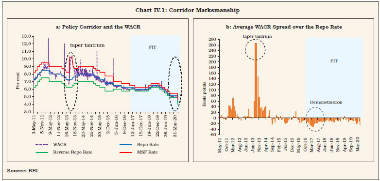
| Table IV.3: Operating Target and Monetary Marksmanship | | (Days) | | Regime | Outside Corridor | Within Corridor | Total | | > MSF | < Reverse Repo | < Repo | = Repo | > Repo | | Pre-FIT | 31 | 0 | 556 | 7 | 710 | 1,304 | | FIT | 4 | 23 | 742 | 2 | 74 | 845 | | Overall | 35 | 23 | 1,298 | 9 | 784 | 2,149 | Note: Pre-FIT: (May 2011 to September 2016); FIT: (October 2016 to March 2020).
Source: RBI. | IV.13 The country experience suggests that the corridor width usually ranges between 25-200 bps around the policy rate/target (Annex IV.1). The optimal width of the corridor and its impact on liquidity management has been extensively deliberated in the literature. A wider corridor is synonymous with costlier central bank standing facilities and is associated with (i) greater inter-bank turnover; (ii) leaner balance sheet of the central bank; and (iii) greater short-term interest rate volatility (Bindseil and Jablecki, 2011). In contrast, a narrow corridor is associated with (i) shrinking inter-bank market activity; (ii) higher recourse to standing facilities, leading to a sharp increase in the size of the central bank’s balance sheet; and (iii) stable short-term rates in the inter-bank market. In India, the width of the corridor was progressively narrowed in a symmetric manner, which helped in moderating volatility – measured by the exponential weighted moving average(EWMA)11 of the WACR – corroborating the cross-country experience (Chart IV.2). IV.14 An asymmetric corridor has also been proposed in the context of a weak economy and a fragile financial sector (Goodhart, 2010); in practice, it has gained wide acceptability among some AEs after the GFC. In India too, the RBI asymmetrically widened the corridor to 400 bps in mid-July 2013 in response to the taper tantrum. With the return of normalcy, the corridor width was gradually restored to its pre-crisis level of 200 bps by end-October 2013 (Chart IV.3). After the COVID-19 pandemic, the Reserve Bank once again asymmetrically widened the corridor during March-April 2020, operating a de facto floor system as various conventional and unconventional measures flooded liquidity into the system and kept financial conditions ultra-easy to counter the pandemic. Reserve Maintenance and Averaging IV.15 Although the efficacy of the CRR as a policy instrument is limited in a modern financial system, it is a potent tool for stabilising overnight interest rates by creating the demand for reserves. Banks may frontload (backload) their maintenance at the beginning (end) of the reserve maintenance period, depending on the prevailing market interest rate and expectations of future rates. Accordingly, the overwhelming preference across jurisdictions is to stipulate reserve maintenance on an average basis: maintenance periods vary from two weeks (India) to six-eight weeks coinciding with monetary policy meetings (Euro area). The number of central banks stipulating daily minimum reserve maintenance is limited (Annex IV.1). 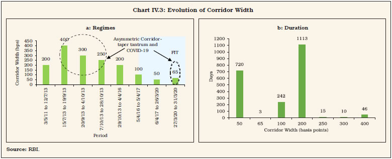 IV.16 Under Section 42(2) of the RBI Act, 1934, banks are required to maintain a specified proportion of their net demand and time liabilities (NDTL) as CRR balances with the RBI on an average daily basis over a reporting fortnight, with a minimum daily maintenance (stipulated as a proportion of actual requirements) during the fortnight. The daily minimum reserve requirement provides banks with flexibility in optimising their reserve holdings, depending upon intra-fortnight cash flows. Within the reporting fortnight, banks choose their daily maintenance levels – based on a cost-benefit analysis of interest rate expectations vis-à-vis the rates on standing facilities. Significant improvement in liquidity planning and reserve maintenance by banks has been observed in the FIT period (Chart IV.4a). The daily minimum reserve requirement was enhanced from 70 per cent of required CRR (effective since December 2002) to 99 per cent in July 2013 but subsequently reduced to 95 per cent in September 2013 and further to 90 per cent in April 2016. Post the outbreak of COVID-19, the minimum requirement was further reduced to 80 per cent in March 2020. The intra-fortnight variation (across weeks) in reserve maintenance was negligible when the daily minimum was prescribed at 99 per cent after the taper tantrum; in contrast, there has been significant frontloading in the first vis-à-vis the second week when the daily minimum balance was set at 70 per cent (Chart IV.4b). 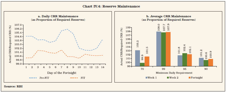 Volatility of WACR IV.17 The efficacy of monetary policy transmission is contingent upon minimising volatility in the operating target so that policy signals are not blurred. Lower volatility in the overnight inter-bank rate lessens uncertainty about funding costs (Kavediya and Pattanaik, 2016). In fact, longer term rates can be higher than the policy preference due to increased volatility in the operating target (Carpenter et al., 2016); hence, stable and predictable short-term rates can help to improve transmission (Mæhle, 2020). Minimising operating target volatility has accordingly acquired priority in liquidity management objectives of central banks. It is in this context that most central banks resort to fine-tuning operations and provide forward guidance to align the operating target with the policy rate (USA; Euro area; UK, Sweden, Canada, Norway, Australia). Volatility is also minimised by (i) synchronising main refinancing operations with the reserve maintenance periods (ECB); (ii) indexing the overnight rate to the policy rate (UK); and (iii) undertaking discretionary operations alongside regular operations. IV.18 In India, the conditional volatility of the WACR has been found to positively affect the bid-ask spread in the overnight inter-bank market (Ghosh and Bhattacharyya, 2009). The conditional volatility of WACR has generally been subdued especially after the introduction of FIT, but for the usual year-end effects associated with balance sheet adjustment by banks (Chart IV.5). IV.19 An assessment of the key determinants of volatility suggests that calendar effects (annual closing) and reserve maintenance behaviour have had lesser impact under FIT than before, indicating improved liquidity management during this period (Box IV.2). Instruments and Collateral IV.20 In the aftermath of the GFC, discretionary and emergency liquidity facilities have been active across central banks or relevant legislations are in place for their future usage, if required. Besides open market operations (OMOs), other discretionary operations include forex swaps (Australia); term deposits (Australia); compulsory deposits (Mexico); additional loans and deposits (Sweden); and funding for lending (UK). Box IV.2
Volatility of WACR – Key Determinants Based on daily data from January 2009 to March 2020, the estimated volatility of daily changes in WACR, on an average, is found to be lower during the FIT period (Table 1). Moreover, skewness and kurtosis of estimated volatility has also declined during the FIT period, which is partly reflected in the moderation of spikes in WACR around end-March during this period. High frequency variables such as the WACR exhibit volatility clustering – bouts of intense volatility followed by periods of calm. This warrants the use of generalised autoregressive conditional heteroscedasticity (GARCH) [1,1] models or variants, where the sum of the estimated parameters is close to unity. Considering the persistence of volatility in the WACR, the integrated-GARCH (I-GRACH) model is used to model volatility (Engle and Bollerslev, 1986) with the following specification:
| Table 1: Estimated Conditional Volatility of Daily Changes in WACR | | Summary Statistics | Pre-FIT$ | FIT@ | | Mean | 0.050 | 0.003 | | Median | 0.012 | 0.003 | | Maximum | 2.028 | 0.004 | | Minimum | 0.000 | 0.002 | | Std. Dev. | 0.146 | 0.000 | | Skewness | 7.308 | 0.676 | | Kurtosis | 69.882 | 2.669 | $: January 2009 to September 2016;
@: October 2016 to March 2020 |
| Table 2: Volatility of WACR | | Dependent Variable: ∆WACR | | Variables | Pre-FIT | FIT | | Mean Equation | | Constant | -0.01*** | -0.02*** | | ∑∆WACR | -0.12*** | -0.13*** | | ∑∆Repo Rate | 0.78*** | 0.49*** | | Net Liquidity | -0.00** | -0.01*** | | ECM | -0.04*** | -0.22*** | | dum_March | 3.12*** | 0.04 | | Dum_April | -3.08*** | -0.60*** | | Dum_Taper | 0.11*** | | | D3 | 0.05*** | | | D4 | 0.01*** | | | D5 | 0.01*** | | | D6 | 0.00** | | | D7 | 0.01*** | | | D10 | 0.01*** | | | D12 | 0.01*** | | | Volatility Equation | | RESID(-1)^2 | 0.23*** | 0.00* | | GARCH(-1)^2 | 0.77*** | 0.99*** | | DUM_MARCH | 0.21*** | 0.00 | | Diagnostics (p-values) | | T-DIST. DOF | 0.00 | 0.00 | | Q(10) | 0.57 | 0.31 | | Q(20) | 0.51 | 0.69 | | ARCH LM (5) | 0.86 | 0.16 | | Note: *, ** and *** denote significance at 10%, 5% and 1% level, respectively. Demonetisation dummy turned out to be insignificant in both mean and variance equation for FIT period. | A one percentage point increase in the policy repo rate led to an instantaneous increase of 0.8 percentage points in WACR in the pre-FIT period as compared with 0.5 percentage points during FIT. The error correction term, indicating the speed of adjustment for any departure of the WACR from its long-term relationship with the policy repo rate, is about five times higher for the FIT period, reflecting improvement in transmission. Calendar effects are statistically significant during both the periods; however, their impact is much lower during FIT, with the end-March effect turning insignificant. Dummy variables capturing the impact of reserve maintenance behaviour of banks turned out to be statistically significant in the pre-FIT period; however, their impact became insignificant during FIT. Reference: Engle, R.F. and T. Bollerslev, (1986), “Modelling the Persistence of Conditional Variance”, Econometric Reviews, 5, 1-50. | IV.21 For liquidity management purposes, OMOs – more purchases than sales – have been the favoured instrument in India under FIT (TableIV.4).12 USD/INR swaps have also been used since March 2019 to inject/withdraw durable liquidity. In the wake of the pandemic, unconventional monetary policy (UMP) instruments such as long-term repo operations (LTRO) and targeted long-term repo operations (TLTRO) were introduced to reach out to specific sectors, institutions and instruments, which helped in easing market stress and softening financing conditions (RBI, 2020). As a COVID-related exceptional response, refinance / line of credit was provided to All IndiaFinancial Institutions13 [viz., National Bank for Agriculture and Rural Development (NABARD); Small Industries Development Bank of India (SIDBI); National Housing Bank (NHB); and Exim Bank of India] to alleviate sector-specific liquidityconstraints.14 IV.22 Fine-tuning operations through variable rate auctions of varying maturities geared at meeting unanticipated liquidity shocks commenced from 2014-15. During FIT, these operations have increased, both in terms of volume and number of operations conducted (Table IV.5). Although the bulk of such transactions were concentrated in smaller maturities (1-3 days), reverse repo transactions of longer maturity picked up during FIT relative to before, due to phases of prolonged surplus liquidity. As a pre-emptive measure to tide over frictional liquidity requirements caused by dislocations due to COVID-19, longer tenor (16-day maturity) fine-tuning variable rate repo auctions were conducted in March 2020, notwithstanding large surplus liquidity. | Table IV.4: Liquidity Management Instruments | | (₹ Crore) | | Financial Year | Net OMOs Purchases (+) / Sales (-) | Export Credit Refinance | LTROs / TLTROs | USD/INR Swap Auction | | Auction | NDS-OM | Total | Sell/ Buy | Buy/ Sell | | Pre-FIT | 2011-12 | 1,24,724 | 9,361 | 1,34,085 | 23,640 | | | | | 2012-13 | 1,31,708 | 22,892 | 1,54,599 | 18,200 | | | | | 2013-14 | 52,003 | 0 | 52,002 | 28,500 | | | | | 2014-15 | -29,268 | -34,150 | -63,418 | -9,100 | | | | | 2015-16 | 63,139 | -10,815 | 52,324 | - | | | | | 2016-17 (up to Sept. 30, 2016) | 1,00,014 | 490 | 1,00,504 | - | | | | | FIT | 2016-17 (Oct. 01, 2016 onwards) | 10,000 | -10 | 9,990 | - | | | | | 2017-18 | -90,000 | 1,225 | -88,775 | - | | | | | 2018-19 | 2,98,502 | 730 | 2,99,232 | - | | 34,561 | | | 2019-20 | 1,04,224 | 9,345 | 1,13,569 | - | 1,50,126 | 34,874 | - 20,232 | | Source: RBI. |
| Table IV.5: Fine-Tuning Operations | | Year | Tenor (Days) | Average Volume (₹ Crore) | | Repo | Reverse Repo | | Pre-FIT | | 2014-15 | 01-03 | 15,399 (50) | 13,485 (56) | | 04-12 | 12,143 (8) | 11,144 (8) | | 13-27 | - | - | | 28 and above | 9,125 (1) | - | | 2015-16 | 01-03 | 13,051 (57) | 11,449 (104) | | 04-12 | 14,915 (44) | 13,418 (42) | | 13-27 | 21,570 (6) | 4,995 (6) | | 28 and above | 19,803 (8) | - | | 2016-17 (up to Sept. 30, 2016) | 01-03 | 9,247 (8) | 15,341 (47) | | 04-12 | 11,438 (11) | 11,969 (49) | | 13-27 | 15,064 (2) | 4489 (10) | | 28 and above | 20,004 (1) | 560 (3) | | FIT | | | | | 2016-17 (since Oct.1, 2016) | 01-03 | 51,912 (15) | 40,145 (164) | | 04-12 | 6,850 (1) | 21,469 (68) | | 13-27 | - | 17,989 (53) | | 28 and above | - | 10,626 (22) | | 2017-18 | 01-03 | 14,270 (6) | 20,565 (37) | | 04-12 | 21,016 (7) | 15,603 (226) | | 13-27 | 25,005 (1) | 11,775 (180) | | 28 and above | 23,631 (4) | 3,141 (139) | | 2018-19 | 01-03 | 19,988 (11) | 38,945 (65) | | 04-12 | 22,441 (6) | 14,092 (120) | | 13-27 | 22,594 (4) | 4,272 (14) | | 28 and above | 24,377 (8) | - | | 2019-20 | 01-03 | 15,709 (3) | 1,22,451 (222) | | 04-12 | 11,772 (1) | 26,747 (39) | | 13-27 | 38,873 (2) | 9,824 (3) | | 28 and above | - | 16,482 (11) | Note: Figures in parentheses represent number of operations.
Source: RBI. | IV.23 All major central banks consider public sector securities as eligible collateral. Since the GFC, the list of eligible collaterals has expanded in several countries covering (i) financial entity debt (Japan, Mexico, Sweden and UK); (ii) covered bonds (Australia and UK); (iii) other asset backed securities (Australia, Canada, Mexico and UK); (iv) corporate debt and loans and other credit claims (Canada and UK); and (v) cross-border collateral (Australia, Japan, and Mexico). Accordingly, countries follow different practices relating to pricing, margins and haircuts for collateral. IV.24 As per the RBI Act, only government securities are eligible as collateral in India for counterparties availing standing facilities and participating in liquidity operations of the RBI. Consequently, funds under the MSF and the repo facility are availed against pledging of central and state government securities. Drivers and Management of Liquidity15 IV.25 A close examination suggests that although the key drivers of autonomous liquidity have remained unchanged in the FIT period relative to preceding years, their average dimensions have changed (Table IV.6). Liquidity leakage from the banking system through currency in circulation (CiC), on an average, has increased sizably in the FIT period. The size of market intervention by the RBI has been stepped up during FIT, reflecting pressures from surges in capital inflows. Among discretionary measures, the quantum of OMOs has increased, reflecting the preference towards market-based instruments under FIT. USD/INR forex swaps and UMP measures introduced after the outbreak of the pandemic have provided additional leeway in modulating systemic liquidity. Table IV.6: Key Liquidity Indicators
(period averages) | | (₹ Crore) | | | Pre-FIT | FIT | | A. Drivers of Liquidity | | | | 1. Net Purchases from Authorised Dealers (ADs) | 75,764 | 1,23,818 | | 2. Currency in Circulation (- leakage) | -1,47,465 | -2,05,553 | | 3. Government of India Cash Balances (+ decrease/- increase) | -7,307 | -2,460 | | 4. Excess CRR maintained by banks (+ drawdown/- build-up) | 12,055 | -23,831 | | B. Management of Liquidity | | | | 5. Net Liquidity Adjustment Facility (LAF) | -34,326 | -50,322 | | 6. Open Market Purchases | 61,768 | 95,211 | | 7. UMPs (LTROs and TLTROs) | 0 | 68,005 | | 8. Net Forex Swaps | 0 | 14,058 | Note: Pre-FIT (April 2011 – September 2016); FIT: (October 2016 – March 2020).
Source: RBI | Monetary Policy Transmission IV.26 Monetary policy impulses transmitted to the money market work their way through financial markets to the real economy i.e., the second leg of the operating procedure. Since financial markets are typically characterised by asymmetric information, policy signalling is an effective mechanism of bridging the asymmetry and conveying the central banks’ policy stance to the economy (Amato et al., 2002). Transmission of Policy Rate to WACR IV.27 In the pre-FIT period, the policy repo rate was increased (reduced) on eight (nine) occasions, while it remained unchanged on as many as twenty-three instances (Table IV.7). In contrast, it has been increased only twice, reduced on eight occasions and kept unchanged on twelve instances under FIT. While the CRR was not hiked during 2011-20, it was reduced on five occasions in the pre-FIT period. Under FIT, the sole reduction (100 bps) was in March 2020, aimed at easing liquidity constraints in response to COVID-19. IV.28 Empirical findings suggest that the market’s reactions to policy innovations are stronger and faster than the responsiveness of actual cost of funds to system liquidity shifts (Box IV.3). | Table IV.7: Policy Rate Changes | | (number of changes) | | Financial Year | Repo Rate | Cash Reserve Ratio | | ↑ | ↓ | — | Quantum
(in bps) | ↑ | ↓ | Quantum
(in bps) | Primary Liquidity Injected
(₹ crore) | | Pre-FIT | 2011-12 | 5 | - | 3 | 175 | - | 2 | -125 | 80,000 | | 2012-13 | - | 3 | 5 | -100 | - | 3 | -75 | 52,500 | | 2013-14 | 3 | 1 | 3 | 50 | - | - | - | - | | 2014-15 | | 2 | 6 | -50 | - | - | - | - | | 2015-16 | - | 2 | 4 | -75 | - | - | - | - | | 2016-17 (up to Sept. 30, 2016) | - | 1 | 2 | -25 | - | - | - | - | | FIT | 2016-17 (Oct. 01 to Mar 31, 2017) | - | 1 | 2 | -25 | - | - | - | - | | 2017-18 | - | 1 | 5 | -25 | - | - | - | - | | 2018-19 | 2 | 1 | 3 | 25 | - | - | - | - | | 2019-20 | - | 5 | 2 | -185 | - | 1 | -100 | 1,37,000 | Note:↑: Increased; ↓: Decreased; —: Unchanged.
Source: RBI. |
Box IV.3
Policy Transmission to the Operating Target Based on daily data spanning May 2011 to March 2020, the WACR and the policy rate (PR) are found to be non-stationary at levels but stationary in first differences (Table 1). | Table 1: ADF Unit Root Test | | Variable | Level | Difference | | WACR | -2.018 | -22.991* | | Policy Rate | 0.986 | -46.729* | | Note: *denote significance at 1%. The optimal lag order is selected based on SIC in the ADF test equation. | The Bound test suggests that the two series are co-integrated in a long run relationship (Table 2). | Table 2: Cointegration of PR and WACR | | Bound test | F = 28.188 | | Critical values at 5 per cent | [ 3.62 4.16] | | Inference | Cointegrated | This supports the application of the autoregressive distributed lag (ARDL) model (Pesaran et al., 2001) for examining the long-run relationship between the two series, as specified below: The short run dynamics, which represent the deviation of the WACR from its long-run relationship with PR, are modelled using the GARCH (1, 1) framework (Bollerslev, 1986), with the mean and variance equation, as below: where the error correction term (ECT) estimated from equation (1) reflects the deviation from the long-term relationship. The short run dynamics also take into account the impact on WACR due to (i) variability in banking system liquidity (net LAF position); (ii) excess CRR maintenance by banks; (iii) a dummy variable capturing the impact of the taper tantrum; (iv) dummies capturing behavioural patterns, viz., banks reducing their lending exposure in the unsecured call market at the end of each quarter; and (v) a dummy variable to capture the impact of demonetisation. The long-run coefficient of the policy repo rate indicates complete pass-through of policy rate impulses to the WACR across the full sample as well as the two sub-periods. The estimated coefficient of liquidity operations (measured by net liquidity injection as proportion of NDTL) indicates the expected inverse relationship between liquidity conditions and the WACR. The high value of the quarter-end dummy coefficient (positive and statistically significant) is indicative of significant pressure on the WACR at quarter ends, although the impact is considerably moderated during the FIT period; similarly, the coefficient of excess CRR is much smaller during FIT vis-à-vis pre-FIT. Both these findings essentially reflect more efficient liquidity management by banks during FIT. Furthermore, the ECT suggests speedier correction of any deviation of the WACR during the FIT period, indicating efficiency gains from higher speed of adjustment in the market clearing mechanism. Finally, high GARCH coefficients from the estimated volatility equation suggests that volatility is persistent during both the periods (Table 3).16 The above equations are re-estimated separately under the tightening and easing phase, for both the pre-FIT and the FIT period. The long run estimates suggest that policy transmission from rate cuts (vis-à-vis rate hikes) is higher during FIT in comparison to the pre-FIT period (Table 3). Similarly, transmission under surplus and deficit liquidity conditions are analysed separately by re-estimating the above equations for the full sample as well as the two sub-periods. The long-run estimates suggest that policy transmission is higher under deficit vis-à-vis surplus liquidity conditions for the full sample (Table 4). While transmission is greater under deficit liquidity conditions in the pre-FIT period, it is stronger in surplus mode during FIT. The dynamics of adjustments are distinctly different for the FIT period and the years preceding it, with the ECT indicating more than three-fold faster rate of convergence in the FIT period under deficit liquidity conditions than under the pre- FIT period. For the full sample as well as the truncated sample periods, excess CRR has a significant effect on the WACR under deficit conditions. Even under surplus liquidity, excess CRR’s impact on the WACR turns out to be significant, with the appropriate sign during FIT. Finally, the impact of quarter-end phenomenon causing spikes in the WACR was stronger under deficit liquidity conditions, both for the full sample and the truncated periods. 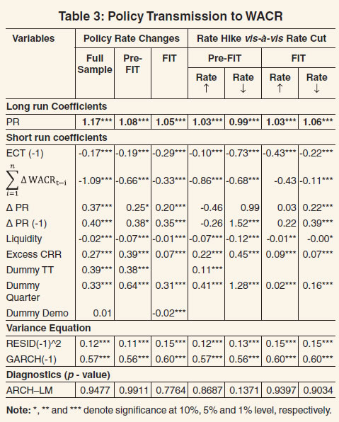 The above findings underscore the need for more proactive liquidity management to achieve monetary marksmanship during the FIT period, considering the institutional features, calendar effects, and market dynamics. Nevertheless, the greater impact of policy announcements on the operating target vis-a-vis shifts in systemic liquidity conditions merits closer scrutiny of market microstructure issues. References: Bollerslev, T. (1986), “Generalized Autoregressive Conditional Heteroskedasticity”, Journal of Econometrics, 31(3), 307-327. Pesaran, M., Y. Shin & R. Smith (2001), “Bounds Testing Approaches to the Analysis of Level Relationships”, Journal of Applied Econometrics, 16, 289–326. | Transmission to Broader Market Segments IV.29 During the FIT period prior to COVID-19 outbreak (October 2016 to March 10, 2020), monetary transmission has been full and reasonably swift across the money market, the private corporate bond market and the government securities market. In the money market, interest rates on 3-month certificates of deposit (CDs), 3-month commercial papers (CPs) and 91-day Treasury bills (T-Bills) moved in sync with the policy rate, lowering funding and working capital costs. As against the cumulative reduction of 135 bps in the policy rate during FIT, the yield on 3-month T-Bills declined by 165 bps, while the yield on 3-month CPs issued by non-banking finance companies (NBFCs) declined by 117 bps (Table IV.8). Transmission to the government securities market and the corporate bond market, however, was less than complete. Since February 2019, improved transmission was facilitated by several liquidity augmenting measures (both conventional and unconventional) announced by the RBI. | Table IV.8: Policy Transmission to Financial Market Segments | | | FIT (Per cent) | Variation during FIT
(bps) | | 03-Oct 2016 | 06-Jun 2018 | 06-Feb 2019 | 10-Mar 2020 | | I. Policy Repo Rate | 6.50 | 6.25 | 6.50 | 5.15 | -135 | | II. Money Market | | (i) WACR | 6.39 | 5.88 | 6.42 | 4.96 | -143 | | (ii) Tri-party Repo | 6.19 | 5.71 | 6.34 | 4.86 | -133 | | (iii) Market Repo | 6.38 | 5.78 | 6.33 | 4.86 | -152 | | (iv) 3-month T-bill | 6.45 | 6.51 | 6.56 | 4.80 | -165 | | (v) 3-month CD | 6.61 | 7.54 | 7.17 | 5.23 | -138 | | (vi) 3-month CP (NBFCs) | 7.00 | 8.18 | 7.78 | 5.83 | -117 | | III. Corporate Bond Market | | (i) AAA -5-year | 7.52 | 8.70 | 8.55 | 6.53 | -99 | | (ii) AAA-10-year | 7.62 | 8.74 | 8.67 | 7.13 | -49 | | IV. G-sec Market | | (i) 5-year G-sec | 6.77 | 8.02 | 7.32 | 5.93 | -84 | | (ii) 10-year G-sec | 6.77 | 7.92 | 7.36 | 6.07 | -70 | | Source: RBI; Bloomberg. | IV.30 Empirical evidence suggests differential impact of monetary policy announcements on various market segments (Box IV.4). Box IV.4
Transmission to Other Markets Based on daily data spanning October 2016-March 2020, monetary policy surprises are calculated as the change in the one-month overnight indexed swap (OIS) on the monetary policy announcement days (Kamber and Mohanty 2018, Mathur and Sengupta 2019). The OIS instruments are forward looking and take into account all the anticipated monetary policy changes until the policy announcement date. Any change in the one-month OIS rate on the monetary policy announcement day reflects the unanticipated component or surprise element of monetary policy.18 The transmission of monetary policy surprises and its impact on various markets (10-year G-sec yield, 5-year AAA corporate bond yield, INRUSD exchange rate and Nifty) is examined through the local projection method (Jorda, 2005), which measures the magnitude of monetary policy surprises on financial markets through the following equation  where h = 1, …, 12 days. The coefficient βh represents the average impact of a monetary policy surprise on the variable of interest h days after the shock. Δyt+h is the change in the dependent variable (10-year G-sec yield, 5-year AAA yield, INRUSD exchange rate return and Nifty return) measured over a one-day window at different horizons of h. Equation 1 is estimated separately for each of the markets as the dependent variable and the coefficients of monetary policy surprises are reported as the results of the cumulative impulse response function with 90 per cent confidence interval. A robustness check of the results undertaken through statistical identification methods (Rigobon, 2003) corroborate the findings. The monetary policy surprise is immediately transmitted to G-sec and corporate bond yields with persistent impact. The cumulative impulse response function implies that a one per cent monetary policy surprise (increase) on announcement day hardens 10-year G- sec and AAA 5-year corporate bond yields, cumulatively on average, by about 0.98 per cent and 0.9 per cent, respectively, over the next 12 days (Chart 1). The impact on the forex and stock market, however, is not significant.19 References: Jorda O. (2005), “Estimation and Inference of Impulse Responses by Local Projections”, American Economic Review, 95, 161-182. Kamber G., and M.S. Mohanty (2018), “Do Interest Rates Play a Major Role in Monetary Policy Transmission in China?”, BIS Working Papers No. 714, Bank for International Settlements. Mathur A., and R. Sengupta (2019), “Analysing Monetary Policy Statements of the Reserve Bank of India,” IHEID Working Papers 08-2019, Economics Section, The Graduate Institute of International Studies. Prabu E. A., and P., Ray (2019), “Monetary Policy Transmission in Financial Markets”, Economic and Political Weekly 54.13, pp. 68–74. Rigobon R. (2003), “Identification Through Heteroskedasticity”, The Review of Economics and Statistics, Vol. 85, pp. 777–792. | Credit Market Transmission IV.31 Following the deregulation of lending rates of scheduled commercial banks (SCBs) in October 1994, the Reserve Bank mandated the benchmarking of rupee loans pricing by banks, beginning with the prime lending rate (PLR) regime. The PLR regime (October 1994 to March 2003) was followed by the benchmark PLR (BPLR) regime (April 2003 to June 2010) and the base rate regime (July 2010 to March 2016).17 These benchmarks – based on internal parameters of balance sheets such as the cost of funds and operating costs – were bank-specific. Although the Reserve Bank had introduced external benchmark-based lending in 2000 to run in parallel, banks almost invariably offered loans based on the internal benchmark, arguing that external benchmarks do not reflect cost of funds (RBI, 2018a). The introduction of the marginal cost of funds-based lending rate (MCLR) regime – the latest internal benchmark introduced by the RBI in April 2016 – almost coincided with the adoption of FIT (Table IV.9). In case of the internal benchmark-based pricing of loans, transmission from the policy rate to bank lending rates is indirect, since lending rates are determined on a cost-plus basis. This creates a wedge in the pricing of bank credit, unlike in the determination of money market rates and bond market yields where transmission is direct (Kavediya and Pattanaik, 2016). In recognition of this asymmetry, the RBI mandated the introduction of an external benchmark system of lending rates for select sectors three years into the FIT regime in October 2019.20 | Table IV.9: Transmission from Repo Rate to Banks’ Deposit and Lending Interest Rates | | (Basis points) | | | Repo rate | Median Term Deposit Rate | WADTDR | WALR - Outstanding Rupee Loans | WALR - Fresh Rupee Loans | | Pre- FIT | Apr 2004 – Sep 2008 | 300 | 229 | 253 | -23 | - | | Oct 2008 – Feb 2010 | -425 | -227 | -174 | -181 | - | | Mar 2010 -June 2010 | 50 | 0 | - | - | - | | July 2010 - Mar 2012 | 325 | 226 | 222 | 203 | - | | Apr 2012 – June 2013 | -125 | -4 | -46 | -44 | - | | July 2013 - Dec 2014 | 75 | 7 | -9 | -28 | 5 | | Jan 2015 – Sep 2016 | -150 | -96 | -123 | -67 | -110 | | FIT | Oct 2016- May 2018 | -50 | -62 | -70 | -92 | -95 | | June 2018 – Jan 2019 | 50 | 16 | 20 | 2 | 57 | | Feb 2019 – Mar 2020 | -135* | -48 | -53 | -27 | -115 | *: The 75-bps policy rate cut on March 27, 2020 is not included.
WALR: Weighted Average Lending Rate; WADTDR: Weighted Average Domestic Term Deposit Rate.
Source: RBI. | Transmission under FIT IV.32 The MCLR system introduced in April 2016 endured only for a brief eight-month period of tight monetary policy (June 2018-January 2019), preceded and followed by easing cycles. Transmission to deposit and lending interest rates remained muted during the initial months of FIT, but it gained traction post-demonetisation (November 2016 to November 2017), resulting from an unprecedented influx of low cost current account and savings account (CASA) deposits into the banking system which, in turn, encouragedbanks to lower their term deposit rates.21 The introduction of external benchmarking of lending rates for retail and micro and small enterprises (MSEs) loans in October 2019 and syncing of liquidity in the financial system with the stance of monetary policy were noteworthy reform measures in support of transmission during the FIT period. IV.33 It is estimated that a policy rate change impacts the weighted average lending rate (WALR) on fresh rupee loans sanctioned by commercial banks with a lag of 2 months and the impact peaks in 3 months - the impact used to peak in 4 monthsin the pre-FIT period.22 IV.34 The pass through to WALR on fresh rupee loans improved in the FIT period vis-à-vis pre-FIT in response to the policy rate tightening (Table IV.9). A reduction in the policy repo rate, however, had noticeable impact on lending rates duringboth regimes.23 IV.35 There is evidence of asymmetry in pass-through of policy repo rate changes to banks’ lending and term deposit rates. Transmission is uneven across bank groups as well as across monetary policy cycles (Singh, 2011; Das, 2015; Khundrakpam, 2017), and usually higher for weighted average outstanding domestic term deposit rates (DR) and weighted average lending rates (WALRs) on fresh rupee loans (LR-F) vis-à-vis WALRs on outstanding rupee loans (LR-O) over different policy cycles (Table IV.10). Sensitivity of Output and Inflation to Monetary Policy IV.36 Since monetary transmission is subject to long, variable and uncertain lags, most IT central banks have adopted a period in the range of 12-24 months as their policy horizon (Bank of England, 1999; European Central Bank, 2010). An analysis of empirical work reported in the literature suggests that the average transmission lag is 29 months, and the maximum reduction in prices is, on average, 0.9 per cent following a one percentage point hike in the policy rate (Havranekand Rusnak, 2013).24 Transmission lags are longer in developed economies (26 to 51 months) than in post-transition economies (11 to 20 months). The difference in the speed of adjustment between developed and post-transition economies has been attributed to the degree of financial development: greater financial development is associated with slower transmission, as developed financial institutions have more opportunities to hedge against surprises in monetary policy actions. In developing countries, however, an underdeveloped financial market impedes transmission (Mishra et al., 2012). It appears that it is not the stage of development of financial markets per se, but it is the choice of an appropriate monetary regime that is more important in determining the strength of monetary transmission (Marques et al., 2020). IV.37 A survey of the empirical literature across countries shows that monetary policy impacts output with a lag of up to 12 months and inflation with a lag of up to 39 months and monetary policy impulses persist up to 60 months and even beyond for some countries. The lagged impact is sensitive to sample period, assumptions and methodology adopted for empirical analysis (Annex IV.2). IV.38 For India, empirical results from estimating New Keynesian models with inflation measured by the WPI indicate that in response to policy tightening, output starts contracting after three quarters and reaches its trough after one more quarter before gradually returning to its baseline. Inflation responds after seven quarters of the shock and the maximum impact is felt after 10 quarters(Patra and Kapur, 2012).25 When data on CPI are used, the transmission of a policy rate increase to headline CPI inflation peaks after 4 years (Kapur, 2018). In the QPM, the peak impact of monetary policy tightening on CPI inflation occurs after 10 quarters (Benes et al., 2016). There is a consensus that the interest rate channel is the strongest conduit of transmission, followed by thecredit channel.26 | Table IV.10: Transmission across Bank Groups – Tightening and Easing Policy Cycles | | (Basis points) | | Policy Cycle | Repo Rate | Public Sector Banks | Private Sector Banks | Foreign Banks | SCBs | | DR | LR-O | LR-F | DR | LR-O | LR-F | DR | LR-O | LR-F | DR | LR-O | LR-F | | Oct 16 - May 18 | -50 | -77 | -95 | -107 | -54 | -91 | -108 | -58 | -74 | -59 | -70 | -92 | -95 | | June 18 – Jan 19 | 50 | 13 | -32 | 37 | 29 | 53 | 78 | 60 | 35 | 75 | 20 | 2 | 57 | | Feb 19 – Mar 20 | -135 | -42 | -35 | -83 | -70 | -11 | -140 | -139 | -89 | -135 | -53 | -27 | -115 | DR: Weighted average domestic rupee term deposit rate; LR-O: Weighted average lending rate on outstanding rupee loans; LR-F: Weighted average lending rate on fresh rupee loans sanctioned by banks.
Source: RBI. | 3. Fine-tuning the Operating Procedure and Transmission Channels IV.39 The lessons from the implementation of monetary policy under FIT juxtaposed with the contemporaneous country experience points to the scope for several refinements in the operating framework and market infrastructure which can potentially improve the efficiency of monetary policy in the transmission of signals across the term structure of interest rates and the spectrum of markets in the economy. It is important to delineate, however, what works and, therefore, need not be fixed. Uncollateralised vis-à-vis collateralised rate as the operating target IV.40 The WACR should continue as the operating target of monetary policy. The gradual shrinkage in the share of the call money market in total money market turnover is mirrored in the experiences of countries across the world and this has not been deemed inimical to the integrity of the call money rate as an operating target by the majority of central banks, although a few viz., Brazil, Canada, Mexico, Switzerland choose the collateralised rate as the operating target (Annex IV.1). Moreover, collateralised segments of the money market are also populated by non-bank and unregulated participants whose actions may not be consistent with the monetary policy stance or amenable to the central bank’s regulatory control. Technically, the Reserve Bank can exert countervailing influence over them by its power to create reserves, but this may prove to be inefficient and costly in terms of the volumes of liquidity that has to be injected or withdrawn and the frictions encountered in the interface with the Reserve Bank’s collateral policy. Corridor Play, Marksmanship and MPC’s Mandate IV.41 As stated earlier, the FIT period was marked by the WACR trading with a pronounced downward bias vis-à-vis the policy repo rate. Moreover, the corridor was made asymmetric on March 27, 2020 by reducing the reverse repo rate by an additional 15 bps over and above the75 bps reduction in the repo and the MSF rate.27 Cumulatively, these two factors have resulted in the WACR getting closely aligned with the reverse repo rate (Chart IV.6). In this context, it has been argued in some section of the media and by a few analysts that by undertaking unilateral reductions in the reverse repo rate not in proportion to the repo rate, the Reserve Bank has solely appropriated for itself the task of monetary policy decision making. 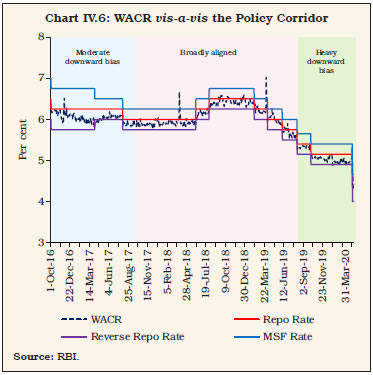 IV.42 The amended RBI Act entails that the MPC shall determine the policy rate required to achieve the inflation target. It also defines the policy rate as the repo rate under the LAF. The operating procedure of monetary policy is guided by the objective of aligning the operating target of monetary policy – the WACR – to the repo rate through active liquidity management, consistent with the stance of monetary policy (RBI, 2015). Day to day liquidity management function is solely in the domain of the Reserve Bank. During normal times, the reverse repo rate and the MSF rate move in sync with repo rate changes as they are pegged to the repo rate in an equidistant manner under a symmetric corridor. In exceptional times, however, the corridor itself becomes an instrument for managing liquidity conditions. As the marginal standing facility and the fixed rate reverse repo windows are essentially instruments of liquidity management, they are in the remit of the Reserve Bank. In its endeavour to achieve the policy rate voted upon by the MPC, decisions involving a change in the reverse repo rate and the MSF rate and announcements thereof may be shifted out of the MPC resolution to the Reserve Bank’s Statement on Developmental and Regulatory Policies. The RBI may also clarify for the purpose of anchoring expectations that in normal times it will work with a symmetrical corridor with the MSF rate and the fixed rate reverse repo rate at pre-specified alignment with the policy repo rate and that it reserves the option of operating with an asymmetric LAF corridor in exceptional times. IV.43 When the MPC decided to adopt an accommodative stance of policy in June 2019, the Reserve Bank, in pursuance, ensured that systemic liquidity migrated from deficit to surplus by injecting large amounts of durable liquidity into the banking system through forex operations and OMO purchases and later through LTROs and TLTROs. In the absence of adequate opportunities for productive deployment of funds, surplus liquidity was parked by banks with the RBI under the reverse repo window. In this milieu, the reduction in the reverse repo rate was aimed at discouraging banks from passively parking surplus liquidity and explore lending opportunities amidst the nation-wide lockdown. The downside risk that emerged was that collateralised money markets traded, on average, 49-58 bps lower than the reverse repo rate. Term premia on instruments such as treasury bills, CPs and CDs moderated sharply – their interest rates trading below the overnight fixed rate reverse repo – posing threats to financial stability. Given this backdrop, it needs to be recognised that the asymmetric corridor is a temporary measure which will be reversed once normalcy is restored and that it would be misleading to interpret a crisis-induced measure as an attempt to weaken the MPC. IV.44 In view of the above, clarity of roles and responsibilities is clearly warranted to preserve the public’s credibility in monetary policy procedures so that expectations are anchored to this goal and intent. Consistency of actions with the publicly communicated stance would preserve and enhance transparency under the FIT framework. Narrow versus Wide Corridor IV.45 At the start of FIT in India, the Reserve Bank indicated a preference for narrowing the LAF corridor in keeping with peer country experiences with a view to honing monetary marksmanship in aligning the WACR closely with the policy repo rate (Patra et. al, 2016; RBI, 2016). While a narrow corridor lowers volatility in the operating target, it dis-incentivises the inter-bank market, resulting in the central bank emerging as the sole counterparty. In contrast, a wide corridor entails costlier central bank liquidity facilities but encourages active inter-bank trading and the development of the market segments, participants and products that continuously price and transfer various kinds of risks, but at the cost of tolerating higher volatility (Bindseil and Jablecki, 2011), which can amplify to a point at which it impedes monetary transmission. Therefore, the trade-off between low volatility and market buoyancy has to be keenly weighed before deciding on the appropriate width of the corridor. It is pertinent to note that ultra-low volatility (a very stable rate) is not particularly helpful for market making as contrasting views are necessary to spur market activity. As the pandemic recedes, exceptional measures are wound down and normalcy is restored, it is envisaged that the pre-pandemic LAF corridor of +/-25 bps may be gradually reinstated. At that stage, it may be appropriate to fully resume the revised liquidityframework laid out in February 202028 (Box IV.1) with 14-day repo/ reverse repo auctions as the main liquidity operation with cut-offs finely aligned with the policy rate to secure marksmanship. Capital flows and Liquidity Management IV.46 Large swings in capital flows can undermine the stance of monetary policy and pose challenges for liquidity management, as Chapter V dwells upon in detail. Forex market intervention by the Reserve Bank is aimed at curbing excessive volatility and discourage disruptive speculative activities in the foreign exchange market: large-scale capital outflows necessitate forex sales to avoid high volatility of the domestic currency on the downside, while a deluge of inflows warrants forex purchases to prevent volatility on the upside. More pressing are the resulting liquidity consequences of these interventions (Raj et al., 2018). Forward interventions may be liquidity neutral but by imparting pressure on the short-term interest rates, they can produce a similar outcome of contravening the policy stance. Forex purchases, by expanding domestic liquidity, exert downward pressure on money market rates which may be at variance with the stated policy stance. Moreover, in situations of exceptional liquidity glut, the traditional instrument viz., OMO sales have limitations in terms of the availability of adequate securities in the Reserve Bank’s portfolio. Furthermore, the reverse repo window, being a short-term instrument whose impact gets quickly reversed, cannot be an effective sterilisation tool for durable liquidity flows. In times of extreme liquidity tightness, an analogous constraint emerges in the form of the finite stock of excess statutory liquidity ratio (SLR) securities held by banks, which can be used as collateral under the LAF. With the MSF acting as a safety valve on the injection side, it is necessary to impart symmetry to the LAF by providing for a special facility on the absorption side. IV.47 In this context, the standing deposit facility (SDF) announced in the Union Budget 2018-19 and notified in April 2018, which is unencumbered and unconstrained regarding availability of securities, can be activated. The design of the SDF in terms of the appropriate interest rate and the conditions under which it is triggered, however, merits closer scrutiny since it would act as an additional floor to interest rates, beside the existing reverse repo rate. If the reverse repo facility has to be kept active or a potent tool of liquidity management, the interest rate on SDF must be lower than the reverse repo rate. Thus, the SDF will ensure that tail events such as a deluge of capital inflows do not threaten financial stability without the need to take recourse to instruments outside the Reserve Bank’s toolkit (eg., MSS). In that sense, the SDF needs to be regarded as a tool for ensuring financial stability in addition to its role in liquidity management (RBI, 2018b). Improving Liquidity Assessment and Communication IV.48 With the introduction of the 14-day variable rate repo as the main liquidity management tool synchronised with the reserve maintenance period, a more accurate assessment of liquidity is critical for both the Reserve Bank and the commercial banks, combining top-down methodologies and bottom-up approaches. From the Reserve Bank’s standpoint, resources have to be invested into availability of information on a more concurrent basis and more precise forecasts of autonomous factors such as currency demand, government cash balances and forex flows for a systematic liquidity assessment over the reserve maintenance fortnight. Illustratively, government cash balances are available to the liquidity forecaster with a lag of one day and currency in circulation with a lag of one week whereas they should be available on the same day and even intra-day for frictional liquidity management operations. As committed to in the revised liquidity management framework announced in February 2020, the Reserve Bank’s assessment of autonomous liquidity in an aggregated manner could be made available in the public domain on an ex ante daily / fortnightly basis as an incentive mechanism for improving the quality of forecasts. IV.49 For commercial banks, refining intra-fortnight cash flow projections remains a major challenge. The incentive structure for commercial banks to improve the quality and precision of bottom-up forecast could take the form of a reporting requirement on a pre-set frequency which the Reserve Bank, in turn, can aggregate and release in public domain along with its own assessment / forecasts. IV.50 Active liquidity management also presages the need for operations as needed in the form of two-way OMOs (both purchases and sales), forex operations (both spot and forward) and repo/ reverse repo of various tenors so that quantity modulation occurs seamlessly and persisting liquidity gaps / overhangs, as under the FIT, are avoided. Such gaps / overhangs often lead to large deviation of the operating target from the policy rate necessitating increased intervention by the central bank in the money market thereby hindering efficient price discovery and market development. Alongside, the frequency of fine-tuning operations should be minimised and confined to short tenors which are easily reversible so as not to overwhelm durable liquidity operations. Overall, the success of liquidity management in terms of its objectives hinges around clear and transparent communication of the central bank’s intentions followed up by credible actions resulting in desirable outcomes that are consistent with the publicly communicated stance. Synchronising Market Timings IV.51 Synchronicity in market timings across all products and funding markets is necessary to ensure that they complement each other by avoiding unanticipated frictions. Asynchronous market closure timings across different money market segments, high trading intensity in early hours and market timings not in sync with settlement timings often impact WACR trading disproportionately towards the end of the day. Specifically, the first hour of trading in the call money market usually accounts for bulk of the day’s volume as most of the market participants are unable to assess their cash-flow position for the day in the absence of a robust liquidity forecasting framework. As a result, late hour demand supply mismatches reflect in volatile call rates. Moreover, the absence of uniform market hours across all money market segments (Table IV.11), which are not in sync with real time gross settlement (RTGS) timings often have a destabilising impact on the WACR towards the market’s closure as cooperative banks enter the market to lend at cheaper rates. Therefore, standardising operational timings across market segments would reinforce the sanctity of the WACR as the operating target. | Table IV.11: Market Timings | | Market | Trading System | Settlement type | Entities | Market Timings | | Open | Close | | Call Money market | NDS-Call | T+0
T+1 (Notice/ Term) | All Entities | 9.00 AM | 5.00 PM | | Tri-party Repo in Government securities | TREPS | T+0 | Entities settling funds at RBI | 9.00 AM | 3.00 PM | | | | | Entities settling funds at Settlement Bank | 9.00 AM | 2.30 PM | | Tri-party Repo in Government securities | TREPS | T+1 | Entities settling funds at RBI | 9.00 AM | 5.00 PM | | | | T+1 | Entities settling funds at Settlement Bank | 9.00 AM | 5.00 PM | | Market Repo in Government Securities | CROMS | T+0 | All Entities | 9.00 AM | 2.30 PM | | Market Repo in Government Securities | CROMS | T+1 | All Entities | 9.00 AM | 5.00 PM | | Repo in Corporate Bond (reporting) | F-TRAC | T+0 | All Entities | 9.00 AM | 6.00 PM | | Repo in Corporate Bond (reporting) | F-TRAC | T+1 | All Entities | 9.00 AM | 6.00 PM | | Government Securities (Central Government Securities, State Development Loans and Treasury Bills) | NDS-OM | T+0 | All Entities | 9.00 AM | 2:30 PM | | Government Securities (Central Government Securities, State Development Loans and Treasury Bills) | NDS-OM | T+1 | All Entities | 9.00 AM | 5.00 PM | Note: In order to minimise the risks of contagion from COVID-19 and to ensure safety of personnel, trading hours for various markets were curtailed effective April 7, 2020.
Source: RBI. | IV.52 Among Asian economies, interbank money markets are open till about 4-6:30 pm (local time) in Indonesia, Malaysia, South Korea and Hong Kong. The cut-off timings of payment systems relating to customer transactions is before closure of money markets in many of these jurisdictions; however, retail payment systems remain open post closure of money markets in China, Thailand and Vietnam. IV.53 Synchronous operational timings in the money market is vital so that participants have access to collateralised / uncollateralised funding as per their requirements. It also alleviates pressure on any segment that remains operational after the closure of other segments, as is the case in funding markets. Different settlement mechanisms for collateralised (market repo and TREPS) segments and uncollateralised (call) segment, however, pose challenges in aligning timings. The settlement of transactions in market repo and TREPS takes place along with secondary market transactions in securities segment. Multilateral netting of funds and securities results in high degree of netting benefits for market participants in terms of liquidity requirement. Furthermore, sufficient time is also required to facilitate repayment of intra-day credit lines availed by market participants from banks after completion of securities settlement. Availability of large value payment systems, such as RTGS, facilitates efficient functioning of the collateralised funding markets. IV.54 Finally, synchronised timing is also necessary from the viewpoint of meeting intra-day liquidity challenges due to sequencing of settlements. For instance, primary auctions and OMOs settle at about mid-day while settlement of securities are towards the end of the day. This sequencing of settlements may increase the intraday liquidity needs of the system as some market participants may have payable position in one settlement and receivable in another. Hence, primary auction/OMO settlement may be conducted later in the day. This would not only improve the netting efficiency but also help in reducing the overall liquidity requirement (RBI, 2019). Impediments to Transmission IV.55 Monetary transmission in India is delayed and incomplete. Several factors impeded policy transmission to deposit and lending interest rates of banks during the FIT regime (Box IV.5). Policy Measures Undertaken to Improve Transmission in Credit Market IV.56 Keeping in view the drags on transmission, a few initiatives were taken to facilitate transmission in the FIT period. As the experience with the introduction of MCLR regime coinciding with FIT framework did not prove to be satisfactory, the Reserve Bank mandated introduction of external benchmark linked loans for retail and MSE sectors in October 2019; and for medium enterprises, effective April 1, 2020. IV.57 Notably, a cross country survey of interest rate benchmarks adopted by banks reveals that loans linked to external benchmarks constitute a significant share of balance sheets of banks in many countries (Table IV.12). Box IV.5
Impediments to Monetary Policy Transmission during FIT Since the deregulation of interest rates in the early 1990s, the Reserve Bank has made concerted efforts to improve the effectiveness of monetary transmission by refining the process of interest rates setting by banks. Several specific factors, however, continue to impede monetary transmission in the credit market during FIT regime. These include: internal benchmarks for pricing of loans by banks29; distortive interest rate subventions; mismatches in the maturity profile of banks’ assets and liabilities; funding of assets dependent on longer maturity fixed rate retail deposits; loans mostly contracted at floating rates but long maturity profile of deposits at fixed interest rates; rigidity in interest rates on banks’ saving deposits; higher interest rates offered by competing saving instruments such as small saving schemes and debt mutual fund schemes; and deterioration in the asset quality of commercial banks. The lack of transparency in the pricing of loans by NBFCs makes it difficult to assess transmission, let alone address the impediments. 1. The pricing of loans during the post-deregulation period is primarily based on internal – and hence, bank specific – benchmarks that are not conducive to customer awareness and protection. The adoption of FIT in India broadly coincided with the introduction of marginal cost of funds-based lending rate (MCLR) system in April 2016. Banks arbitrarily adjusted their MCLRs and the spread, which impeded transmission of policy rate cuts to borrowers. In this regard, the key findings of the Internal Study Group to review the Working of the MCLR system (Chairman: Dr. Janak Raj) were: (i) large reduction in MCLR was partly offset by some banks by a simultaneous increase in the spread in the form of business strategy premium that lowers the pass-through to lending rates; (ii) some banks did not have any methodology for computing the spread, which was merely treated as a residual arrived at by deducting the MCLR from the actual prevailing lending rate; and (iii) the credit risk element was not applied based on the credit rating of the borrower concerned, but on the historically observed probability of default (PD) and loss given default (LGD) of the credit portfolio/sector concerned. Besides, in the absence of any sunset clause on the base rate, banks were slow in migrating their existing customers to the MCLR regime. It took around four years for the share of loans linked to the base rate to decline to single digit. 2. A major factor that prevents banks from passing the benefits of transmission has been the relatively long maturity profile of term deposits contracted at fixed rates (Chart 1), while loans – though skewed towards the longer-term – are contracted mostly at floating interest rates (72.8 per cent in end-June 2020), resulting in the duration mismatch of banks’ assets and liabilities (Chart 2). 3. Another cause of weak transmission is the rigidity in interest rates on banks’ saving deposits which constitute nearly one-third (around 32 per cent since demonetisation) of aggregate deposits. The median saving deposit rate remained constant for almost six years since its deregulation in October 2011 although the policy cycle moved in either direction (RBI, 2017). It was only after large influx of current account and savings account (CASA) deposits in the banking system on account of demonetisation – entirely unrelated to monetary policy – that major public sector banks, led by the State Bank of India, lowered the interest rate on saving deposits on July 31, 2017 (Chart 3).30 The mandatory introduction of external benchmark linked loans for select sectors has broken the jinx, as it were, in bringing about an end to rigidity in saving deposit rates. 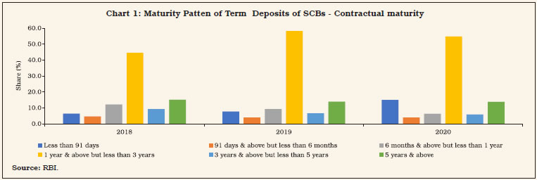 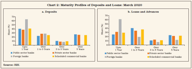 4. The interest rates on small saving schemes are administered by the central government and are linked to the secondary market yields on G-secs of comparable maturities. Although it was decided to set these interest rates on a quarterly basis (with a 4-month lag)31 since April 2016, broadly coinciding with the introduction of the FIT regime, the implementation was half hearted, particularly during the easing cycle. Thus, the actual rates of interest of various small saving instruments were higher than the formula-based rates during Q2:2017-18 to Q4:2017-18 and Q1:2019-20 to Q4:2019-20. For e.g., the administered interest rates on small saving schemes were higher by 81-160 bps as compared with the formula-based rates in Q4: 2019-20 as the government left small saving interest rates unchanged for Q3 and Q4:2019-20, notwithstanding the decline in G-sec yields during the reference period, with implications for monetary transmission. Higher interest rates offered by competing saving instruments such as small saving schemes and debt mutual fund schemes have impeded transmission especially during the easing cycle, although bank deposits have some distinct advantages in the form of stable returns (vis-à-vis mutual fund schemes) and liquidity (vis-à-vis small saving schemes). Besides, small savings are liabilities of the sovereign and are free from credit risk. Banks, therefore, often appeared to be reluctant in the past to reduce interest rates on term deposits in line with the reduction in the policy rate by the Reserve Bank.32 These factors imparted rigidity to the liability side of banks’ balance sheets. 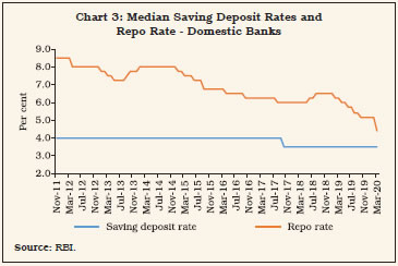 5. The deterioration in the health of the banking sector and the expected loan losses in credit portfolios impacted monetary transmission (John et al., 2018). An increase in credit risk [proxied separately by the gross non-performing assets (NPA) ratio and the stressed assets ratio (NPA plus restructured assets)] impeded monetary transmission through the interest rate channel. Transmission was also hindered through the bank lending channel during the more recent period as credit growth decelerated in response to a sharp deterioration in asset quality (Raj et al., 2020). 6. The relative significance of NBFCs in the financial system has been growing. The share of NBFCs in credit extended by banks and NBFCs increased from 9.5 per cent in March 2008 to 18.6 per cent in March 2020. NBFCs, however, do not follow a uniform methodology in the pricing of loans. While some NBFCs use their own prime lending rates as interest rate benchmarks, others use base rates/MCLRs of banks as external benchmark; a few do not have any interest rate benchmark for their loan pricing. The lack of transparency has resulted in weak transmission of monetary policy in this segment of financial market. 7. Fiscal dominance in policy making has continued to impinge on the efficacy of monetary policy in India (Mitra et al., 2017). Open market operations are employed in the context of large government borrowings crowding out non-food credit extended by banks. The SLR prescription provides a captive market for government securities and helps to artificially suppress the cost of borrowing for the Government, dampening the transmission of interest rate changes across the term structure. Though the SLR regulatory floor has been reduced to 18 per cent of NDTL, banks maintain higher SLR than the prescribed limit (26.4 per cent as at end- March 2020). The excess SLR is LAF eligible, which incentivises banks to maintain excess SLR. In addition, weak demand for credit and risk aversion among banks (including ‘lazy banking’) appear to motivate banks to invest in government securities more than their statutory requirements. In case of weaker banks, particularly those under prompt corrective action (PCA) framework of the RBI, inadequate capital could also constrain lending operations of banks. The Government also influences the monetary policy transmission channel through moral suasion and at times, directives, to banks. The central and state governments offer interest rate subvention to certain sectors, which distorts setting of competitive prices for loans in free market. 8. There is significant presence of informal/semi-formal lending system in India, particularly in rural areas. The cost of borrowing from informal sources is significantly higher than that of borrowing from banks. Thus, the significant presence of informal finance as well as its costs of intermediation can impede the impact of monetary policy on aggregate demand. References: John, J., A.K. Mitra, J. Raj and D.P. Rath (2018), “Asset Quality and Monetary Transmission”, Reserve Bank of India Occasional Papers, Vol 37 (1&2), 35-62. Mitra, P., I. Bhattacharyya, J. John, I. Manna and A. T. George (2017), ‘‘Farm Loan Waivers, Fiscal Deficit and Inflation’’, Mint Street Memo No. 5, Reserve Bank of India. Raj, J., D.P. Rath, P. Mitra & J. John (2020), “Asset Quality and Credit Channel of Monetary Policy Transmission in India: Some Evidence from Bank-level Data”, Reserve Bank of India Working Paper No. 14/2020. RBI (2017), Report of the Internal Study Group to Review the Working of the Marginal Cost of Funds-Based Lending Rate System (Chairman: Dr. Janak Raj), October. | IV.58 An overview of country practices33 on setting of lending and deposit rates suggests that developed economies have typically two benchmark rates – one for retail loans and another for corporate loans. For instance, in the US, the prime rate – normally 3 percentage points higher than the federal funds rate – is usually the benchmark rate for consumer and retail loans; and London Inter-Bank Offered Rate (LIBOR) is the reference rate for corporate loans (and also for longer maturity floating rate mortgages). Similarly, in the UK, the Bank of England’s base rate is a key benchmark rate for consumer and retail loans, while LIBOR is the benchmark for commercial loans. In case of countries such as the US and the UK, the external benchmark rates have evolved out of market practices. In case of China, however, the Chinese central bank i.e., the People’s Bank of China (PBC) appears to goad commercial banks to link their benchmark rate, viz., lending prime rate (LPR) – a reference rate monthly reset by 18 banks – to the interest rate of one of its main tools for managing longer-term liquidity in the banking system, which serves as a guide for the LPR (Reuters, 2020). | Table IV.12: Proportion of Loans linked to Internal and External Benchmarks | | (Per cent) | | Country | Internal | External | Total | | Thailand | 95 | 5 | 100 | | Indonesia | 90 | 10 | 100 | | Switzerland | 80 | 20 | 100 | | Turkey | 55 | 45 | 100 | | Malaysia | 45 | 55 | 100 | | United Kingdom | 45 | 55 | 100 | | Taiwan | 40 | 60 | 100 | | Singapore | 30 | 70 | 100 | | South Korea | 10 | 90 | 100 | | China | 0 | 100 | 100 | | Source: Credit Suisse Research, HDFC Bank (Acharya, 2020). | IV.59 The shift to external benchmark for select sectors has ushered in transparency in interest rate setting by banks for those sectors; facilitated product comparison (say, lending rate on housing loans) across banks; ensured customer protection; and greatly facilitated transmission. The transmission from the policy rate to the lending rate is more direct than under internal benchmarks (with most banks having adopted the policy repo rate as the desired benchmark). Banks would need to reset the lending rate at least once in three months for existing borrowers to reflect the change in the benchmark rate on a 1-1 basis, speeding up transmission from the MCLR regime, where loans are typically reset on an annualfrequency (Mitra and Chattopadhyay, 2020).34 Besides, the spread would not be frequently/ arbitrarily revised from time to time defeating the purpose of having a benchmark; instead, it will be subject to review once in 3 years (unless there is a credit event). IV.60 Is the mandatory prescription of an external benchmark by the RBI tantamount to re-regulation through the back door? The element of regulation is, in fact, only to the extent of prescription of an external benchmark in respect of floating rate loans, as opposed to an internal benchmark or having no benchmark at all. Prescribing external benchmark was necessitated by the fact that internal benchmarks lacked transparency and were open to manipulation by banks (RBI, 2017). Besides, under the internal benchmarking regime, both the benchmark rate as also its quantum of change differ from one bank to another, making it difficult for the prospective borrower to compare the interest rate of a loan product across banks andover time.35 Second, even while recommending an external benchmark, banks were given the choice of selection among any one of the benchmarks published by FBIL and the policy repo rate, even though most banks, of their own volition, have preferred to opt for the latter. Third and most importantly, banks are completely free to determine the spread over the external benchmark at the time of loan sanction, based on their commercial judgement; and hence, the lending rate is freelydetermined by the operation of market forces.36 Banks also have the freedom to load extra cost of funding or any other costs such as operating costs in the spread at the time of sanctioning of the loans. Having once fixed the spread (and hence, the lending rate), banks are permitted to revise the spread only once in three years except for a major credit event. If the spread remained variable just as the benchmark, the purpose of benchmarking would have got defeated, which is that lending rate ought to change only when the benchmark changes. This stipulation is aimed at safeguarding the interests of the borrowers through the entire loan repayment period since the experience with the internal benchmark regimes has been that banks do not always pass on the entire benefits of the lower benchmark rate to their old borrowers even while passing on the entire benefit of lower interest rate environment to the prospective customers to gain market share. The external benchmark regime thus aims at balancing the interests of the lender with that of the borrower. IV.61 The hallmark of FIT regime is transparency, which is also applicable to the external benchmarking regime. Undoubtedly, it would have been ideal had an external benchmark emerged automatically in a market driven process. This, however, was unlikely given the limited depth of money markets, thereby requiring handholding from the Reserve Bank to facilitate emergence of the benchmark as was envisaged by the Expert Committee to Revise and Strengthen the Monetary Policy Framework (RBI, 2014) and the Internal Study Group to Review the Working of the MCLR System (RBI, 2017); this is also consistent with the developmental role played by central banks, including from advanced economies, particularly following the LIBOR episode. IV.62 Introduction of external benchmark for the pricing of loans did not inconvenience banks as the cost of funds is now more closely aligned to the policy rate with the spread over repo rate declining from 217 bps in March 2012 to 11 bps inMarch 2020 (Chart IV.7).37 Improving Transmission in the Credit Market IV.63 Efficient monetary transmission in a bank-dominated financial system implies that deposit and lending rates change in quick time in line with the policy rate to meet the monetary policy objective as laid down in the RBI Act. Addressing the impediments to transmission would facilitate adherence to the inflation targeting framework. 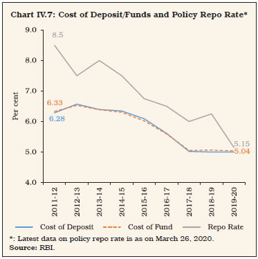 IV.64 If interest rates in the banking system – unlike the money and bond market rates – do not change in line with the policy rate, the monetary authority of a bank-dominated financial system has to either persist with the policy rate for longer to steer growth towards its potential and inflation towards its target; or change the policy rate by much more than would have been the case if interest rates in the credit market moved in tandem with the policy rate. When there is a wide divergence in the movement between money and bond market interest rates on the one hand and credit market on the other, suboptimal allocation of resources may result from imperfect price signals, impacting growth and price stability. If the external benchmarking regime is made applicable to the entire commercial banking sector, not only will it improve monetary transmission, but also indirectly contribute to monetary and financial stability (Acharya, 2020). Broadening and Deepening Interest Rate Derivatives Market IV.65 Globally, one of the major tools of managing the duration mismatches between assets and liabilities of banks is through recourse to interest rate derivatives. In India, interest rate derivative markets have grown but have remained limited to one product – the overnight indexed swap (OIS) – and to a small set of market participants (Das, 2020a). In India, there appears to be a chicken and egg problem between the demand and supply sides that restrict participation and limit transactions. A necessary push from the Reserve Bank can break this logjam: the progressive linking of loans to all sectors to one of the external benchmarks currently prescribed for personal and MSME loans for pricing of loans would likely provide a fillip to the development of the derivatives market from the demand side. This, in turn, is expected to provide the necessary impetus to the supply of derivatives products, resulting in an optimal distribution of risk among those who are willing and able to manage without adding to the risks to the financial system as a whole. Linking Deposits to External Benchmarks IV.66 Recourse to derivatives products apart, banks can voluntarily link their liabilities (deposits) to external benchmark rates. To begin with, the interest rates on bulk deposits of high net-worth individuals (HNIs) and corporates who are better equipped to handle interest rate risk than retail depositors, could be linked to external benchmark. This will further facilitate the alignment of banks’ cost of funds with market rates. Migrating Old Loans to External Benchmarks IV.67 The success of the new regime in interest rate setting by banks for better monetary transmission would depend on how quickly and efficiently banks migrate their existing borrowers from the old regime to the new one. Wider publicity may be accorded among borrowers, particularly retail borrowers, about the merits of external benchmarking system through various channels, including in the form of FAQs in layperson language. Improving Disclosure Practices of Banks IV.68 The disclosure practices of banks on lending rates charged by them have room for improvement. In the lines of the recommendations of the Internal Study Group to review the working of the MCLR (RBI, 2017), banks may display prominently in their websites the base rate/MCLR (tenor-wise), the benchmark chosen for external benchmark and the minimum and the maximum spread on loans for each sector separately for loans linked to the base rate, the MCLR and the external benchmark. Information on the spread charged to various categories of borrowers including the credit risk premia and the criteria for levying credit risk premia should be made available on request to the borrowers, including the prospective borrowers. The Indian Banks’ Association (IBA) could disseminate consolidated bank-wise information on its website to enable customers to easily compare the lending rates across banks for various sectors. Aligning Interest Rate Setting Processes of Banks with NBFCs IV.69 For effective monetary policy transmission to the financial intermediaries and ultimately to the real economy, it is necessary that the interest rate setting processes of NBFCs are aligned with those of banks (Acharya, 2020). The external benchmark system could be mandatory for NBFCs as well as housing finance companies (HFCs) for pricing their loans. The harmonisation of lending rates across banks and NBFCs in terms of benchmarks, fixation of spread and the periodicity of interest rate reset would facilitate effective transmission of monetary policy across the entire spectrum of financial intermediaries. Revising Interest Rates on Small Savings at Quarterly Intervals IV.70 To facilitate better transmission, the government should revise interest rates on the various small savings schemes every quarter in line with the well-defined formula as announced by the government in its Press Release dated February 16, 2016. Harnessing FinTechs for Improving Transmission IV.71 The new financial technologies (FinTech) are bringing about an unprecedented change in the financial sector globally; India is no exception. Electronic money (including central bank digital currency), peer to peer lending, crowd funding platform and distributed ledger technology have the potential to transform the financial landscape in the near future (Leong and Sung, 2018). FinTechs would reduce transaction costs among counterparties; provide transparency with simpler products; and increase efficiency (Curran, 2016). FinTechs would be the vehicle to reach customers who are outside the pale of the financial system thereby promoting financial inclusion. In India, FinTechs could function as the fourth segment of the Indian financial system, alongside large banks; mid-sized banks including niche banks; and small finance banks, regional rural banks and cooperative banks (Das, 2020b). IV.72 The role of FinTechs in improving monetary transmission is well recognised in the literature (Bernoth et al., 2017). A light touch regulation for FinTechs can result in regulatory arbitrage vis-à-vis banks, enabling FinTechs to better transmit monetary policy signals than capital constrainedbanks through the bank capital channel.38 Given their nature of operations, FinTechs are more likely to pass on the rate hikes to their customers, facilitating transmission through the lending channel (Bolton et al., 2016). Further, there is an overall strengthening effect of non-bank finance on monetary policy transmission, particularly through the risk-taking channel (IMF, 2016). IV.73 In India, literature on the role played by FinTechs in monetary transmission is scanty. FinTech firms issue loans to SMEs. The rate of interest charged to small businesses ranges between 16 to 27 per cent (Faridi, 2020). This reflects the high cost of borrowing by FinTechs from banks and high-risk premia assigned by FinTechs. Going forward, FinTechs may be required to better manage the risk through use of derivatives and reduce their cost of borrowings for on-lending to retail borrowers at lower rates of interest. IV.74 The push from FinTechs would likely prompt banks and NBFCs in India to adopt financial technology, which, by reducing the cost of intermediation, can bring the hitherto unbanked households and firms within the ambit of formal finance, while facilitating economy-wide monetary transmission. FinTech’s growth will potentially intensify financial sector competition and cause the market to become more sensitive in its response to policy rate changes, which would improve monetary policy transmission. Opportunities and Challenges with CBDC IV.75 Several countries have been toying with the idea of launching central bank digitalcurrency (CBDC) in some form or the other.39 The attractiveness of CBDC stems from its digital feature as well as from being a sovereign liability. CBDC can be designed to promote non-anonymity at the individual level, monitor transactions, promote financial inclusion by direct benefit fiscal transfer, pumping central bank ‘helicopter money’ and even direct public consumption to a select basket of goods and services to increase aggregate demand and social welfare, thereby acting as a direct instrument of monetary transmission. Besides, an interest-bearing CBDC can increase the economy’s response to changes in the policy rate. In advanced economies with low growth and inflation and facing the constraint of “zero lower bound”, CBDC can help countries overcome the constraint with the monetary authority offering negative nominal interest rates to its holders. IV.76 In emerging markets facing large scale capital inflows, CBDC can act as an instrument of sterilisation, alleviating the constraint that a finite stock of government securities in central bank balance sheet poses. A standing deposit facility (SDF) can also play a similar role, but CBDC, if designed to cater to not only wholesale institutions, but also retail individuals, can directly improve and fasten transmission. IV.77 CBDC is, however, not an unmixed blessing – it poses a risk of disintermediation of the banking system, more so if the commercial banking system is perceived to be fragile. The public can convert their CASA deposits with banks into CBDC, thereby raising the cost of bank-based financial intermediation with implications for growth and financial stability. In countries with significant credit markets, commercial banks may lose their primacy as the major conduit of monetary policy transmission. One recently proposed solution to limit disintermediation is the introduction of a 2-tier remuneration system for CBDCs, whereby transaction balances held by an individual remain interest free and is subject to a ceiling; while CBDC balances of the individual over and above the ceiling are subject to a penal negative interest rate (Bindseil and Pannetta, 2020). CBDCs providing anonymity may also have implications for cross border payments in violation of extant acts; appropriate safeguards against AML/CFT would need to be laid down. 4. Conclusion IV.78 The operating procedure of monetary policy has undergone significant transformation over the last decade. This process gained further momentum during FIT with the transition to a more market-based monetary policy framework. The increase in market turnover, proliferation of instruments and players, refinements in payments and settlements infrastructures and rationalisation of market regulations have facilitated smoother and speedier transmission of policy impulses, particularly at the short end of the maturity spectrum. Enhanced transparency in the conduct of monetary policy – a prerequisite for the success of FIT – has also facilitated policy transmission and achieved desirable outcomes while augmenting policy credibility. Of more recent vintage, forward guidance has been an effective tool in managing market sentiments and ensuring cooperative solutions consistent with the monetary policy stance (RBI, 2020). All these factors have contributed in improving the daily cash flow assessment of commercial banks. IV.79 Notwithstanding the above gains, several daunting challenges remain in further fine-tuning the liquidity management framework. These are: (i) the rapidly shrinking size of the uncollateralised segment of the money market; (ii) improving the liquidity forecasting framework; (iii) choice of the suitable operating framework – corridor vis-à-vis floor; (iv) the appropriate width of the corridor; (v) consistency of monetary and liquidity operations with the publicly communicated stance; (vi) managing capital flows through the right choice of instruments; and (vii) the harmonisation of operational timings across market segments. Effective resolution on these issues would remove the impediments to seamless transmission of policy signals and its propagation across the term structure of interest rates. For this purpose, an improved understanding of market microstructure issues and the challenges posed therein would enable informed policy making while retaining credibility. IV.80 With the adoption of the 14-day variable rate term repo/reverse repo as the principal liquidity management tool, the development of a term money market is an absolute imperative for establishing market-based benchmarks, which in turn would help improve transmission, particularly if bank deposits and loans are priced off these benchmarks. Since a FIT framework can effectively anchor inflation expectations, it encourages market participants to develop an interest rate outlook beyond the immediate short term – conducive for developing a term money market. IV.81 There has been an improvement in transmission to the deposit and lending interest rates of banks during the FIT regime. Mandating external benchmarks for pricing of loans to select sectors, the quarterly resetting of interest rates on outstanding external benchmark linked loans and quarterly setting of interest rates on small savings schemes have turned out to be game changers. These initial positives have provided the impetus for a wider adoption of external benchmarks, including in various market segments. The imminent transition from LIBOR will spur heightened activity in these directions as deadlines draw near. In this regard, Financial Benchmarks India Pvt. Ltd. (FBIL) is engaged in developing an interest rate benchmark that would replace FBIL MIFOR curve (which is an implied rupee interest rate curve derived from the FBIL forward premia curve and the USD LIBOR curve) after the cessation of LIBOR. Greater recourse to money and bond market instruments by top rated large corporates to meet their funding requirements could speed up overall transmission across the financial markets. IV.82 FinTech is expected to challenge the banking sector with innovations and exponential growth, especially in providing last mile connectivity in areas where banks fear to tread. This could potentially revolutionise financial intermediation while improving transmission. IV.83 CBDC, once introduced, can bring about a sea change in payment transactions, quickening transmission. This could be of greater relevance with the eventual decline in the usage of (physical) currency gaining traction. It is imperative for the Reserve Bank to monitor global developments, explore the possibility of the need for introduction of CBDC and remain in readiness to operationalise CBDC, as and when necessary. References: Acharya, V.V. (2020), “Improving Monetary Transmission Through the Banking Channel: The Case for External Benchmarks in Bank Loans”, Vikalpa: The Journal for Decision Makers 45(1), 32–41. Adrian, T and T.M. Griffoli (2019), “Central Bank Digital Currencies: 4 Questions and Answers”, IMF, December 12. https://blogs.imf.org/2019/12/12/central-bank-digital-currencies-4-questions-andanswers/. Aleem, A. (2010), “Transmission Mechanism of Monetary Policy in India”, Journal of Asian Economics, 21(2), 186-197. Amato, J. D., Morris S., and H.S. Shin, (2002), “Communication and Monetary Policy,” Oxford Review of Economic Policy 18, 495—503. Angeloni, I., Anil K. Kashyap, B. Mojon and D. Terlizzes (2003), “Monetary Transmission in the EURO Area: Does the Interest Rate Channel Explain All?”, NBER Working Paper 9984. Anzuini, A. & A. Levy (2007), “Monetary Policy Shocks in the New EU Members: A VAR Approach.” Applied Economics 39(7-9): pp. 1147 – 1161. Arin, K. P. & S. P. Jolly (2005), “Trans-tasman Transmission of Monetary Shocks: Evidence from a VAR Approach”, Atlantic Economic Journal 33(3): pp. 267 – 283. Banco Central do Brasil (2007), ‘Inflation Report’. Bank of England (1999). “The Transmission Mechanism of Monetary Policy.” Paper by the Monetary Policy Committee. (April). Bardsen, Gunnar, Ard den Reijer, Patrik Jonasson and Ragnar Nymoen (2011), “MOSES: Model of Swedish Economic Studies”, Working Paper Series No. 249, Sveriges Riksbank. Benes, J., K. Clinton, A. George, J. John, O. Kamenik, D. Laxton, P. Mitra, G.V. Nadhanael, H. Wang and F. Zhang (2016), “Inflation Forecast Targeting for India: An Outline of the Analytical Framework”, RBI WPS (DEPR): 07/2016. Bernanke, B. S., and A. Blinder (1992), “The Federal Funds Rate and the Channels of Monetary Transmission,” American Economic Review, September, 82, pp.901–21. Bernanke, B. S., and M. Gertler (1995), “Inside the Black Box: The Credit Channel of Monetary Policy Transmission”, Journal of Economic Perspectives, vol. 9 (Fall), pp. 27-48. Bernoth, K., S, Gebauer and D. Schäfer (2017), “Monetary Policy Implications of Financial Innovation”, Monetary Dialogue, May. Bhattacharya, Rudrani, Ila Patnaik and Ajay Shah (2011), “Monetary Policy Transmission in an Emerging Market Setting”, Working Paper WP/11/5, International Monetary Fund. Bhattacharyya, I. and S. Sahoo, (2011), “Comparative Statics of Central Bank Liquidity Management: Some Insights”, Economics Research International, vol. 2011. Bhattacharyya, I., Behera S.R., and B.Talwar (2019), “Contours of Liquidity Management: Developments During 2018-19*”, RBI Bulletin, February. Bhoi, B.K, A.K. Mitra, J. B. Singh and S. Gangadaran (2017), “Effectiveness of Alternative Channels of Monetary Policy Transmission: Some Evidence for India”, Macroeconomics and Finance in Emerging Market Economies, 10:1, 19-38. Bindseil, U. (2014), “Monetary Policy Operations and the Financial System”, Oxford University Press. Bindseil, U. and J. Jablecki (2011), “The Optimal Width of the Central Bank Standing Facilities Corridor and Banks’ Day-to- Day Liquidity Management”, ECB working paper No. 1350. Bindseil, U., & F. Panetta (2020), “CBDC Remuneration in a World with Low or Negative Nominal Interest Rates”, Published in VOX EU. Bolton, P., Freixas, X., Gambacorta, L., & Mistrulli, P. E. (2016), “Relationship and transaction lending in a crisis” The Review of Financial Studies, 29(10), 2643-2676. Carpenter, S. B., Demiralp, S., and Z. Senyuz, (2016), “Volatility in the Federal Funds Market and Money Market Spreads during the Financial Crisis”, Journal of Financial Stability, pp.225-233. Cloyne, James and Patrick Hürtgen (2015), “The Macroeconomic Effects of Monetary Policy: A New Measure for the United Kingdom”, Working Paper 493, Bank of England. Dakila, Francisco, G. and G. Digna Paraso (2005), “Monetary Transmission Mechanism in the Philippines: The Interest Rate Channel”, The Philippines Review of Economics, Vol. XLII No. 1 June 2005. Das, S. (2015), “Monetary Policy in India: Transmission to Bank Interest Rates”, Working Paper No. WP/15/129, International Monetary Fund. Das, Shaktikanta (2020a), ”Accelerating Financial Market Reforms in India, 4th Annual Day of Foreign Exchange Dealers’ Association of India (FEDAI)”, November 26, Reserve Bank of India. Das, Shaktikanta (2020b), “Banking Landscape in the 21st Century”, Address at the Mint’s Annual Banking Conclave, 2020, February 24, Reserve Bank of India. European Central Bank (2010), “Monetary Policy Transmission in the Euro Area, A Decade After the Introduction of the Euro”, ECB Monthly Bulletin, May. Faridi, O. (2020), “Indian Fintech Lenders are Concerned About Poor Monetary Transmission by Banks and Capping of Interest Rates: Report’’, Crowdfund Insider, https://www.crowdfundinsider. com/2020/05/161609-indian-fintech-lenders-areconcerned- about-poor-monetary-transmission-bybanks- and-capping-of-interest-rates-report/ (May 18, 2020, as retrieved on 20.12.2020). Ghosh, S., and I. Bhattacharyya, (2009), “Spread, Volatility and Monetary Policy: Empirical Evidence from the Indian Overnight Money Market”. Macroeconomics and Finance in Emerging Market Economies, 2(2), 257–277. Goodhart, C (2010), “Liquidity Management”, in Financial Stability and Macroeconomic Policy, a symposium sponsored by the Federal Reserve Bank of Kansas City, 157-168. Havranek, T. and M. Rusnak (2013), “Transmission Lags in Monetary Policy: A Meta- Analysis”, Czech National Bank Working Paper Series No. 10. IMF (2016), “Monetary Policy and the Rise of Nonbank Finance” In: Global Financial Stability Report—Fostering Stability in a Low-Growth, Low- Rate Era (Washington, October 2016). Available at https://www.imf.org/external/pubs/ft/gfsr/2016/02/ pdf/text.pdf Kapur, Muneesh and Behera, Harendra Kumar (2012), “Monetary Transmission Mechanism in India: A Quarterly Model”, Reserve Bank of India Working Paper No. 09/2012. Kapur, Muneesh (2018), “Macroeconomic Policies and Transmission Dynamics in India”, MPRA Paper No. 88566. Kavediya, R. and Pattanaik, S. (2016), “Operating Target Volatility: Its Implications for Monetary Policy Transmission”, Reserve Bank of India Occasional Papers Vol. 37, No. 1&2, 2016. Khundrakpam, Jeevan Kumar (2011), “Credit Channel of Monetary Transmission in India - How Effective and Long is the Lag?”, Working Paper (DEPR) 20/2011, Reserve Bank of India. Khundrakpam, Jeevan Kumar and Rajeev Jain (2012), “Monetary Policy Transmission in India: A Peep Inside the Black Box”, MPRA Paper No. 51136. Khundrakpam, J.K. (2017), “Examining the Asymmetric Impact of Monetary Policy in India”, Margin—The Journal of Applied Economic Research 11 : 3 (2017): 290–314. Kubo, A. (2007), “Macroeconomic Impact of Monetary Policy Shocks: Evidence from Recent Experience in Thailand”, Journal of Asian Economics 19(1): pp. 83 – 91. Leong, K. and A. Sung (2018), “FinTech (Financial Technology): What is It and How to Use Technologies to Create Business Value in Fintech Way?”, International Journal of Innovation, Management and Technology, Vol. 9, No. 2, pp. 74-78. Available at: http://www.ijimt.org/index.php?m=content&c=in dex&a=show&catid=93&id=1138 Luis Brandao-Marques, Gaston Gelos, Thomas Harjes, Ratna Sahay, and Yi Xue (2020), “Monetary Policy Transmission in Emerging Markets and Developing Economies”, IMF Working Paper No. 20/35. Mæhle, N., (2020), “Monetary Policy Implementation: Operational Issues for Countries with Evolving Monetary Policy Frameworks”, IMF Working Paper WP/20/26, February. Mishra, Prachi, Peter Montiel, and Antonio Spilimbergo (2012), “Monetary Transmission in Low-Income Countries: Effectiveness and Policy Implications”, IMF Economic Review, Vol. 60, pp. 270-302. Mishra, P., P. Montiel, and R. Sengupta (2016), “Monetary Transmission in Developing Countries: Evidence from India”, IGIDR Working Paper 2016- 008. http://www.igidr.ac.in/pdf/publication/WP- 2016-008.pdf. Mitra, A.K. and S.K. Chattopadhyay (2020), “Monetary Policy Transmission in India – Recent Trends and Impediments”, Reserve Bank of India Bulletin, March. Mohanty, Deepak (2012), “Evidence on Interest Rate Channel of Monetary Policy Transmission in India”, Working Paper (DEPR) 6/2012, Reserve Bank of India. Pandit, B.L, Ajit Mittal, Mohua Roy and Saibal Ghosh (2006), “Transmission of Monetary Policy and the Bank Lending Channel: Analysis and Evidence for India”, DRG Study No.25, Reserve Bank of India. Patra, M.D. and Muneesh Kapur (2012), “A Monetary Policy Model for India”, Macroeconomics and Finance in Emerging Market Economies, Vol. 5(1), March, pp. 16-39. https://doi.org/10.1080/17 520843.2011.576453 Patra M.D., Kapur M., Kavediya R., and S.M. Lokare (2016), “Liquidity Management and Monetary Policy: From Corridor Play to Marksmanship”, in Ghate C., and Kletzer K. (eds) Monetary Policy in India, Springer, New Delhi, 257-296. Perryman M.R. (2012),” The Measurement of Monetary Policy”, Springer. Raj, J., Pattanaik, S., I. Bhattacharyya and Abhilasha (2018), “Forex Market Operations and Liquidity Management”, RBI Bulletin, August. Ramey, Valerie A. (2016), “Macroeconomic Shocks and their Propagation”, NBER Working Paper No. 21978. Reserve Bank of India (2005), Report on Currency and Finance 2003-04. -------------- (2011), Report of the Working Group on Operating Procedure of Monetary Policy (Chairman: Deepak Mohanty), March. --------------- (2014), Report of the Expert Committee to Revise and Strengthen the Monetary Policy Framework (Chairman: Dr. Urjit R. Patel), January. ---------------, (2015), Monetary Policy Report, April. --------------- (2016), “First Bi-monthly Monetary Policy Statement 2015-16”, April 5. ---------------, (2016), Monetary Policy Report, April. ---------------, (2017), Annual Report 2016-17, August 30. --------------- (2017), Report of the Internal Study Group to Review the Working of the Marginal Cost of Funds-Based Lending Rate System (Chairman: Dr. Janak Raj), October. --------------- (2018a), Addendum to the report of the Internal Study Group to Review the Working of the Marginal Cost of Funds-Based Lending Rate System: Some Reflections on the Feedback Received. ---------------, (2018b), Monetary Policy Report, April. ---------------, (2019), Report of the Internal Working Group on Comprehensive Review of Market Timings, July. ---------------, (2020), Monetary Policy Report, April. ---------------, (2020), Monetary Policy Report, October. ……………. (2020), Statistical Tables Relating to Banks in India: 2019-20, December. Reuters (2020), “China’s Banks seen Keeping Benchmark Loan Rate Steady for 7th month”, November 19. https://www.reuters.com/article/china-economy-lpr/chinas-banks-seen-keeping-benchmark-loan-rate-steady-for-7th-monthidUSL1N2I50GL?edition-redirect=in Sengupta, N. (2014), “Changes in Transmission Channels of Monetary Policy in India”, Economic and Political Weekly, Vol. 49, 62-71. Shioji, Etsuro (1997), “Identifying Monetary Policy Shocks in Japan”, Economics Working Paper 216, University Pompeu Fabra. Singh, Bhupal (2011), “How Asymmetric is Monetary Policy Transmission to Financial Markets in India”, RBI Occasional Papers Volume 32, No, 2. Sveriges Riksbank (2014), “The Riksbank’s Operational Framework for the Implementation of Monetary Policy – an Overview”, Riksbank Studies, March. Teresa Curran (2016). “Fintech: Balancing the Promises and Risks of Innovation,” Consumer Compliance Outlook (third issue, 2016), https://www.consumercomplianceoutlook.org/2016/thirdissue/ fintech-balancing-the-promise-and-risks-ofinnovation/ Van den Heuvel, S. (2002), “Does Bank Capital Matter for Monetary Transmission?”, Economic Policy Review, 8(1), 259–265. Walsh, C., E., (2011), “Implementing Monetary Policy”, Seoul Journal of Economics, Vol. 24, No. 4, pp. 427-470.
| Annex IV.1: Monetary Policy Operating Frameworks – Key Features | | Country | Key Policy Rate
(Maturity in Days) | Operating Target
(Maturity in Days) | Standing Facilities | Corridor Width
(Basis points) | Reserve Requirements
(Maintenance Period) | Main Operation | Maturity
(in days) | Frequency | | Australia | Target Cash Rate (1) | Unsecured inter- bank cash rate (1) | Lending, deposit | 50 | Yes
(Daily) | 1-365 | 1 per day | | Brazil | Target Cash Rate (1) | Collateralised overnight transactions (1) | Lending, deposit | 160 | Yes
(Two weeks) | 1-180 | As required | | Canada | Target Overnight Rate (1) | Collateralised overnight transactions (1) | Lending, deposit | 50 | Zero
(Not applicable) | 1 | As required | | China | Benchmark interest rates | Excess Reserve and short-term interest rate | Lending | Not applicable | Yes
(Ten days) | Generally, 7, other maturity ≤ 1 year | Daily | | Eurosystem | Interest rate on main refinancing operations (7) | Short term interest rates (not explicit) | Lending, deposit | 65 | Yes
(Around 6-7 weeks) | 7 | 1 per week | | Indonesia | BI 7-day Repo Rate (BI 7DRR) | Inter-bank overnight (O/N) Rate | Lending, deposit | 200 | Yes | 1-day to 12 months | Not fixed | | Japan | (i) Interest rate applied to the policy-rate balances in current accounts;
(ii) Japan Government Bond yield (10 years) | i) Interest rate applied to the policy-rate balances in current accounts;
(ii) Japan Government Bond yield (10 years) | Lending, deposit | 40 | Yes
(1 month) | 1-365 | 1-3 per day | | Korea | Base Rate – reversed purchase (RP) and Reverse RP rate (7) | Overnight call rate (1) | Lending, deposit | 200 | Yes
(1 month) | (i) MSBs (14 day – 2 years);
(ii) RRPs (1-91);
(iii) MSAs (1-91) | (i) 2 per week;
(ii) 1 per week;
(iii) 1 per week | | Malaysia | Overnight Policy Rate (1) | Average overnight inter-bank rate (1) | Lending, deposit | 50 | Yes | 1-180 | Daily | | Mexico | Monetary Policy Rate (1) | Collateralised overnight inter- bank rate (1) | Lending, deposit | Variable (Deposit: MPR 0%; Lending: MPR + 2) | No
(Not applicable) | ≤ 25 | Daily
(greater than 1 per day) | | New Zealand | Official Cash Rate | Overnight Rates | Overnight Reverse Repo facility (ORRF); Bond Lending Facility (BLF) | 50 | Yes | Overnight | Daily | | Norway | Sight Deposit Rate (1) | Short term money market rate | Lending, deposit | 200 | No | Overnight/ intra-day | Daily | | Philippines | Overnight reverse repurchase (RRP) rate (1) | Short-term market rates | Lending, deposit | 100 | Yes | 1-day | Daily | | Russia | Bank of Russia Key Rate | Money market rates | Overnight loans; FX swaps; Lombard loans; REPOs; loans secured by non-marketable assets; deposit operations | 200 | Yes | One week | Weekly | | South Africa | Repo Rate (7) | No specific rate | SF repo rate, SF reverse repo rate | 200 | Yes | 7-day | Weekly | | Sweden | Repo Rate (7) | No formal target | Lending, deposit | 150 | No
(Not applicable) | 7 | Weekly (Tuesdays) | | Switzerland | SNB policy rate (Out to next MPA) | Short-term Swiss franc money market rates (1) | Liquidity – shortage financing facility | Not applicable | Yes
(1 month) | Not applicable | Not applicable | | Thailand | Bilateral repurchase rate (1) | Short-term money market rates | Lending, deposit | 100 | Yes
(Fortnightly) | 1-day to 6-months | Daily | | UK | Bank Rate (1) | Short-term money market rates | Collateralised lending, unsecured deposit | 50 | No
(6-8 weeks) | Not applicable | Not applicable | | US | Target Range for Federal Funds Rate | Federal Funds Rate | Lending, deposit | | Yes
(2 weeks) | 1-day to 90-day | Daily | | Source: Central Bank websites and Bank for International Settlements (BIS). |
| Annex IV.2: Lags in Transmission to Output and Prices: A Cross-country Evidence | | (In months) | | Country | Output | Inflation | Source | | Lagged impact | Peak Impact | Persistence | Lagged impact | Peak Impact | Persistence | Australia
(1985-2003) | 12 | 21 | | 36 | 42 | | Arin and Jolly (2005) | | Brazil | 3 | | | 6-9 | | | Banco Central do Brasil (2007) | Czech Republic
(1997-2002) | 4 | 12 | 18-19 | 5 | 16 | 23-24 | Anzuini and Levy (2007) | EDMEs40
(1995-2007) | | 7-10 | | 11 | | | Marques et al. (2020) | Euro Area
(1970-98) | 9 | 15 | >60 | 39 | 60 | >60 | Angeloni et al. (2003) | Finland
(1970-98) | 9 | 15 | 36 | 13 | 54 | | Angeloni et al. (2003) | France
(1970-98) | 3 | 9-15 | >60 | 21-24 | No peak | | Angeloni et al. (2003) | Germany
(1970-98) | 3 | 9-12 | | 21 | 48 | >60 | Angeloni et al. (2003) | Hungary
(1993-2003) | 2-3 | 10 | 18 | 5 | 12-13 | 42 | Anzuini and Levy (2007) | | India | 9 | 12 | | 21 | 30-48 | | Patra and Kapur (2012); Kapur (2018) | Ireland
(1970-98) | Insignificant impact | | 13 | 3-6 | | Angeloni et al. (2003) | Italy
(1970-98) | 6 | 9-12 | 48 | 18 | No peak | | Angeloni et al. (2003) | Japan
(1977-95) | 3-4 | 12 | 28 | 24 | 42 | | Shioji (1997) | New Zealand
(1985-2003) | 1 | 3-4 | | 6 | 12 | | Arin and Jolly (2005) | Philippines
(1984-2003) | | 12 | | | 36 | | Dakila et al. (2005) | Poland
(1993-2002) | 3 | 8 | 20 | 3 | 14 | 40 | Anzuini and Levy (2007) | Spain
(1970-1998) | 3 | 12 | 33-36 | 36 | 48 | >60 | Angeloni et al. (2003) | Sweden
(2000-2012) | 3 | 18 | | 6 | 18 | | Bardsen et al. (2011) | Thailand
(2000-2006) | 4 | 6 | | 12 | 39 | | Kubo (2007) | UK
(1975-2007) | | 30 | | | 36 | | Cloyne and Hürtgen (2015) | US
(1965-95) | 5 | 21 | 31 | 20 | 48 | >50 | Ramey (2016) | | Note: IIP is used as an indicator of economic activity for Philippines, Thailand, UK and US. |
| Annex IV.3: Benchmark for Interest Rates on Loans | | Country | Benchmark Rate | Remarks | | Australia | Bank bill swap (BBSW) rates | • In Australia, major banks’ wholesale debt and deposit costs are linked (either directly or via hedging) to bank bill swap (BBSW) rates. | | Canada | Canadian Dollar Offered Rate (CDOR) | • CDOR is the recognized financial benchmark in Canada for bankers’ acceptances (BAs) with a term of maturity of 1 year or less. It is the rate at which banks are willing to lend to companies. | | China | Loan Prime Rate | • The loan prime rate (LPR) – set by 18 commercial banks – serves as the benchmark lending rate for corporate and housing loans. • The PBOC revamped the mechanism to price LPR in August 2019, loosely pegging it to the 1-year medium-term lending facility (MLF) rate at which PBoC lends. | | Europe | EURIBOR | • The 3-month EURIBOR is the rate applied to most of the floating rate bank loans. • Bulk deposits from corporate clients are generally linked to EURIBOR. | | Japan | Prime Lending Rate, TIBOR | • For term loans, 3-6 month Tokyo Inter-bank Offered Rate (TIBOR) is used. • Short-term prime lending rate is adopted by the largest number of the city banks. | | New Zealand | | • Bank Bill Rate Benchmark (BKBM) is used in New Zealand. BKBM is based on actual transactions. | | Singapore | Singapore Inter-bank Offered Rate (SIBOR)/Swap Offer Rate (SOR). | • Loans are generally on a floating rate basis linked to Singapore Inter-bank Offered Rate (SIBOR)/Swap Offer Rate (SOR). | | South Africa | Johannesburg Interbank Average Rate (JIBAR) | • The Johannesburg Interbank Average Rate (JIBAR) is the benchmark for inter-bank short-term interest rates in South Africa. • PLR is determined as an average of the borrowing and lending rates indicated by several local and international banks. Derived from the bid and offer rates from eight major banks, JIBAR comes in terms ranging from one to 12 months, with the three-month rate the most commonly used reference. • JIBAR rates (typically, of 3-month maturity) are used in setting bank certificate of deposit rates, loan rates, and futures contract rates. | | UK | Base Rate, LIBOR | • In UK, the Bank of England’s base rate is a key benchmark rate for consumer and retail loans. • LIBOR is the benchmark for commercial loans, student loans and credit cards. • Bulk corporate term deposits are generally linked to LIBOR. | | US | US Prime Rate, LIBOR | • The prime rate is often used as a reference rate (also called the base rate) for many types of loans, including loans to small businesses and credit card loans. The prime rate is what banks charge their most creditworthy customers, and it is the base rate on corporate loans posted by a majority of the nation’s 25 largest banks, which is normally 3 percentage points higher than the Federal Funds Rate and is the benchmark rate for consumer and retail loans. • London Inter-Bank Offered Rate (LIBOR) is typically the reference rate for corporate loans. • Some banks link the interest rates on their certificates of deposits (CDs) to the US Prime Rate. | | Source: Central bank websites. |
|