| AUTHORS Deb Kusum Das
Department of Economics
Ramjas College
University of Delhi
dkd_ramjas@yahoo.com Abdul Azeez Erumban
The Conference Board Europe, Brussels
Groningen Growth and Development Center
Faculty of Economics and Business
University of Groningen
Abdul.Erumban@conference-board.org Suresh Aggarwal
Department of Business Economics
University of Delhi, South Campus
sureshchag@yahoo.com Pilu Chandra Das
Department of Economics
Dyal Singh Evening College
University of Delhi, India
arpiludas@gmail.com
Executive Summary Productivity measurement has a long history internationally and in India. Until recently, most of the studies have used “value added” as a measure of output with capital (K) and labour (L) as inputs. A new methodology, the KLEMS methodology, with gross output as a measure of output and capital (K), labour (L), energy (E), material (M) and services (S) as inputs, is being applied in several countries across the globe. The objective of the KLEMS Initiative is to generate KLEMS data sets for industries comprising the economy. These data sets are to be used in the analysis of sources of economic growth at the industry level and supplement the systems of national accounts. The KLEMS data sets are also useful for the study of changes in the structure of the economy, especially the relative importance of different industries and inputs. The India KLEMS research project was launched at ICRIER, New Delhi in 2009 to generate data sets which allow estimation of productivity growth at the industry level as well as the aggregate economy and its broad sectors. At the completion of the project at ICRIER, a data series for the period 1980-2008 was constructed and a report was prepared, which were subsequently released by the RBI. The research has evolved over time and the period covered for construction of output and inputs series and analysis of productivity trends has been extended progressively as more recent data became available. As of now, the research has documented and analyzed India’s productivity performance for the period 1980‐2011 using both value added as well as gross output specifications of the production function. The database for the study is prepared for use in the growth accounting methodology for estimating total factor productivity. Growth accounting allows a decomposition of output growth into the contribution of the different inputs and total factor productivity. The industrial classification used for the study with 27 industries was along the lines of EU KLEMS so as to ensure comparability with other studies under the World KLEMS Initiative. The industrial classification was constructed by building concordance between NIC (National Industrial Classification) 2008, 2004, 1998, 1987 and 1970 so as to ensure continuous time series from 1980 to 2011. The database for 27 industry disaggregation consists of one agricultural sector, one Mining and Quarrying sector, thirteen manufacturing industries, one sector covering Electricity, Gas and Water supply, one Construction sector and nine service industries comprising both market and non-market services. Measures of capital (K), labor (L), energy (E), material inputs (M) and service inputs (S) as well as gross output (GO) and value added (VA) have been constructed using data from National Accounts Statistics (NAS), Annual Survey of Industries (ASI), NSSO rounds and input‐output tables (IO). For certain industries, annual data from NAS and ASI have been used to compute time series on gross output. However, NSSO rounds of unregistered manufacturing, Employment and Unemployment Surveys by NSSO and Input-Output Tables are available for benchmark years only. This has necessitated interpolation under suitable assumptions. Two dimensions of the labour input are distinguished ‐ labour persons and educational attainment of the workforce ‐ so that the contribution of education to value added growth at the individual industry level could be assessed. With regard to capital input, three asset types are distinguished: (i) construction (structures), (ii) transport equipment, and (iii) machinery and equipment. Taking into account the differences in the length of life (depreciation) of the three asset types, measures of capital services have been derived for each sector/industry. For measurement of capital input for the economy as a whole, data on ICT Capital has also been taken into account. Estimates of labour productivity growth and total factor productivity growth have been computed for the period 1980-2011. The list of variables contained in the database is given in Table-1 below. Table 1: Variables in our Multifactor Productivity Database for 27 Industries
(Annual Time Series 1980-81 onwards) | | Variables | Descriptions | | GVA | Gross value added (GVA) at current prices | | Gross value added (GVA) at constant prices | | Real gross value added index | | Annual growth rate in GVA (in per cent) | | GVO | Gross value of output (GVO) at current prices | | Gross value of output (GVO) at constant prices | | Real gross output index | | Annual growth rate in GVO (in per cent) | | Labour Input | Labour employment persons | | Growth rate of labour employed (in per cent) | | Labour quality index | | Labour input index | | Growth rate of labour input | | Labour income share in GVA | | Labour income share in GVO | | Capital Input | Capital stock at constant prices at the base year | | Growth rate of capital stock (in per cent) | | Capital stock index | | Capital income share in GVA | | Capital income share in GVO | | Energy Input | Energy input series | | Growth rate of energy input (in per cent) | | Share of energy input in GVO | | Material Input | Material input series | | Growth rate of Material input (in per cent) | | Share of material input in GVO | | Service Input | Service input series | | Growth rate of Service input (in per cent) | | Share of service input in GVO | | Land Input | Land input series for Agriculture sector | | TFP (MFP) | TFP index | | Growth of total factor productivity (in per cent) | | Other Series | NDP at factor cost at current prices | | Compensation of employees at current prices | | Mixed income at current prices | | Self-employed earnings at current prices | | Gross fixed capital formation at current prices | | Gross fixed capital formation at constant prices with the base year 1999-2000 | Dataset version 2015 covers the period 1980-81 to 2011-12 with 2004-05 as the base year. The estimates of productivity growth for the 27 industries show wide-industry variations as well as change between periods with the majority of industries showing faster TFP growth for recent years. However, in three broad sectors, agriculture, construction and mining and quarrying, productivity performance was poorer in the post 2000-period. The intermediate inputs, namely, materials, energy and services are found to be important for understanding sources of growth in production across industries. The contribution of capital services to output growth is found to be higher in many industries compared to that of capital stock.
Chapter 1: Introduction 1.1 Background This document describes the procedures, methodologies and approaches used in constructing the India KLEMS database version 2015. This database is part of a research project, supported by the Reserve Bank of India (RBI), to analyse productivity performance in the Indian economy at disaggregated industry level. This work is meant to support empirical research in the area of economic growth. In addition, the database is meant to support the conduct of policies aimed at supporting the acceleration of productivity growth in the Indian economy, requiring comprehensive measurement tools to monitor and evaluate progress. Finally, the construction of the database would also support the systematic production of reliable statistics on growth and productivity using the methodologies of national accounts and input-output analysis. In its definitive version, the India KLEMS research project will include measures of economic growth, employment creation, capital formation and productivity at the industry level from 1980-81 onwards. The input measures will incorporate various categories of capital (K), labour (L), energy (E), material (M) and services (S) inputs. A major advantage of growth accounting is that it is embedded in a clear analytical framework rooted in production function and the theory of economic growth. It provides a conceptual framework within which the interaction between variables can be analysed, which is of fundamental importance for policy evaluation. (Timmer et al. 2007)1. The present document describes the India KLEMS database version 2015. The present version is an extended India KLEMS research project, “Disaggregate Industry Level Productivity Analysis for India - the KLEMS Approach” being undertaken at the Centre for Development Economics, Delhi School of Economics. This one builds on the previous project, which was undertaken at Indian Council for Research on International Economic Relations (ICRIER), New Delhi2. The Data Manual is intended to guide researchers about the variables (and their construction) used to measure both labour and total factor productivity (TFP) at the industry level using the dataset. In addition, it is also intended to support national official statistical agencies in respect of future work on preparation of the productivity database within the agencies. The dataset includes measures of Gross Value Added (GVA), Gross Value of Output (GVO), Labour (L), Capital (K), Energy (E), Material (M), Services (S) and Labour Productivity and Total Factor Productivity at the industry and economy level from 1980-81 onwards. The database covering the period 1980-81 to 2011-12 has been constructed on the basis of data compiled using National Accounts Statistics (NAS), Annual Survey of Industries (ASI), NSSO rounds and Input-Output Tables (IO) and processed according to appropriate procedures. These procedures were developed to ensure harmonisation of the basic data, and to generate growth accounts in a consistent and uniform way. Harmonisation of the basic data has focused on a number of areas such as industrial classification, aggregation levels. The database covers 27 industries comprising the entire Indian economy. The industries are shown in Table 1.1 below. The variables in the dataset are given in Table 1.2. 1.2 Coverage: Industries and Variables In this section, we describe the coverage of the India KLEMS database in terms of industries and variables. The time period covered is from 1980-81 (1980) to 2011-12 (2011). At a disaggregated level, the database is created for 27 industries. The industrial classification is constructed by building concordance between NIC 2008, NIC 2004, NIC 1998, NIC 1987 and NIC 1970 so as to generate continuous time series from 1980 to 2011. This classification is very close to the International Standard Industrial Classification (ISIC) revision 3. The 27 industries are aggregated to form six broad sectors, namely: - Agriculture, Hunting, Forestry and Fishing
- Mining and Quarrying
- Manufacturing
- Electricity, Gas and Water supply
- Construction
- Services
Table 1.1 below provides a listing of the 27 industries, including the higher aggregates. Further, the detailed classification and concordance of study industries with NICs are provided in Appendix A. | Table 1.1: Industrial Classification for India KLEMS Database 2015 | | Sl. No. | Description of Industry | | 1 | Agriculture, Hunting, Forestry and Fishing | | 2 | Mining and Quarrying | | 3-15 | Manufacturing Sector | | 3 | Food Products, Beverages and Tobacco | | 4 | Textiles, Textile Products, Leather and Footwear | | 5 | Wood and Products of Wood | | 6 | Pulp, Paper, Paper Products, Printing and Publishing | | 7 | Coke, Refined Petroleum Products and Nuclear Fuel | | 8 | Chemicals and Chemical Products | | 9 | Rubber and Plastic Products | | 10 | Other Non-Metallic Mineral Products | | 11 | Basic Metals and Fabricated Metal Products | | 12 | Machinery, n.e.c. | | 13 | Electrical and Optical Equipment | | 14 | Transport Equipment | | 15 | Manufacturing, n.e.c. | | 16 | Electricity, Gas and Water Supply | | 17 | Construction | | 18-27 | Service Sector | | 18 | Trade | | 19 | Hotels and Restaurants | | 20 | Transport and Storage | | 21 | Post and Telecommunication | | 22 | Financial Intermediation | | 23 | Business Services | | 24 | Public Administration and Defence; Compulsory Social Security | | 25 | Education | | 26 | Health and Social Work | | 27 | Other Services | | Source : EU KLEMS | Table 1.2 provides an overview of all the series included in our database. Measures of capital (K), labour (L), energy (E), material (M) and service (S) inputs as well as the gross value of output (GVO), have been constructed. In building annual time series on the gross value of output, five inputs and factor income shares, various assumptions are made to fill up gaps in industry details and link series over time. The NSSO rounds of unregistered manufacturing, Input-Output Transaction Tables, Employment and Unemployment Surveys by NSSO are available only for certain benchmark years. Thus using information from these data sources necessitates interpolation and assumption of constant shares for building series of output and inputs. The construction of growth accounting series like total factor productivity, labour productivity are based on theoretical models of production and needs additional assumptions that are spelt out in subsequent chapters of the manual. Finally, the Other Series like NDP at factor cost, compensation of employees, etc. are additional series which are used in generating the growth accounts and are informative by themselves. Table 1.2: Variables in Multifactor Productivity Database for 27 Industries
(Annual Time Series 1980-81 onwards) | | Variable Description | | GVA | | Gross value added (GVA) at current prices | | Gross value added (GVA) at constant prices | | Real gross value added index | | Annual growth rate in GVA (in per cent) | | GVO | | Gross value of output (GVO) at current prices | | Gross value of output (GVO) at constant prices | | Real gross output index | | Annual growth rate in GVO (in per cent) | | Labour Input | | Labour employment persons | | Growth rate of labour employed (in per cent) | | Labour quality index | | Labour input index | | Growth rate of labour input | | Labour income share in GVA | | Labour income share in GVO | | Capital Input | | Capital stock at constant prices at the base year | | Growth rate of capital stock (in per cent) | | Capital stock index | | Capital income share in GVA | | Capital income share in GVO | | Energy Input | | Energy input series | | Growth rate of energy input (in per cent) | | Share of energy input in GVO | | Material Input | | Material input series | | Growth rate of material input (in per cent) | | Share of material input in GVO | | Service Input | | Service input series | | Growth rate of Service input (in per cent) | | Share of service input in GVO | | TFP (MFP) | | TFP index | | Growth of total factor productivity (in per cent) | | Other Series | | NDP at factor cost at current prices | | Compensation of employees at current prices | | Mixed income at current prices | | Self-employed earnings at current prices | | Gross fixed capital formation at current prices | | Gross fixed capital formation at constant prices with the base year 1999-2000 |
| Appendix A: Concordance of Study Industries (minimal) with different NICs (National Industrial Classifications) | | Sl. No. | KLEMS
Code | Description
(NIC & KLEMS) | NIC 2008 | NIC 2004 | NIC 1998 | NIC 87 | NIC70 | | 1 | A to B | Agriculture Forestry and Fishing | 0111+ 0112+ 0113+ 0114+ 0115+ 0116+ 0119+ 0121+ 0122+ 0123+ 0124+ 0125+ 0126+ 0127+ 0128+ 0129+ 0130+ 0141+ 0142+ 0143+ 0144+ 0145+ 0146+ 0149+ 0150+ 0161+ 0162+ 01631+ 01633+ 01639+ 0164+ 0170+ 0210+ 0220+ 0230+ 0240+ 0311+ 0312+ 0321+ 0322 | 0111+ 0112+ 0113+ 0121+ 0122+ 0130+ 01401+ 01402+ 01403+ 01404+ 01406+ 01407+ 01409+ + 0150+ 0200+ 0501+ 0502 | 0111+ 0112+ 0113+ 0121+ 0122+ 0130+ 01401+ 01402+ 01403+ 01404+ 01406+ 01407+ 01409+ 0150+ 0200+ 0500 | 000+ 001+ 002+ 003+ 004+ 005+ 006+ 008+ 009+ 012+ 013+ 018+ 007+ 010+ 011+ 014+ 015+ 016+ 017+ 019+ 020+ 021+ 022+ 023+ 024+ 025+ 026+ 027+ 029+ 030+ 031+ 032+ 033+ 034+ 035+ 036+ 037+ 039+ 040+ 050+ 051+ 052+ 053+ 054+ 059+ 060+ 061+ 062+ 063+ 064+ 069 | 000+ 001+ 002+ 003+ 004+ 005+ 006+ 008+ 012+ 013+ 018+ 007+ 010+ 011+ 014+ 015+ 016+ 017+ 019+ 020+ 021+ 022+ 023+ 024+ 025+ 026+ 029+ 030+ 031+ 032+ 033+ 034+ 035+ 036+ 039+ 040+ 050+ 051+ 052+ 053+ 054+ 059+ 060+ 061+ 062+ 063+ 069 | | 2 | C | Mining and Quarrying | 0510+ 0520+ 0610+ 0620+ 0710+ 0721+ 0729+ 0810+ 0891+ 0892+ 0893+ 0899+ 0910+ 0990 | 1010+ 1020+ 1030+ 1110+ 1120+ 1200+ 1310+ 1320+ 1410+ 1421+ 1422+ 1429 | 1010+ 1020+ 1030+ 1110+ 1120+ 1200+ 1310+ 1320+ 1410+ 1421+ 1422+ 1429 | 100+ 101+ 102+ 110+ 111+ 190+ 140+ 120+ 130+ 131+ 132+ 133+ 134+ 135+ 136+ 137+ 138+ 139+ 150+ 151+ 152+ 153+ 154+ 155+ 156+ 159 | 100+ 101+ 110+ 111+ 120+ 121+ 122+ 123+ 124+ 125+ 126+ 127+ 128+ 129+ 190+ 191+ 192+ 193+ 194+ 195+ 199 | | 3 | 15 to 16 | Food and Beverages and Tobacco | 1010+ 1020+ 1030+ 1040+ 1050+ 1061+ 1062+ 1071+ 1072+ 1073+ 1074+ 1075+ 1079+ 1080+ 1101+ 1102+ 1103+ 1104+ 1200 | 1511+ 1512+ 1513+ 1514+ 1520+ 1531+ 1532+ 1533+ 1541+ 1542+ 1543+ 1544+ 1549+ 1551+ 1552+ 1553+ 1554+ 1600 | 1511+ 1512+ 1513+ 1514+ 1520+ 1531+ 1532+ 1533+ 1541+ 1542+ 1543+ 1544+ 1549+ 1551+ 1552+ 1553+ 1554+ 1600 | 200+ 203+ 202+ 210+ 211+ 212+ 201+ 204+ 218+ 217+ 205+ 206+ 207+ 209+ 213+ 214+ 215+ 219+ 220+ 223+ 221+ 222+ 216+ 224+ 225+ 226+ 227+ 228+ 229 | 200+ 203+ 202+ 210+ 211+ 212+ 201+ 204+ 217+ 205+ 206+ 207+ 209+ 213+ 214+ 215+ 219+ 220+ 223+ 221+ 222+ 216+ 224+ 225+ 226+ 227+ 228+ 229+ 315 | | 4 | 17 to 19 | Textiles, Textile Products and Leather and Footwear | 1311+ 1312+ 1313+ 1391+ 1392+ 1393+ 1394+ 1399+ 14101+ 14102+ 14103+ 14104+ 14109+ 1420+ 1430+ 1511+ 1512+ 1520+ 01632 | 1711+ 1713+ 1712+ 1714+ 1721+ 1722+ 1725+ 1723+ 1724+ 1729+ 1730+ 18101+ 18102+ 18103+ 18104+ 18109+ 1820+ 1911+ 1912+ 1920+ 01405 | 1711+ 1712+ 1721+ 1722+ 1723+ 1729+ 1730+ 18101+ 18102+ 18103+ 18104+ 18109+ 1820+ 1911+ 1912+ 1920+ 01405 | 230+ 231+ 232+ 233+ 234+ 235+ 240+ 241+ 242+ 244+ 245+ 247+ 250+ 251+ 252+ 253+ 254+ 255+ 256+ 236+ 243+ 246+ 248+ 257+ 258+ 259+ 267+ 268+ 263+ 264+ 261+ 262+ 269+ 260+ 265+ 266+ 292+ 294+ 295+ 296+ 290+ 293+ 299+ 291+ 311 | 230+ 231+ 232+ 233+ 234+ 235+ 236+ 240+ 241+ 242+ 243+ 245+ 246+ 247+ 248+ 244+ 250+ 251+ 252+ 253+ 259+ 260+ 261+ 262+ 263+ 264+ 265.2+ 265.3+ 266+ 267+ 268.1+ 268.2+ 269+ 290+ 291+ 292+ 293+ 294+ 295+ 296+ 299+ 301+ 239+ 249 | | 5 | 20 | Wood and Of Wood and Cork | 1610+ 1621+ 1622+ 1623+ 1629 | 2010+ 2021+ 2022+ 2023+ 2029 | 2010+ 2021+ 2022+ 2023+ 2029 | 270+ 271+ 272+ 273+ 274+ 275+ 279 | 271+ 270+ 273+ 272+ 274+ 275+ 279 | | 6 | 21 to 22 | Pulp, Paper and Paper Products and Printing and Publishing | 1701+ 1702+ 11709+ 1811+ 1812+ 1820+ 5811+ 5812+ 5813+ 5819 | 2101+ 2102+ 2109+ 2211+ 2212+ 2213+ 2219+ 2221+ 2222+ 2230 | 2101+ 2102+ 2109+ 2211+ 2212+ 2213+ 2219+ 2221+ 2222+ 2230 | 280+ 281+ 282+ 283+ 285+ 284+ 286+ 289+ 287+ 288 | 280+ 281+ 282+ 283+ 285+ 284+ 286+ 289+ 287+ 288 | | 7 | 23 | Coke, Refined Petroleum and Nuclear Fuel | 1910+ 1920 | 2310+ 2320+ 2330 | 2310+ 2320+ 2330 | 318+ 319+ 314+ 315+ 316+ 317 | 304+ 305+ 306+ 307 | | 8 | 24 | Chemicals and Chemical Products | 2011+ 2012+ 1013+ 2021+ 2022+ 2023+ 2029+ 2030+ 2100+ 2680 | 2411+ 2412+ 2413+ 2421+ 2422+ 2423+ 2424+ 2429+ 2430 | 2411+ 2412+ 2413+ 2421+ 2422+ 2423+ 2424+ 2429+ 2430 | 300+ 301+ 302+ 303+ 304+ 305+ 208+ 307+ 308+ 309+ 306 | 208+ 310+ 311+ 312+ 313+ 314+ 316+ 317+ 318+ 319 | | 9 | 25 | Rubber and Plastics | 2211+ 2219+ 2220 | 2511+ 2519+ 2520 | 2511+ 2519+ 2520 | 310+ 312+ 313 | 300+ 302+ 303 | | 10 | 26 | Other Non-Metallic Mineral | 2310+ 2391+ 2392+ 2393+ 2394+ 2395+ 2396+ 2399 | 2610+ 2691+ 2692+ 2693+ 2694+ 2695+ 2696+ 2699 | 2610+ 2691+ 2692+ 2693+ 2694+ 2695+ 2696+ 2699 | 321+ 322+ 323+ 320+ 324+ 327+ 326+ 325+ 329 | 320+ 321.1+ 321.2+ 321.3+ 321.4+ 321.6+ 321.7+ 321.9+ 322+ 323+ 324+ 325+ 326+ 327+ 328+ 329 | | 11 | 27 to 28 | Basic Metals and Fabricated Metal Products | 2410+ 2420+ 2431+ 2432+ 2511+ 2512+ 2513+ 2591+ 2592+ 2593+ 2599 | 2711+ 2712+ 2713+ 2714+ 2715+ 2716+ 2717+ 2718+ 2719+ 2720+ 2731+ 2732+ 2811+ 2812+ 2813+ 2891+ 2892+ 2893+ 2899 | 2710+ 2720+ 2731+ 2732+ 2811+ 2812+ 2813+ 2891+ 2892+ 2893+ 2899 | 330+ 331+ 332+ 333+ 334+ 335+ 336+ 337+ 338+ 339+ 340+ 341+ 343+ 344+ 345+ 346+ 349+ 352 | 330+ 331+ 332+ 333+ 334+ 335+ 336+ 339+ 340+ 341+ 343+ 344+ 345+ 349+ 352 | | 12 | 29 | Machinery, n.e.c. | 2520+ 2750+ 2811+ 2812+ 2813+ 2814+ 2815+ 2816+ 2817+ 2818+ 2819+ 2821+ 2822+ 2823+ 2824+ 2825+ 2826+ 2229+ 3040+ 3311+ 3312 | 2911+ 2912+ 2913+ 2914+ 2915+ 2919+ 2921+ 2922+ 2923+ 2924+ 2925+ 2926+ 2927+ 2929+ 2930 | 2911+ 2912+ 2913+ 2914+ 2915+ 2919+ 2921+ 2922+ 2923+ 2924+ 2925+ 2926+ 2927+ 2929+ 2930 | 355+ 364+ 388+ 350+ 351+ 353+ 354+ 356+ 357+ 359+ 390+ 391+ 392+ 393+ 397+ 399 | 350+ 351+ 353+ 354+ 356+ 357+ 359+ 355+ 363.1+ 363.2+ 363.5+ 363.6+ 363.7+ 363.8+ 363.9 | | 13 | 30 to 33 | Electrical and Optical Equipment | 2610+ 2620+ 2630+ 2640+ 2651+ 2652+ 2660+ 2670+ 2710+ 2720+ 2731+ 2732+ 2733+ 2740+ 2790+ 3250+ 3314+ 3319+ 3320+ 9512+ 9521 | 3000+ 3110+ 3120+ 3130+ 3140+ 3150+ 3190+ 3210+ 3220+ 3230+ 3250+ 3311+ 3312+ 3313+ 3320+ 3330 | 3000+ 3110+ 3120+ 3130+ 3140+ 3150+ 3190+ 3210+ 3220+ 3230+ 3250+ 3311+ 3312+ 3313+ 3320+ 3330 | 358+ 367+ 360+ 395+ 361+ 362+ 363+ 369+ 368+ 365+ 396+ 366+ 380+ 381+ 382 | 321.5+ 358+ 360+ 361+ 362+ 363.3+ 363.4+ 364+ 365+ 366+ 367+ 369+ 380+ 381+ 382 | | 14 | 34 to 35 | Transport Equipment | 2910+ 2920+ 2930+ 3011+ 3012+ 3020+ 3030+ 3091+ 3092+ 3099+ 3315 | 3410+ 3420+ 3430+ 3511+ 3512+ 3520+ 3530+ 3591+ 3592+ 3599 | 3410+ 3420+ 3430+ 3511+ 3512+ 3520+ 3530+ 3591+ 3592+ 3599 | 373+ 374+ 370+ 371+ 372+ 377+ 375+ 376+ 378+ 379 | 373+ 374+ 370+ 371+ 372+ 377+ 375+ 376+ 378+ 379 | | 15 | 36 to 37 | Manufacturing n.e.c., Recycling | 3100+ 3211+ 3212+ 3220+ 3230+ 3240+ 3290+ 3830 | 3610+ 3691+ 3692+ 3693+ 3694+ 3699+ 3710+ 3720 | 3610+ 3691+ 3692+ 3693+ 3694+ 3699+ 3710+ 3720 | 276+ 277+ 342+ 383+ 384+ 386+ 385+ 387+ 389 | 265.1+ 276+ 277+ 342+ 383+ 384+ 385+ 386+ 387+ 389 | | 16 | E | Electricity Gas and Water Supply | 3510+ 3520+ 3530+ 3600 | 4010+ 4020+ 4030+ 4100 | 4010+ 4020+ 4030+ 4100 | 400+ 401+ 430+ 431+ 432+ 439+ 410+ 420 | 400+ 401+ 410+ 420 | | 17 | F | Construction | 4100+ 4210+ 4220+ 4290+ 4311+ 4312+ 4321+ 4322+ 4329+ 4330+ 4390 | 4510+ 4520+ 4530+ 4540+ 4550 | 4510+ 4520+ 4530+ 4540+ 4550 | 191+ 199+ 500+ 501+ 502+ 503+ 504+ 505+ 506+ 509+ 510+ 511+ 514+ 519+ 512+ 513+ 515 | 500+ 501+ 502+ 503+ 504+ 505+ 509+ 510+ 511+ 512+ 513+ 514+ 519 | | 18 | 50 to 52 | Trade | 4510+ 4520+ 4530+ 4540+ 4610+ 4620+ 4630+ 4641+ 4649+ 4651+ 4652+ 4653+ 4659+ 4730+ 9200+ 4711+ 4719+ 4721+ 4722+ 4723+ 4741+ 4742+ 4751+ 4752+ 4753+ 4759+ 4761+ 4762+ 4763+ 4764+ 4771+ 4772+ 4773+ 4774+ 9522+ 9523+ 9529 | 5010+ 5020+ 5030+ 5040+ 5050+ 5110+ 5121+ 5122+ 5131+ 5139+ 5141+ 5142+ 5143+ 5149+ 5151+ 5152+ 5159+ 5190+ 5211+ 5219+ 5220+ 5231+ 5232+ 5233+ 5234+ 5239+ 5240+ 5251+ 5252+ 5259+ 5260 | 5010+ 5020+ 5030+ 5040+ 5050+ 5110+ 5121+ 5122+ 5131+ 5139+ 5141+ 5142+ 5143+ 5149+ 5150+ 5190+ 5211+ 5219+ 5220+ 5231+ 5232+ 5233+ 5234+ 5239+ 5240+ 5251+ 5252+ 5259+ 5260 | 623+ 686+ 398+ 974+ 682+ 640+ 641+ 642+ 649+ 600+ 603+ 604+ 605+ 601+ 606+ 607+ 608+ 609+ 612+ 611+ 615+ 617+ 618+ 622+ 630+ 631+ 634+ 636+ 637+ 639+ 613+ 614+ 619+ 610+ 632+ 633+ 602+ 616+ 638+ 620+ 621+ 635+ 684+ 685+ 840+ 688+ 841+ 650+ 651+ 652+ 653+ 654+ 655+ 656+ 659+ 687+ 660+ 661+ 671+ 672+ 673+ 674+ 675+ 679+ 683+ 670+ 676+ 680+ 681+ 689+ 970+ 971+ 972+ 973+ 975+ 979 | 632+ 683+ 973+ 600+ 601+ 602+ 603+ 604+ 605+ 606+ 607+ 608+ 610+ 611+ 612+ 613+ 620+ 621+ 622+ 623+ 630+ 631+ 640+ 641+ 642+ 643+ 644+ 645+ 646+ 647+ 649+ 682+ 821+ 650+ 651+ 652+ 653+ 654+ 655+ 656+ 659+ 660+ 661+ 670+ 671+ 672+ 673+ 674+ 675+ 676+ 679+ 681+ 684+ 680+ 689+ 971+ 972+ 974+ 975+ 979 | | 19 | H | Hotels and Restaurants | 5510+ 5520+ 5590+ 5610+ 5621+ 5629+ 5630 | 5510+ 5520 | 5510+ 5520 | 691+ 690 | 691+ 690 | | 20 | 60 to 63 | Transport and Storage | 4911+ 4912+ 4921+ 4922+ 4923+ 4930+ 5011+ 5012+ 5021+ 5022+ 5100+ 5120+ 5210+ 5229+ 7911+ 7912+ 7990+ 5211+ 5222+ 5223+ 5224 | 6010+ 6021+ 6022+ 6023+ 6030+ 6110+ 6120+ 6210+ 6220+ 6301+ 6302+ 6303+ 6304+ 6309 | 6010+ 6021+ 6022+ 6023+ 6030+ 6110+ 6120+ 6210+ 6220+ 6301+ 6302+ 6303+ 6304+ 6309 | 700+ 701+ 702+ 709+ 703+ 704+ 705+ 706+ 707+ 710+ 711+ 720+ 730+ 731+ 732+ 740+ 741+ 749+ 708+ 712+ 721+ 737+ 738+ 739 | 700+ 701+ 702+ 703+ 704+ 705+ 706+ 707+ 708+ 710+ 711+ 712+ 720+ 721+ 730+ 740+ 741+ 749 | | 21 | 64 | Post and Telecommunications | 5310+ 5320+ 6110+ 6120+ 6130+ 6190 | 6411+ 6412+ 6420 | 6411+ 6412+ 6420 | 750+ 751+ 752+ 759 | 750+ 751+ 759 | | 22 | J | Financial Intermediation | 6411+ 6419+ 6420+ 6430+ 6491+ 6492+ 6499+ 6511+ 6512+ 6520+ 6530+ 6611+ 6612+ 6619+ 6621+ 6622+ 6629+ 6630+ 7740 | 6511+ 6519+ 6591+ 6592+ 6599+ 6601+ 6602+ 6603+ 6711+ 6712+ 6719+ 6720 | 6511+ 6519+ 6591+ 6592+ 6599+ 6601+ 6602+ 6603+ 6711+ 6712+ 6719+ 6720 | 800+ 801+ 802+ 803+ 804+ 811+ 810+ 819+ 812 | 800+ 801+ 809+ 811+ 810+ 819 | | 23 | 71-74 | Business Services | 6201+ 6202+ 5820+ 6209+ 6311+ 6312+ 6339+ 6910+ 6920+ 7010+ 7020+ 7110+ 7210+ 7310+ 7410+ 7120+ 7220+ 7320+ 7420+ 7490+ 7710+ 7721+ 7722+ 7729+ 7730+ 7810+ 7820+ 7830+ 8010+ 8020+ 8030+ 8110+ 8121+ 8129+ 8211+ 8219+ 8220+ 8230+ 8291+ 8292+ 8299+ 8550+ 9511 | 7111+ 7112+ 7113+ 7121+ 7122+ 7123+ 7129+ 7130+ 7210+ 7221+ 7229+ 7230+ 7240+ 7250+ 7290+ 7310+ 7320+ 7411+ 7413+ 7414+ 7421+ 7422+ 7430+ 7491+ 7492+ 7493+ 7494+ 7495+ 7499 | 7111+ 7112+ 7113+ 7121+ 7122+ 7123+ 7129+ 7130+ 7210+ 7220+ 7230+ 7240+ 7250+ 7290+ 7310+ 7320+ 7411+ 7413+ 7414+ 7421+ 7422+ 7430+ 7491+ 7492+ 7493+ 7494+ 7495+ 7499 | 733+ 734+ 850+ 736+ 735+ 851+ 853+ 852+ 854+ 892+ 394+ 922+ 830+ 891+ 893+ 894+ 895+ 896+ 898+ 890+ 899+ 963 | 822+ 823+ 824+ 825+ 826+ 827+ 829+ 830+ 922+ 963 | | 24 | L | Public Admin and Defence; Compulsory Social Security | 8411+ 8412+ 8413+ 84211+ 8422+ 8423+ 8430 | 7511+ 7512+ 7513+ 7514+ 7521+ 7522+ 7523+ 7530 | 7511+ 7512+ 7513+ 7514+ 7521+ 7522+ 7523+ 7530 | 900+ 901+ 902+ 903 | 900+ 901+ 902+ 903 | | 25 | M | Education | 8510+ 8521+ 8522+ 8530+ 8541+ 8542+ 8549 | 8010+ 8021+ 8022+ 8030+ 8090 | 8010+ 8021+ 8022+ 8030+ 8090 | 921+ 920 | 921+ 920 | | 26 | N | Health and Social Work | 8610+ 8620+ 8690+ 8710+ 8720+ 8730+ 8790+ 8810+ 8890+ 7500 | 8511+ 8512+ 8519+ 8520+ 8531+ 5520+ 8532 | 8511+ 8512+ 8519+ 8520+ 8531+ 8532 | 930+ 931+ 941 | 930+ 931+ 941 | | 27 | O | Other Services | 6810+ 6820+ 9311+ 9312+ 9319+ 9321+ 9329+ 9411+ 9412+ 9420+ 9491+ 9492+ 9499+ 9601+ 9602+ 9603+ 9609+ 9700+ 9810+ 9820+ 9900+ 3811+ 3812+ 3821+ 3822+ 3900+ 3700+ 5911+ 5912+ 5913+ 5914+ 9000+ 6391+ 6010+ 8541+ 14105+ 6020+ 9101+ 9102+ 9103+ 8130+ 5920 | 7010+ 7020+ 9000+ 9111+ 9112+ 9120+ 9191+ 9192+ 9232+ 9199+ 9211+ 9212+ 9213+ 9214+ 9219+ 9220+ 9231+ 9233+ 9241+ 9249+ 9301+ 9302+ 9303+ 9309+ 9500+ 9600+ 18105 | 7010+ 7020+ 9000+ 9111+ 9112+ 9191+ 9199+ 9211+ 9212+ 9213+ 9214+ 9219+ 9120+ 9192+ 9220+ 9231+ 9232+ 9233+ 9241+ 9249+ 9301+ 9302+ 9303+ 9309+ 9500+ 18105 | 820+ 910+ 942+ 940+ 943+ 949+ 950+ 951+ 954+ 952+ 953+ 955+ 958+ 897+ 957+ 956+ 959+ 961+ 962+ 969+ 990+ 960+ 980+ 964 | 820+ 828+ 910+ 940+ 942+ 949+ 950+ 951+ 952+ 953+ 954+ 955+ 956+ 959+ 961+ 962+ 969+ 990+ 960 | | Source : Central Statistics Office (CSO) reports, India | Chapter 2: Gross Value Added Series at the Industry Level For an individual firm or industry, productivity measure can be based on a value added concept where value added is considered as an industry’s output and only primary inputs such as labour and capital are considered as industry input. Value added based productivity measures reflect an industry’s capacity to contribute to economy wide income and final demand. In this sense, they are valid complements to gross output based measures. This chapter describes the data sources and methodology used to construct the Gross Value Added (GVA) series at current and constant prices for 27 study industries for the period of 1980-81 (1980) to 2011-12 (2011). 2.1 Methodology GVA of a sector is defined as the value of output less the value of its intermediary inputs. This value added created by a sector is shared among the factors of production, labour and capital. The NAS brought out by the CSO, Government of India is the basic source of data for the construction of series on GVA for India KLEMS-industries. NAS provides estimates of GVA for Indian economy at a disaggregated industry level at both current and constant (2004-05) prices for the period since 1950-51. However, the NAS estimates of value added for a few industry groups are at a more aggregate level, requiring the splitting of the aggregates. In such cases, the NAS estimates of value added have been split to obtain estimates of value added at a higher level of disaggregation. For obtaining the estimates of GVA for registered manufacturing industries, we have used data from the ASI based on the National Industrial Classification 1998 (NIC-1998) obtained from the Economic and Political Weekly electronic database. Whereas, for the unregistered manufacturing sector, we have used results from six rounds of NSSO surveys [40th (1984-85), 45th round (1989-90), 51st round (1994-95), 56th round (2000-01), 62nd round (2005-06) and 67th round (2010-11)] to obtain value added estimates. In India, GDP for unregistered manufacturing is constructed using the labour input method. The estimates of GVA for the unregistered manufacturing sector are obtained as a product of the workforce and the corresponding GVA per worker. The information about employment in the unorganised sector is only available in the benchmark years for which NSSO survey data are available. Therefore, there is no consistent source of employment data for the years between these quinquennial surveys. The information on value added per worker is equally limited since the value-added data are also updated on an approximate 5-year interval (for details, see NAS, CSO, 2007). Therefore, estimates of value added for the unregistered manufacturing sectors for the years between the benchmarks have been obtained by interpolation and for years outside the benchmark years by linear extrapolation. 2.2 Implementation Issues The construction of GVA series involves three steps. Step 1: A concordance table between the classification used in the NAS and the 27 study industry classification used for this project has been prepared. Further, concordance between all the 27 sectors has been constructed with NIC - 1970, 1987, 1998, 2004 and 2008. Out of the 27 study industries, for 20 industries, GVA series both in current and constant prices is directly available from NAS3. The sectors for which data are provided in NAS are Agriculture, Forestry & logging, Fishing, Mining and Quarrying, Manufacturing (registered and unregistered), Electricity, Construction, Trade, Hotels & Restaurants, Railways, Transport by other means, Storage, Communication, Banking & Insurance, Real Estate, Ownership of Dwelling & Business Services, Public Administration & Defence and Other Services. Step 2: For manufacturing industries where direct estimates of GVA were not available from NAS, estimates have been made using additional information from ASI and NSSO unorganised manufacturing sector data. For 6 out of 13 manufacturing sectors, GVA data are directly available from NAS. The list of these industries is provided in the table below. | Table 2.1: List of Manufacturing Industries for which GVA data is directly available from NAS | | Industry No. | NIC 98 Industry code | Industry Description | | 3 | 15 to 16 | Food and Beverages and Tobacco | | 4 | 17 to 19 | Textiles, Textile Products, Leather and Footwear | | 6 | 21 to 22 | Pulp, Paper, Paper Products, Printing and Publishing | | 8 | 24 | Chemicals and Chemical Products | | 10 | 26 | Other Non-Metallic Mineral Products | | 14 | 34 to 35 | Transport Equipment | | Source : National Account Statistics (NAS) reports. | For the remaining 7 industries, GVA data is constructed by splitting the NAS data using ASI or NSSO distributions. ASI data (annual) has been used for registered manufacturing whereas interpolated ratios from NSSO 40th (1984-85), 45th (1989-90), 51st (1994-95), 56th (2000-01) 62nd (2005-06) and 67th round (2010-11) rounds have been used for unregistered manufacturing segments. A list of study industries is presented in Table 2.2 showcasing the methodology used to split GVA of certain NAS sectors to match concordance with our classification. Once the nominal estimates of these sectors are obtained, they are deflated with suitable WPI deflators to arrive at constant price series. | Table 2.2: List of Manufacturing Industries for which Gross Output data is obtained by adjusting data for NAS Industries | | Industry No. | Industry description | NAS industry description | Methodology | | 5 | Wood and products of Wood (20) | Wood and Wood Products, Furniture, fixtures etc (20+361) | From 1980 to 2003 Gross Output of NAS sector (20+361) is split using ASI and NSSO distributions. | | Since 2004-05 NAS provides separate series for 20 and 361 | | 7 | Coke, refined Petroleum and Nuclear Fuel (23) | Rubber, petroleum Products (23+25) | Used ASI and NSSO proportions to split Gross Output of NAS sector (23+25) into separate 23 and 25 | | 9 | Rubber and Plastic Products (25) | Rubber, petroleum Products (23+25) | same as above | | 11 | Basic metals and Fabricated Metal Products (27+28) | Basic Metals (271+272+2731+2732) | Use ASI and NSSO proportions to split 28, 29 and 30. | | Metal Products and machinery (28+29+30) | Add fraction of 28 to Basic metals (27) obtained from NAS | | 12 | Machinery, n.e.c. (29) | Metal Products and machinery (28+29+30) | Use ASI data to split GVO of NAS sector Metal products and machinery (28+29+30) to separate 29 from 28+29+30 | | 13 | Electrical and optical Equipment (30 to 33) | Electrical machinery (31+32) | Split GVO of NAS sector Metal Products and machinery (28+29+30) using ASI proportions. | | Add fraction of 30 to Electrical machinery (31+32) obtained from NAS | | 15 | Manufacturing n.e.c.; recycling (36+37) | Other manufacturing (33 +369) | Split GVO of NAS sector Other manufacturing (33+369) using ASI proportions. | | recycling (371+372) | Add fraction of 36 and 361 to Recycling (371+372) | Note : * The figures in parentheses are two digit NIC 98 codes.
Source : National Account Statistics (NAS), Annual Survey of Industries (ASI) and National Sample Survey Organisation. | However, it will be worthwhile to note that our aggregate estimates of GVA in manufacturing are made consistent with the overall estimate of GVA in the NAS. Also, it is important to note that that the industry level value added volume indices are based on NAS. The value added volumes at constant (2004-05) prices in National Accounts is derived using the double deflation method by separately deflating the gross output and intermediate inputs. Hence redefining value added at constant (2004-05) prices for the above mentioned 7 industries on the basis of deflating gross output and intermediate inputs separately would have resulted in an unacceptable loss of data. Following are the details of steps taken in splitting NAS sectors into India KLEMS industries for which GVA series are not available directly from NAS. Wood and wood products and manufacturing of furniture NAS back-series 2011 (based on 2004-05 prices) provides GVA of Wood and Wood products, furniture, fixtures, etc. (20+361) for registered and unregistered manufacturing sectors. Since 2004-05 (from NAS 2011 onwards) we have separate series for Wood and Wood products (20) and Manufacturing of Furniture and Fixtures (361). For our study, we need these two industries separately and 20 would be India KLEMS sector 20 and 361 would be part of India KLEMS Manufacturing n.e.c and Recycling (36+37) i.e. 361 would be added to 369+37. Thus since 1999-00, we have used the separate GVA series of Wood and Wood Products (20) and Manufacturing of Furniture (361) obtained directly from NAS disaggregated series of registered and unregistered segments of GDP by economic activity. NAS back-series 2011 of GVA of Wood and Wood products, furniture, fixtures etc (20+361) for registered manufacturing from 1980-81 to 2003-04 has been split using the ratio of GVA at current prices of Wood and Wood Product (20) to manufacturing of furniture (361) obtained from Annual Survey of industries (ASI). In the case of unorganised manufacturing GVA for these two industries, separate GVA series have been obtained by using the ratio created from NSS unorganised manufacturing surveys of the benchmark years. The ratio of GVA for the interim years between two benchmark years have been linearly interpolated till 2003-04, and from 1980-81 to 1984-85, the ratio of 1984-85 has been used.4 Coke, Refined Petroleum Products and Nuclear Fuel and Rubber and Plastic Products We split ‘rubber, petroleum products’ (which are clubbed under one group in NAS) to arrive at two industry groups i.e., Coke, Refined Petroleum Products and Nuclear Fuel (23) and Rubber and Plastic Products (25). For the organised segment, we use the ASI (annual) data to get the individual sector shares and split the NAS data using these individual shares. Likewise, we use the relevant data from the four NSS surveys mentioned earlier to get the individual sector shares for the unorganised segment of this sector. The ratio of GVA for the interim years between two benchmark years have been linearly interpolated till 2003-04, and from 1980-81 to 1984-85, the ratio of 1984-85 has been used. Basic Metals and Fabricated Metal Products In our industry classification, basic metals and fabricated metal products (27+28) and machinery (29) are separate groups whereas ‘manufacture of fabricated metal products’ (28); ‘manufacture of machinery and equipment n.e.c.’ (29) and ‘manufacture of office, accounting and computing machinery’ (30) are clubbed together as metal products and machinery (28, 29 and 30) in NAS. To arrive at individual industry result, we use ASI shares for organised sectors and NSSO surveys for the unorganised sector. We add to the fraction of fabricated metal products (28) from metal products and machinery to basic metals (271+272+2731+2732) already available. Electrical and Optical Equipment In our study classification, ‘electrical and optical equipment’ includes all sectors from 30 to 33. However, ‘electrical machinery’ in NAS includes industries ‘manufacture of electrical machinery and apparatus n.e.c.’ (31) + ‘manufacture of radio, television and communication equipment and apparatus’ (32) and excludes ‘manufacture of office, accounting and computing machinery’ (30) and ‘manufacture of medical, precision and optical instruments’ (33). However, 30 is part of ‘metal products and machinery’ and 33 is part of ‘other manufacturing’ in NAS. We take out 28 from metal products and machinery in NAS, with 29 and 30 being left, which we split using ASI. NSSO surveys have been useful here as well to compute the unorganised segment share. Likewise, we also take out the share of 33 from ‘other manufacturing’ in NAS separately for both organised and unorganised segments to arrive at GVA for electrical and optical equipment. Step 3: Output is adjusted for Financial Intermediation Services Indirectly Measured (FISIM). The value of such services forms a part of the income originating in the banking and insurance sector and, as such, is deducted from the GVA. The NAS provides output net of FISIM for some industry groups at a more aggregate level. For instance, in the estimates of GVA obtained for the registered manufacturing sector, adjustment for FISIM in NAS is made only at the aggregate level in the absence of adequate details at a disaggregate level. However, we have allocated FISIM to all the sectors of manufacturing by redistributing total FISIM across sectors proportional to their sectoral GDP shares. A similar redistribution of FISIM has been done in the case of Trade sector and Other Services sector. 2.3 Outstanding Issues First, the value added series presented in the project are at factor cost (as published in NAS), however, according to the KLEMS methodology as adopted in EU KLEMS, value added data has to be presented in basic prices as adopted in System of National Accounts 1993 (SNA 1993). However, the basic price is the amount receivable by the producer from the purchaser for a unit of a good or service produced as output minus any tax payable, and plus any subsidy receivable, on that unit as a consequence of its production or sale. It excludes any transport charges invoiced separately by the producer. Secondly, in order to make international comparisons, we need to convert the given ‘GDP at factor cost’ to ‘GVA in basic prices’. For this, we require net indirect taxes on production (indirect taxes less subsidies) for 27 industries and for every year since 1980. At present, we have GDP at basic prices from 2004-05 to 2011-12 for some industries of India KLEMS, which has been provided to us by CSO according to the NAS industrial classification. Since the information about indirect taxes and subsidies is not readily available for 27 study industries and also for the given time period, the challenge is to extend the series backwards by splitting up aggregate indirect taxes and subsidies data. Chapter 3: Gross Output Series at the Industry Level This chapter describes the procedures and methodologies used in constructing the database for gross output series at the industry level over the period 1980-81 (1980) to 2011-12 (2011). We discuss both the raw data sources and the adjustments that have been made to generate the time series on output and value added consistent with the official National Accounts. The methodology for measuring industry output, and value added was developed by Jorgenson, Gallop and Fraumeni (1987) and extended by Jorgenson (1990 a). Following a similar approach as explained in Jorgenson et al. (2005, Chapter 4) and Timmer et al. (2010, Chapter 3), the time series on gross output and intermediate inputs for the Indian economy have been constructed. 3.1 Methodology The gross output of an industry is defined as the value of industry production using primary factors like labour, capital and intermediate inputs purchased from other industries. The gross output production function is separable in inputs and technology. An important advantage of gross output approach is that it provides a complete measure of production and treats all inputs - labour, capital and intermediate inputs symmetrically. In contrast, the value added measure of output does not explicitly account for the flow of intermediate inputs which may be the primary component of an industry’s output. We use the more restrictive value added concept primarily because it is useful for aggregation purposes. It is to be noted that aggregate output (aggregated over industry value added), is a value added concept and the detailed methodology of aggregation of output across industries is explained in Chapter 8. To construct the gross output series at industry level we use multiple data sources namely National Accounts Statistics, Annual Survey of Industries, NSSO rounds for unorganised manufacturing and Input-Output Transaction tables. The data source and methodology used are documented below: National Accounts Statistics: The National Accounts Statistics (NAS) published by the CSO (Central Statistics Office, Government of India) is the basic source of data for the construction of time series on gross output. NAS provides estimates of GVA for Indian economy at a disaggregate industry level at current and constant (2004-05) prices since 1950-51. Gross output data is available in NAS for Agriculture, Mining and Quarrying, Construction and Manufacturing sectors (registered and unregistered manufacturing). (a) Filling procedures of National Accounts series: It is to be noted that the NAS estimates of gross output for a few industry groups are at a more aggregate level, requiring splitting of the aggregates. In such cases, NAS estimates of output have been split using additional information from Annual Survey of Industries and NSSO rounds of unregistered manufacturing to obtain estimates at a higher level of disaggregation. Secondly, for unregistered manufacturing, gross output data is available in NAS from 2004-05 onwards. In this case, information from NSSO survey rounds has been used for missing years to derive output estimates of unregistered manufacturing industries at current and constant prices. Annual Survey of Industries and NSSO Quinquennial Survey Reports: As mentioned above, gross output data are available at a more disaggregated level in Annual Survey of Industries (ASI) and NSSO quinquennial surveys for registered and unregistered manufacturing industries, respectively. These secondary data sources are used in this study for two purposes: (a) in certain cases NAS provides combined estimates of GVO and GVA for two manufacturing industries. In such cases, separate estimates for individual study industries are obtained with the help of ASI or NSSO unorganised manufacturing sector data. (b) For the period prior to 2001, NAS does not provide estimates of GVO for unorganised manufacturing industries. To make our estimate of GVO for this period, the NSSO data are used. The Major NSSO Rounds for unregistered manufacturing used are 40th Round (1984-85), 45th Round (1989-90) and 51st Round (1994-95), 56th Round (2000-01) and 62nd Round (2005-06). Input-Output Transaction Tables: As mentioned earlier, for GVA series of service sectors we obtain our estimates from NAS. However, National Accounts do not provide any estimates of the gross output of service sectors and hence we rely on input-output transaction tables which are available at an interval of 5 years. This necessitates interpolation and assumption of constant shares for measuring the output of services sectors. The input-output transaction tables for benchmark years of 1978-79, 1983-84, 1989-90, 1993-94, 1998-99, 2003-04 and 2007-08 are used to derive gross output series for service sectors. 3.2 Implementation Issues The construction of the gross output series from 1980 to 2011 at current and constant prices involves the following steps: Step 1: Measuring Gross Output of Agricultural Sector, Mining and Quarrying, and Construction NAS provides nominal and real GVO series for a) Crops and Plantation, b) Animal Husbandry c) Forestry and Logging, d) Fishing. By aggregating the GVO of these four sub-sectors we derive the GVO of Agricultural sector. The gross output estimates of Mining and Quarrying and Construction at current and constant prices from 1980-2011 is also directly taken from NAS. Step 2: Measuring Gross Output of Manufacturing Industries For manufacturing industries time series on gross output is obtained by adding the magnitudes for registered and unregistered segments of manufacturing. As mentioned earlier, NAS estimates of gross output for manufacturing industries are at a more aggregate level. In such cases, the aggregate output of NAS at current prices has been split using additional information from ASI and NSSO unorganised sector reports. Gross output data for 6 out of 13 manufacturing industries listed in table 3.1 are directly picked up from NAS. | Table 3.1: List of Manufacturing Industries for which Gross Output is directly available from NAS | | Industry No. | NIC 98
Industries | Industry Description | | 3 | 15 to 16 | Food and Beverages and Tobacco | | 4 | 17 to 19 | Textiles, Textile Products, Leather and Footwear | | 6 | 21 to 22 | Pulp, Paper, Paper Products, Printing and Publishing | | 8 | 24 | Chemicals and Chemical Products | | 10 | 26 | Other Non-Metallic Mineral Products | | 14 | 34 to 35 | Transport Equipment | | Source : National Account Statistics (NAS) reports. | For the remaining 7 industries, output data is constructed by splitting the NAS output data using ASI or NSSO distributions. ASI data (annual) has been used for registered manufacturing whereas interpolated ratios from NSSO 56th (2000-01), 62nd (2005-06) and 67th (2010-11) rounds have been used for unregistered manufacturing segments. A list of study industries is presented in Table 3.2 showcasing the methodology used to split GVO of certain NAS sectors to match concordance with our classification. | Table 3.2: List of Manufacturing Industries for which Gross Output data is obtained by adjusting data for NAS Industries | | Industry No. | Industry description | NAS industry description | Methodology | | 5 | Wood and products of Wood (20) | Wood and Wood Products, Furniture, fixtures etc (20+361) | From 1980 to 2003 Gross Output of NAS sector (20+361) is split using ASI and NSSO distributions. | | Since 2004-05 NAS provides separate series for 20 and 361 | | 7 | Coke, refined Petroleum and Nuclear Fuel (23) | Rubber, petroleum Products (23+25) | Used ASI and NSSO proportions to split Gross Output of NAS sector (23+25) into separate 23 and 25 | | 9 | Rubber and Plastic Products (25) | Rubber, petroleum Products (23+25) | same as above | | 11 | Basic metals and Fabricated Metal Products (27+28) | Basic Metals (271+272+2731+2732) | Use ASI and NSSO proportions to split 28, 29 and 30. | | Metal Products and machinery (28+29+30) | Add fraction of 28 to Basic metals (27) obtained from NAS | | 12 | Machinery, n.e.c. (29) | Metal Products and machinery (28+29+30) | Use ASI data to split GVO of NAS sector Metal products and machinery (28+29+30) to separate 29 from 28+29+30 | | 13 | Electrical and optical Equipment (30 to 33) | Electrical machinery (31+32) | Split GVO of NAS sector Metal Products and machinery (28+29+30) using ASI proportions. | | Add fraction of 30 to Electrical machinery (31+32) obtained from NAS | | 15 | Manufacturing n.e.c.; recycling (36+37) | Other manufacturing (33+369) | Split GVO of NAS sector Other manufacturing (33+369) using ASI proportions. | | recycling (371+372) | Add fraction of 36 and 361 to Recycling (371+372) | Note: * The figures in parenthesis are two digit NIC 98 classifications.
Source: NAS, ASI and NSSO reports. | The detailed method of splitting the output of NAS sectors to derive output of individual industries is given as follows: Basic Metals and Fabricated Metal Products; Machinery, n.e.c.; Electrical and Optical Equipment Metal products and Machinery of NAS is split into three parts: Manufacture of Fabricated Metal Products, Manufacture of Machinery and Equipment, Manufacturing of Office Accounting and Computing Machinery. For registered segments, individual industry shares from ASI are used to split the data. For unregistered segments, sectoral shares are calculated from 56th (2000-01), 62nd (2005-06) and 67th (2010-11) NSSO rounds of unregistered manufacturing. The shares for interim years have been estimated by interpolation and applied to the combined output of NAS to split it into three industries. Machinery forms a separate study sector. Next, a fraction of Manufacture of Fabricated Metal Products is added to Basic Metals of NAS to form output for study sector ‘Basic Metals and Fabricated Metal products’. A fraction of Manufacturing of Office Accounting and Computing Machinery is added with Electrical Machinery and Manufacture of Medical and Optical Instruments to form ‘Electrical and Optical Equipment’ sector. Coke, Refined Petroleum Products and Nuclear Fuel; Rubber and Plastic Products We split ‘rubber, petroleum products’ (which are clubbed under one group in NAS) to arrive at two industry groups, i.e., Coke, Refined Petroleum Products and Nuclear Fuel (23) and Rubber and Plastic Products (25). For the registered segment, we use the ASI (annual) data to get the individual sector shares and split the NAS data using these individual shares. Likewise, we use the relevant data from the four NSS surveys mentioned earlier to get the individual sector shares for the unregistered segment of this sector. Wood and Products of Wood; Manufacturing n.e.c.; recycling NAS back-series 2011 (based on 2004-05 prices) provides GVO of Wood and Wood products, Furniture, Fixtures, etc. (20+361) for registered and unregistered manufacturing segments. Since 2004-05 (from NAS 2011 onwards) we have separate series for Wood and Wood products (20) and Manufacturing of furniture and fixtures (361). In our study, Wood and Wood Products (20) form a separate industry. Manufacturing of furniture and fixture (361) adds up with Manufacturing n.e.c5 (369) and Recycling (37) to form study Industry Manufacturing n.e.c and Recycling. Thus since 2004-05, we have used the separate output series of Wood and Wood Products (20) and Manufacturing of furniture (361) obtained directly from NAS disaggregated series of registered and unregistered segments of GDP by economic activity. Prior to 2003, we use ASI data for registered segments to split the NAS sectors to arrive at estimates of individual study industry. However, for the period prior to 2003, separate output estimates for unregistered manufacturing segments are not available in NAS. Thus, to estimate output of unregistered manufacturing for the period 1980 to 2003 the following has been done. -
GVO to GVA ratios is obtained from NSSO survey reports, for 1984-85 (40th Round), 1989-90 (45th round), 1994-95 (51st round) and 2000-01 (56th round). GVO to GVA ratio for the time point 1999 is directly picked up from NAS. -
Ratios are linearly interpolated between four data points 1984, 1989, 1994, 2001 and 2004 (calculated from NAS) and applied to GVA series of NAS to obtain GVO series consistent with NAS from 1984 to 2003. -
The ratios of NSSO 40th round are taken backwards to derive output numbers for the period 1980 to 1984. -
The nominal estimates of output for manufacturing sectors are then deflated with suitable WPI deflators to arrive at the constant price series. Step 4: Measuring Gross Output for Services Sectors and Electricity, Gas and Water Supply Gross Output series for Services sectors and ‘Electricity, Gas and Water Supply’ has been constructed using information from Input–Output Transaction Tables of the Indian economy published by CSO. -
GVO to GVA ratios for Services sectors are obtained from IOTT benchmark years of 1978-79, 1983-84, 1989-90, 1993-94, 1998-99, 2003-04 and 2007-08. -
These ratios are linearly interpolated for intervening years and applied to GVA series of NAS to derive the output estimates consistent with NAS both at current and constant prices. -
It is to be noted that for government owned sector ‘Public Administration and Defence’ no intermediate inputs are given in IOTT tables. Consequently, value added to output ratio from the System of National Accounts (SNA) tables have been applied to real and nominal GVA figures of NAS to estimate the output for this sector. Thus the above Steps 1 to 4 give a time series of gross output for the 27 study industries from 1980 to 2011 at current and constant prices. 3.3 Outstanding Issues Firstly, the present study provides estimates for manufacturing and its sub-branches without segregating manufacturing (and its sub-branches) into organised and unorganised segments. However, given the employment potential and sizable presence of the unorganised segment in many of the manufacturing industries, it would be worthwhile in the Indian context to examine separately the productivity performances of both the organised and unorganised components. Some work to construct the output series separately for organised and unorganised components of Indian manufacturing is in progress. Secondly, there is a limitation in the estimation of gross output of electricity since electricity produced for own use (both industries and households)/ captive power is not reported explicitly in the system of official statistics whether ASI or other businesses. Finally, National Accounts do not provide any estimates of the gross output of services sector and hence we rely on IOTTs, which are available at an interval of about 5 years. This necessitates interpolation and assumption of constant shares for measuring the output of services sectors. This issue is analogous to those explained in Timmer, et al. (2010, Chapter 3) for the EU economy. Griliches (1994) paid particular attention to services sector output as a key source of uncertainty. Chapter 4: Labour Input Series at the Industry Level This chapter provides information on the sources of data and method of measuring labour services. The aim is to estimate labour input so that it reflects the actual changes in the quantity (number of persons) and quality of labour input over time. 4.1 Methodology Labour input is measured by combining data on labour persons and data on education. In the KLEMS framework, it is desirable to estimate changes in labour composition by industries on the basis of age, gender and education. The measurement of labour composition is essentially an attempt to distinguish one labour type from the other taking into account the embodied human capital in each person. The source of human capital could be through investment in education, experience, training, etc. The contribution to output by each person also comes from this embodied capital and the reward (wages and earnings) to each person also includes the reward for investment in human capital. Therefore, it is essential to separate out these differences in labour to clearly understand the underlying differences in labour characteristics. It is in this context that an endeavour has been made to estimate labour composition index. Nevertheless, many limitations of India’s employment statistics, especially the availability of information on wages/ earnings of different category of workers which could be used as an indicator of their differences in ability makes it difficult to quantify these changes in the labour force in a pertinent way. The problems of employment statistics in India has been widely discussed in the literature (Sivasubramanian; 2004, & Himanshu; 2011). The KLEMS project aims to build a time series of employment series for 27 industrial sectors. However, there exists no time-series data on employment for the Indian economy, except for the organised segment. Therefore, it was essential to make certain assumptions regarding the annual changes in the employment series using available information. Subsequently, we discuss these issues in detail. The large scale Employment and Unemployment Surveys (EUS) by National Sample Survey Organisation (NSSO)6 and the estimated population series based on the decennial population census are the main data sources for estimating the workforce by industry groups, as per the National Industrial Classification (NIC). Interpolated population is used for intervening years. In India major or quinquennial rounds of EUS, which have been conducted by NSSO since 1980 are 38th (1983), 43rd (1987-88), 50th (1993-94), 55th (1999-2000), 61st (2007-08), 66th (2009-10), and 68th (2011-12) rounds. The major round 32nd (1977-78) has been used for extrapolating the labour series to 1980-81. Since 1989-90, the NSSO has also conducted annual surveys with small sample sizes. While the annual surveys or thin rounds have shorter reference periods, six months in some cases, they also have limited coverage. The thin rounds relate to both rural and urban sectors of the economy. So while some economists have preferred to ignore them almost completely (Sundaram, 2007), others have supported their use (Bhalla and Das, 2005; Srinivasan, 2008). Because of the limitations of thin rounds7, they have not been used in constructing the time series of labour input. In the NSS surveys, the workers are classified on the basis of their activity status into usual principal status (UPS), usual principal and subsidiary status (UPSS), current weekly status (CWS) and current daily status (CDS) for quinquennial rounds (also known as major rounds) and usual status & CWS for annual rounds (also known as thin rounds). While UPS, UPSS and CWS measure number of persons, the CDS gives number of person days. UPSS is the most liberal and widely used of these concepts and despite its limitations8 this seems to be the best measure to use given the availability of data. UPSS which includes all workers who have worked for a longer time of the preceding 365 days in either the principal or in one or more subsidiary economic activity has been used because of its advantages over others. Advantages of using UPSS, which gives number of persons employed, are: i) It provides more consistent and long term trend, ii) More comparable over the different EUS rounds, iii) NAS’s Labour Input Method (LIM) is also now based on Principal and Subsidiary Status, and iv) Wider agreement on its use for measuring employment (Visaria, 1996; Bosworth, Collins & Virmani (BCV), 2007; Sundaram, 2008; Rangarajan, 2009). NSSO has used 1970 NIC for classification of workers by industry in 38th and 43rd rounds, NIC 1987 for 50th round, NIC 1998 for 55th and 61st rounds, NIC 2004 for 66th round and NIC 2008 for the 68th round. Therefore as a starting point, concordance between India KLEMS 27 sector industrial classification, and NIC-1970, 1987, 1998, 2004 and 2008 was worked out. There are, however, some data problems which need a mention: -
The educational categories in the 38th and 43rd rounds did not have a separate classification for Higher Secondary (Hr. Sec.) and were introduced for the first time in the 50th round. Hence the categories are not exactly comparable in the six rounds. For this reason, we combined the Secondary and Higher Secondary categories into a category of Secondary to Higher Secondary. The labour composition index has been computed using five education categories9 namely - up to primary, primary, middle, secondary & higher secondary, and above higher secondary. There are thus five types of persons employed for each of the 27 study industries. -
There are also some conceptual differences between NSSO major rounds in the way employment and unemployment status of a person is defined. -
The problem of concordance between NIC and our study is observed in the first two rounds, i.e. 38th and 43rd. While the concordance required is at 4 digits for NIC 1970, the codes used in NSSO surveys are in 3 digits, so proportional bifurcation has been done for some industries, e.g. NIC 265, 321 and 363 into two KLEMS groups. It may also be mentioned that for these rounds and the 50th round there is no complete specification of the principal and subsidiary industry for all the UPSS employed persons. It is 99.71 per cent, 97.9 per cent and 99.39 per cent in 38th, 43rd and 50th rounds, respectively. Also, to maintain consistency with NAS and the earlier rounds, custom tailoring, which is included in manufacturing in 55th, 61st and 66th rounds by NSSO has been included in services in these three rounds also. Similarly to maintain consistency with NAS, we have consistently included cotton ginning in textiles, textile products (industry group 3) in all the NSSO rounds. Measuring Labour Persons at the Industry Level The construction of time series of labour input requires estimation of numbers of persons. While in India number of persons has been used as a measure of labour input, OECD (2001) and EU KLEMS have estimated labour productivity in terms of output per labour hour worked. OECD does not favour using count of jobs and has published international comparisons of productivity for OECD countries that uses unadjusted hours. Efforts are made in this section to estimate persons and adjust it for changes in labour skill by calculating the labour education index, thus obtaining the education corrected labour input. The methodological issue is how to estimate number of persons employed. In India the total workforce in the country and its distribution over economic activities may be obtained from the decennial Population Census and the Employment and Unemployment Surveys (EUS) of the NSSO10. Out of the two, the latter are more dependable and have been used to assess the changes in employment and unemployment for employment planning and policy analysis. The preference for the use of EUS is generally based on the notion that prior to 2001, the three Censuses have clearly under reported the participation of women in economic activities; whereas the EUS has provided reasonably reliable estimates of the level and pattern of employment (Visaria; 1996). While Population Census underestimates work force participation rates (WPRs), the EUS estimates of total population are significantly lower than the Population Census based estimates – by over 20 per cent in urban India11. However, for the Census 2001, the WFPRs are closer to the rates from the 1999-2000 NSSO round. Due to these advantages of EUS, the present study has also used only the EUS. Measuring Labour Composition Index The composition of labour force is of considerable importance in the context of productivity measurement, as it provides not only a more accurate indication of the contribution of labour to production but also of the impact of compositional changes on productivity. Any improvement in labour skills or change in the proportions of each labour type in the labour force, will have an impact on the growth of labour input beyond any change in total persons worked. It would increase the amount of labour input actually used in the process of production. One widely used methodology to capture changes in labour composition is given by Jorgenson, Gollop and Fraumeni; 1987, which is that the aggregate labour input Lj of sector ‘j’ is defined as a Törnqvist volume index of persons worked by individual labour types ‘l’ as follows:12 There is a second approach to the measurement of skill levels. The procedure is to use a simple index of educational attainment to adjust for skill differences. So the improvement in educational attainment is measured by incorporating average years of schooling as the proxy for skill levels. For example, an index of the form: L* = easL assumes that each year of schooling raises the average worker’s productivity by a constant percentage, ‘a’. Such studies have been carried out for different time periods and for a large number of countries around the world, typically finding a return to each additional year of education in the range of 7 to 12 per cent (BCV, 2007). Most of the recent indices of composition of labour input are based on the methodology of (JGF) Jorgenson, Gollop, and Fraumeni (1987) and use the Törnqvist translog index. However, this methodology requires a large volume of data. Using this methodology Sailaja (1988) obtained a similar index for output, labour and price in the case of Indian railways and Aggarwal (2004) estimated labour composition for the Indian manufacturing labour force. There are, however, a lot of disagreements on the use of this methodology in the Indian context, as it assumes the existence of perfectly competitive labour markets where wage rate is the indicator of a person’s marginal productivity. The analysts argue that the observed wage differences may reflect factors other than productivity differences, such as age or gender discrimination. Its use is also questioned because data for the large segment of Indian labour force- the self -employed is not available. Since the Indian labour market is still not very competitive and there are data weaknesses, the researchers in India have generally avoided applying the JGF methodology. For this reason, most Indian researchers have avoided to account for the differences in age and gender characteristics. However, to account for educational differences they have preferred to exercise either of the two choices - one to use Barrow and Lee (1993) methodology and presume a constant rate of return for education (BCV, 2007) or second is to use the limited information available on wages for few rounds and only for casual and regular employees (Sivasubramanian, 2004) to determine the weights of different types of persons. Bosworth and Collins (2008) assumed a constant annual return of 7 per cent for each additional year of education irrespective of the level of education. The problem with the assumption of uniform returns for each year is that it ignores all variations - across levels of education, over gender, over age groups, over industries, etc. and only includes education. It is thus not able to capture the impact of change in gender composition, age composition (a proxy for experience) and industry composition. The present study has adopted the middle path. While age and gender indices have been ignored because of lack of suitable data, labour composition indices in terms of educational differences have been developed using the JGF methodology. 4.2 Implementation Issues The data on employment is essentially derived from the unit level record data of National Sample Survey (NSS) which is made available by NSSO in the form of CD-ROMS for the five Quinquennial rounds beginning from 38th. We estimated the number of employed persons according to UPSS as follows: -
Work Participation Rates (WPRs) by UPSS from EUS are applied to the corresponding period’s census population13 of Rural Male, Rural Female, Urban Male and Urban Female to find out the number of persons employed in the four segments; -
The 27-industry distribution of Employment from EUS is applied to the number of persons employed in step I to obtain Lij for each industry where i=1 for rural and 2 for urban sectors, and j=1 for male and 2 for female persons; -
Total persons in a year are obtained for each industry as the sum of the Lij over gender and sectors, ΣiΣjLij. For extrapolation backward to 1980-81 to 1982-83, the interpolation of the broad industrial classification of 32nd round and 38th round is used. So the estimates from 32nd round are mainly used as control numbers. For the construction of labour composition index, we require data on employment and earnings by education and by industry. We distinguish five types of educational categories for each of 27 industries. These are up to primary, primary, middle, secondary & higher secondary, and above higher secondary. Therefore the following additional steps have also been performed: -
The first step involves computing the proportions of the distribution of persons employed by the five educational groups for all the major rounds. -
These proportions are then applied to the number of employed persons in different industries to obtain the distribution of persons by education groups. -
The earnings data is estimated from NSSO which relates it mainly to regular and casual persons employed. It may, however, be mentioned that even for these two groups, for a large number of persons employed, the wages data are either missing or given as zero. -
For earnings of self-employed persons14, two approaches have been adopted. Firstly, a Mincer wage equation has been estimated and the sample selection bias is corrected for by using the Heckman’s15 two-step procedure. The function has been applied to the earnings of casual and regular employees where the earnings have been regressed on the dummies of age, gender, education, location, marital status, social exclusion and industry. The identification factors used in the first stage are age, gender, and marital status, type of household/size of household. The corresponding earnings of the self-employed are obtained as the predicted value with similar traits. The average wages per day are then computed for persons employed of different type of employment, i.e., self-employed, regular and casual combined together; whose wages are more than zero. Secondly, earnings of self-employed have also been estimated from the monthly consumption expenditure of these households. In this, first, the total monthly consumption expenditure is divided by the number of employed persons in the household to get total monthly consumption expenditure per employed person. Then the ratio of wage earnings to total monthly consumption expenditure per employed person has been calculated for each industry by UPSS status. Assuming the consumption earnings ratio to be same for casual and self-employed persons, the ratio for casual labour is used for self-employed persons and this ratio is multiplied by the total monthly consumption expenditure per self-employed person so as to get the earnings of the self-employed persons. However, if the earnings thus obtained are higher than the earnings obtained from Mincer equation, then the latter are used. So the lower of the two - earnings obtained from Mincer equation or the earnings based on consumption expenditure are taken to be the earnings of the self-employed persons. Once the above steps are taken to find out the educational distribution of all employed persons in all the six rounds and their corresponding wages, the computation of the labour education index is carried based on the JGF (1987) methodology with 1980-81 equal to 100. The education index is estimated for total persons working in 27 different industries in India for the 38th, 43rd, 50th, 55th, 61st, 66th and 68th rounds of NSSO with 1983 (38th round) equal to 100 so as to assess the temporal changes in labour skill. Since the series required is from 1980-81, we have extrapolated it backwards from 1983. 4.3 Outstanding Issues The third phase of this project aims to perform some robustness checks and bring out policy implications from the employment trends. It also aims to update the labour input series to a more recent period. | Appendix B: Employment Unemployment Survey (EUS) Rounds of NSS | | NSS Round | Survey Period | MID Period | | 38 | 1/83 to 12/83 | 01-Jul-83 | | 43 | 7/87 to 6/88 | 01-Jan-88 | | 45 | 7/89 to 6/90 | 01-Jan-90 | | 46 | 7/90 to 6/91 | 01-Jan-91 | | 47 | 7/91 to 12/91 | 01-Oct-91 | | 48 | 1/92 to 12/92 | 01-Jul-92 | | 49 | 1/93 to 6/93 | 01-Apr-93 | | 50 | 7/93 to 6/94 | 01-Jan-94 | | 51 | 7/94 to 6/95 | 01-Jan-95 | | 52 | 7/95 to 6/96 | 01-Jan-96 | | 53 | 1/97 to 12/97 | 01-Jul-97 | | 54 | 1/98 to 6/98 | 01-Apr-98 | | 55 | 7/99 to 6/00 | 01-Jan-00 | | 56 | 7/00 to 6/01 | 01-Jan-01 | | 57 | 7/01 to 6/02 | 01-Jan-02 | | 58 | 7/02 to 12/02 | 01-Oct-02 | | 59 | 1/03 to 12/03 | 01-Jul-03 | | 60 | 01/04 to 6/04 | 01-Apr-04 | | 61 | 7/04 to 6/05 | 01-Jan-05 | | 66 | 7/09 to 6/10 | 01-Jan-10 | | 68 | 7/11 to 6/12 | 01-Jan-12 | | Note: Highlighted are major or Quinquennial Rounds of EUS and rest are annual rounds | Appendix C: Definitions of Employment in NSSO Employment & Unemployment Surveys The surveys of NSSO on employment and unemployment (EUS) aim to measure the extent of ‘employment’ and ‘unemployment’ in quantitative terms disaggregated by various household and population characteristics following the three reference periods of (i) one year, (ii) one week, and (iii) each day of the week. Based on these three reference periods three different measures, termed as usual status, current weekly status, and the current daily status, are arrived at. While all these three approaches are used for collection of data on employment and unemployment in the quinquennial surveys, the first two approaches only are used for the purpose in the annual surveys. Usual principal status: In the NSS 27th round, the usual principal activity category of the persons was determined by considering the normal working pattern, i.e., the activity pursued by them over a long period in the past and which was likely to continue in the future. For the identification of the usual principal status of an individual based on the major time criterion, in NSS 27th, 32nd, 38th, 43rd rounds, a trichotomous classification of the population was followed, that is, a person was classified into one of the three broad groups ‘employed’, ‘unemployed’ and ‘out of labour force’ based on the major time criterion. From NSS 50th round onwards, the procedure was changed and the prescribed procedure was a two-stage dichotomous one which involved a classification into ‘labour force’ and ‘out of labour force’ in the first stage, and thereafter, the labour force into ‘employed’ and ‘unemployed’ in the second stage. Usual subsidiary status: In the usual status approach, besides principal status, information in respect of subsidiary economic status of an individual was collected in all employment and unemployment surveys. For deciding the subsidiary economic status of an individual, no minimum number of days of work during the last 365 days was mentioned prior to NSS 61st round. In NSS 61st round, a minimum of 30 days of work, among other things, during the last 365 days, was considered necessary for classification as usual subsidiary economic activity of an individual. Current weekly status: It is important to note at the beginning that in the EUS of NSSO, a person is considered as a worker if he/she has performed any economic activity at least for one hour on any day of the reference week and uses the priority criteria in assigning work activity status. This definition is consistent with the ILO convention and used by most of the countries in the world for their labour force surveys. In NSSO, prior to NSS 50th round and in all the annual surveys till NSS 59th round, data on employment and unemployment in the CWS approach was collected by putting a single-shot question ‘whether worked for at least one hour on any day during the last 7 days preceding the date of survey’. The information so collected was used to determine the CWS of the individuals. This procedure was criticised for being not able to identify the entire workforce, particularly among the females. It was then decided to derive the CWS of a person from the time disposition of the household members for the 7 days preceding the date of survey. The procedure was used for the first time in NSS 50th round. It is seen that the change in the method of determining the current weekly activity had resulted in increasing the WPR in current weekly status approach - more so for the females in both rural and urban areas than for males. The trend observed in NSS 50th round in respect of the WPR according to CWS suggested continuing with the procedure for data collection in CWS in NSS 55th and NSS 61st rounds. Current Daily Status: Current Daily Status (CDS) rates are used for studying intensity of work. These are computed on the basis of the information on employment and unemployment recorded for the 14 half days of the reference week. The employment status during the seven days is recorded in terms of half or full intensities. An hour or more but less than four hours is taken as half intensity and four hours or more is taken as full intensity. An advantage of this approach is that it is based on more complete information; it embodies the time utilisation and does not accord priority to labour force over outside the labour force or work over unemployment, except in marginal cases. A disadvantage is that it relates to person-days, not persons. Hence it has to be used with some caution. Box 1: The Heckman Model The Heckman model is formulated in terms of two equations: a selection equation – usually a Probit estimation (takes a value of 1 if a person is working, 0 otherwise) to explain the decision of whether to participate in the labour market and, a regression equation to explain days of actual labour market participation, observable only for those for whom the selection equation takes a value of 1. For the selection equation: zi*=wi γ + ui ; zi = 1 if zi*>0 and 0 otherwise Regression model: yi = xiβ + εi ; observed only if zi=1
(ui, εi) ∼bivariate normal [0, 0, 1, σε, ρ], where ρ is the correlation between ei and ui. It follows that standard regression techniques would yield biased estimates when ρ ≠ 0. Heckman provides consistent, asymptotically efficient estimates for all the parameters in such a model. In actual estimation, a likelihood ratio test of the independence of these equations testing for ρ = 0) with the corresponding chi-squared statistic is done. This technique helps us overcome the problem of not being able to observe the wage for those who are not employed in the reference period. The function has been used to estimate the earnings of casual and regular employees -
The earnings have been regressed on the dummies of age, sex, education, location, marital status, social exclusion and industry -
The identification factors used in the first stage are age, sex, marital status, and type of household / size of household Chapter 5: Capital Input Series at the Industry Level This chapter outlines the methodology employed to estimate capital services for the 27 industries in the India KLEMS database version 2015. Following an overview of the theoretical method developed by Jorgenson and Griliches (1967), and outlined in Jorgenson, Gollop and Fraumeni, (JGF, 1987), the chapter discusses the specific empirical approaches we follow to implement these methods within the constraints of data availability for Indian industries. 5.1 Methodology For the measurement of capital services, we need capital stock estimates for detailed asset types and the shares of each of these assets in total capital remuneration. Using the Törnqvist approximation to the continuous Divisia index under the assumption of instantaneous adjustability of capital, aggregate capital services growth rate is derived as a weighted growth rate of individual capital assets, the weights being the compensation shares of each asset, i.e. 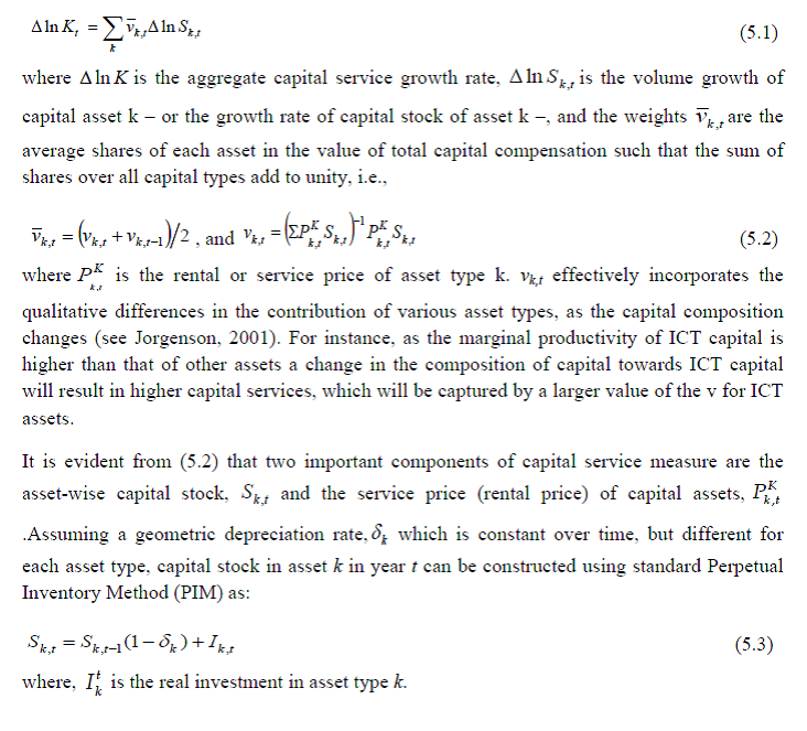 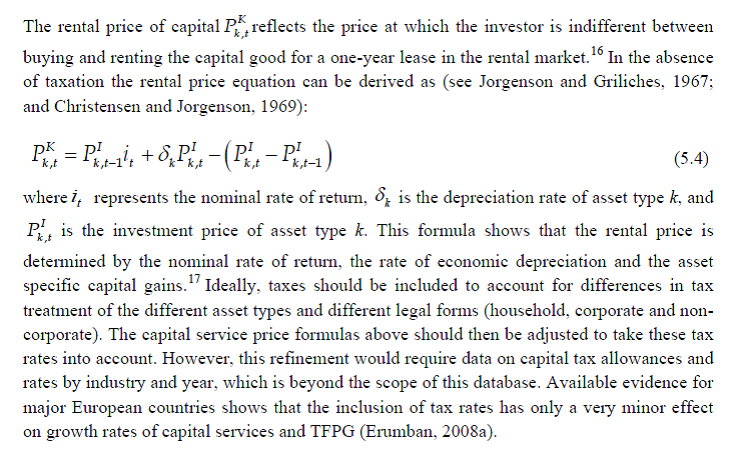 Since our measure of capital input takes account of asset heterogeneity, it was essential to obtain investment data by asset type. We distinguish between 3 different asset types – construction, transport equipment, machinery (includes ICT and non-ICT machinery).18 We exploit multiple sources of information for the construction of our database on capital services. This includes the National Accounts Statistics (NAS) that provide information on broad sectors of the economy, the Annual Survey of Industries (ASI) covering the organised manufacturing sector, the National Sample Survey Organizations (NSSO) rounds for unorganised manufacturing and Input-Output transaction tables. Even though we use multiple sources of data, our final estimates are fully consistent with the aggregate data obtained from the NAS. In addition, our approach to capital measurement is consistent with international practices such as the EU KLEMS19, which ensures the possibility of international comparisons. In what follows we discuss the various sources of data for asset-wise investment and the construction of the relevant variables, in detail. 5.2 Data and sources (a) Asset-wise investment for broad sectors of the economy Industry-level estimates of capital input require detailed asset-by-industry investment matrices. NAS provides information on aggregate capital formation by industry of use for 9 broad sectors, which, nevertheless, was not sufficient for our purpose. Therefore, we have collected more detailed data on assets and industries from the CSO.20 This is the data underlying the published aggregate gross fixed capital formation by the broad industry groups, separately for public and private sectors. For those sectors for which the investment matrices were not available from CSO, we gathered information from other sources (e.g. ASI for organised manufacturing and NSSO surveys for unorganised manufacturing) and benchmark it to the aggregate investment series from the National Accounts. Table 5.1 provides an overview of asset types available in NAS and their corresponding asset types used in our study. | Table 5.1: Capital Asset Types in National Accounts Statistics and Corresponding Our Study Types | | NAS Asset Types | India KLEMS Asset Types | | Public Sector | | Buildings | Construction | | Other construction | Construction | | Transport Equipment21 | Transport Equipment | | Machinery & Equipment | Machinery & Equipment | | Software (1999-00 onwards) | Machinery & Equipment** | | Private Sector | | Residential buildings | Construction | | Non-residential building | Construction | | Other construction | Construction | | Machinery & Equipment (incl. transport equipment) | Machinery & Equipment (transport equipment is excluded later*) | | Software (1999-00 onwards) | Machinery & Equipment** | Note: *Transport equipment was not separately available for private sector and therefore it was imputed and subtracted from machinery and equipment (See main text).
** Software is included in the machinery and equipment, as we are not distinguishing between ICT and non-ICT assets in this version.
Source: CSO, NAS Various Issues | Total investment in each asset category is calculated as the sum of private and public sector investment in each asset. Investment in transport equipment is not available separately for the private sector. We tried several approaches to impute the private sector transport equipment data. The first was to use the share of transport equipment in non-departmental enterprises. More specifically, we apply the non-departmental enterprise transport equipment to machinery & equipment (including transport equipment) ratio to machinery & equipment in private sector for each industry to obtain industry-wise transport equipment for the private sector. We take non-departmental enterprises only, rather than the entire public sector, as it may be more realistic as it consists of public sector companies and statutory corporations, excluding administrative sector. However, the sum of industry estimates generated by this approach was not consistent with the reported aggregate private sector transport equipment. Therefore, we take a second step here, which is to use the industry distribution from this series and apply it to the published total private sector transport equipment data. The estimated transport equipment is then subtracted from each industry’s total machinery & transport equipment data to obtain machinery in private sector as a residual. However, this approach generates many negative numbers in transport equipment in private sector, particularly in transport services. Therefore, we follow a third approach, which is what we finally use in the database. We first distribute the NAS total machinery in the private sector using the industry distribution of machinery and transport equipment. These estimates are then subtracted from each industry’s total machinery & transport equipment data to obtain the transport equipment investment in the private sector industries. (b) Asset-wise investment for non-NAS sectors NAS provides data only for 9 broad sectors, while we have 27 industries, which necessitated further splitting of some of the NAS sectors. This includes aggregate manufacturing (registered and unregistered separately) with 13 sub-sectors; other services into 4 sub-sectors; and real estate activities and business services into 2 sub-sectors. The manufacturing sector investment data was disaggregated into 13 sub-sectors at the 2-digit level of NIC 1998 using ASI and NSSO data, which will be discussed in detail subsequently. Investment series in the service sector has been split into sub-sectors using two alternative approaches–value added shares, and capital/labour ratio in the higher aggregate industry. However, the final data used are based on value added shares, as a sensitivity analysis did not show a significant difference between the two. In order to split the aggregate capital formation in organised manufacturing sector into 13 study sectors, we use the Annual Survey of Industries. However, the published data does not provide any asset-wise investment information; it consists of only the aggregate capital formation or the book value of fixed capital. Most studies in the past have measured gross investment as the difference between book value of the asset in period t and in period t-1 and add depreciation in period t to that. This approach has the deficiency of comparing two different samples reported in two different years, where the number of firms/factories might be different. In particular, while using this approach at the industry level, for detailed asset categories, it might generate massive negative investment. We follow an alternative approach, following ASI’s definition of gross fixed capital formation (GFCF). ASI defines GFCF as actual additions (newly purchased, second hand and own construction) minus deductions plus depreciation adjustment for discarded assets during the year. This approach is based on a single year’s sample and helps to avoid potential huge negative investment series and is also consistent with the published ASI GFCF series. The yearly detailed volumes beginning 1964-65 were used to derive the gross fixed capital formation by asset type directly. For the years 1964-1978, the relevant data are obtained from published detailed volumes. For the period, 1983-84 to 2004-05 ASI has generated detailed tables from Block C of ASI schedule that contain data on fixed assets. Data for missing years are interpolated using the changes in investment using book value method. Table 5.2 provides an overview of the asset categories available in ASI, and the relevant asset categories in our study to which they are attributed. Though ASI provides investment in land, for reasons of NAS consistency we exclude it from our database. Once the investment in each of these assets and industries are generated using ASI data, we apply this industry-asset distribution to the published aggregate NAS GFCF series for the organised manufacturing sector. It may also be noted that from 1960-61 to 1971-72, ASI data are for the census sector and from 1973-74 onwards they are for the factory sector. In order to make these two series comparable over years, we convert the data prior to 1972 to factory sector using the factory/census ratio in 1973. Thus, after these adjustments, we obtain investment data for 13 manufacturing sectors, by asset types, consistent with the NAS aggregates. | Table 5.2: Asset Types in ASI and India KLEMS | | ASI Asset Types | India KLEMS Asset Types | | Land | Excluded | | Buildings | Buildings and Construction | | Plants & Machinery | Machinery & Equipment | | Transport Equipment | Transport Equipment | | Computer Equipment including Software (from 1998) | Machinery & Equipment* | | Pollution control equipment (from 2000) | Machinery & Equipment | Note: * Computer equipment and software are included in the machinery and equipment, as we are not distinguishing between ICT and non-ICT assets in this version.
Source: CSO, NAS Various Issues | The data required for creating the gross investment series for the 13 sectors of the unorganised manufacturing sector are obtained from various rounds of NSSO surveys on unorganised manufacturing. We use 4 rounds of NSSO surveys that cover the period 1989-2006. These are 45th round (1989-90), 51st round (1994-94) 56th round (2000-01) and 62nd round (2005-06). Unit level data has been aggregated to 13 industries using the appropriate concordance tables. NSSO provides net addition to owned assets during the reference year within the block of fixed assets, and we use this as a measure of our investment. Asset classification in NSSO has changed over various rounds, and therefore, we have tried to match these with our classification as shown in Table 5.3. The investment series arrived at for four rounds were interpolated to obtain the annual time series of unorganised gross fixed capital formation by asset type. As in the case of registered sector, once the investment by asset types across industries are constructed, the asset-industry distribution is applied to the published NAS aggregate GFCF in unregistered manufacturing to obtain NAS consistent GFCF by asset type and industries. | Table 5.3: Asset Categories in NSSO Rounds | 45th Round
(1989-90) | NSSO Sectors | India KLEMS Asset Types | 51st Round
(1994-95) | 56th Round
(2000-01) | 62nd Round
(2005-06) | | Land | Land | | | Excluded | | Building | | | Construction | | | Land & Buildings | Land & Buildings | Construction (land is excluded) | | Other construction | | | Construction | | Building & other construction | | | | Construction | | Plant & machinery | Plant & machinery | Plant & machinery | Plant & machinery | Machinery & Equipment | | Transport Equipment | Transport Equipments | Transport equipment | Transport equipment | Transport Equipment | | Tools | | | Machinery & Equipment | | Other fixed assets | | | Machinery & Equipment | | Tools & other fixed assets | | Tools & other fixed assets | Tools & other fixed assets | Machinery & Equipment | | | | Software & hardware | Machinery & Equipment* | Note: For 56th and 62nd rounds, land is separated from land & buildings using land/land & building ratio from 51st round.
* Computer equipment and software are included in the machinery and equipment, as we are not distinguishing between ICT and non-ICT assets in this version.
Source: NSSO Rounds | (c) Investment Prices by Asset Types In order to compute asset-wise capital stock using PIM (equation 5.3) and rental price (equation 5.4), we require asset-wise investment price deflators. Since CSO has provided us with investment data by industries and assets both in current and constant prices, we could derive the price deflators with base 2004-2005. These deflators are directly used for all the three asset categories we have. (d) Initial Stock, Depreciation Rates and Rate of Return As is evident from equations 5.1 to 5.4, our estimates of capital input require time-series data on asset-wise capital stock. Capital stock has been constructed using perpetual inventory method (PIM), where the capital stock (S) is defined as a weighted sum of past investments with weights given by the relative efficiencies of capital goods at different ages, which requires data on current investment by asset types, investment prices by asset types and depreciation rate. Also, for the practical implementation of PIM to estimate asset-wise capital stock, we require an estimate of initial benchmark stock (see Erumban, 2008b for an in-depth discussion on this issue). NAS provides estimates of net capital stock since 1950 for all the broad sectors in its Statement 17: Net Fixed Capital Stock by industry of use. We take the NAS estimate of real net capital stock in 1950 (in 1999-2000 prices) as our benchmark stock for all non-manufacturing sectors, and for manufacturing sectors the same is taken for the year 1964.22 However, since the NAS estimate is available only for broad sectors and for aggregate capital, we use our industry-asset distribution of GFCF in order to create net fixed capital stock estimates by asset type for all the 27 industries. NAS also provides detailed tables on assumed life of assets used for computing capital stock, for private units, administrative units as well as departmental and non-departmental units by asset types.23 We use these estimates of lifetime to derive appropriate depreciation rates for non-ICT assets, using a double declining balance rate. We assume 80 years of lifetime for buildings, 20 years for transport equipment, and 25 years for machinery and equipment. The final depreciation rates used in the study are given in Table 5.4 by asset type. Subsequently, we build our capital stock series by asset types for all the 27 industries using our GFCF series from 1950 (1964) onwards for the non-manufacturing (manufacturing) sectors. | Table 5.4: Depreciation Rate by Asset Type Used in the Computation of Capital Input | | Asset Type | Depreciation Rate (per cent) | | Building and Construction | 2.5 | | Transport Equipment | 10.0 | | Machinery | 8.0 | | Note: Depreciation rates are derived using NAS life times for each asset assuming a double declining balance rate. | Our measure of capital input is arrived using equation (5.1), for which we also require estimates of rental prices (see equation 5.4). Assuming that the flow of capital services is proportional to the capital stock at the individual asset level, aggregate capital flows can be obtained using a translog quantity index by weighting growth in the stock of each asset by the average shares of each asset in the value of capital compensation, as in (5.1). The rate of return (i) in equation (5.4) represents the opportunity cost of capital and can be measured either as internal (or ex-post) rate of return or as an external (ex ante) rate of return.24 This issue will be addressed in the further revisions of the data. The present version of the database uses an external rate of return, proxied by average of return on government securities and prime lending rate obtained from the Reserve Bank of India25. Therefore, we use a real rate, which is net of capital gain. Hence, the capital gain component in equation (5.4) is excluded while estimating rental price using external rate of return, obtaining 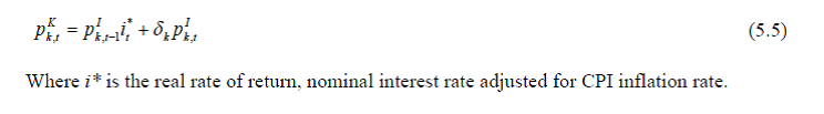 Chapter 6: Intermediate Input Series at the Industry Level In this section, we describe the basic approach we have used to derive the volume series of Intermediate Inputs namely – Energy input (E), Material input (M) and Services input (S). This breakdown of intermediate inputs can be used for extending the growth accounting exercises, but also convey interesting information about changing pattern in intermediate consumption (see e.g. JHS 2005, Chapter 4) 6.1 Methodology The methodology for measuring industry output, intermediate inputs and value added was developed by Jorgenson, Gallop and Fraumeni (1987) and extended by Jorgenson (1990 a). The cornerstone of this approach is a time series of input-output (IO) tables, which gives the flows of all commodities in the economy, as well as payments to primary factors. Every commodity is accounted for, whether produced by a domestic source or imported, and every use is noted, whether purchased by an industry or by a final demand element. All payments to factors of production i.e., labour and capital are accounted for so that all income elements of GDP are included. The methodology of constructing time series on energy, material and services inputs for the European economy has been elucidated in Timmer et al. (2010, Chapter 3). Following a similar approach as explained in Jorgenson et al. (2005, Chapter 4) and Timmer et al. (2010, Chapter 3), the time series on intermediate inputs for the India KLEMS project have been constructed. Definition of EMS: As in EU KLEMS, this study identifies three main categories of intermediate inputs. They are classified as follows: - Energy Input
- Material Input
- Service Input
Intermediate inputs are broken down into energy, material and services, based on input-output transaction tables using a standard NIC product classification. The following five energy types (and products) have been classified as the Energy input. - Coal and Lignite
- Petroleum products
- Electricity; for electricity used in the electricity sector, since there is a good amount of inter-firm sale and purchase of electricity, it has been treated as material rather than as energy
- Natural gas
- Gas (LPG)
The following fourteen input items have been classified as the Service input - Water supply
- Railway transport services
- Other transport services
- Storage and warehousing
- Communication
- Trade
- Hotels and restaurants
- Banking
- Insurance
- Ownership of dwellings
- Education and research
- Medical and health
- Other services
- Public administration
All other intermediate inputs barring the above-mentioned nineteen inputs are classified as material input. The key building block for constructing Time Series on intermediate inputs at current prices, as explained in Jorgenson et al. (2005, Chapter 4), is the input-output transaction tables, that is, the inter-industry transaction tables that provide a description of which industries produce each product and which industries use them. The IOTT gives the inter-industry transactions in value terms at factor cost presented in the form of commodity x industry matrix where the columns represent the industries and the rows as group of commodities, which are the principal products of the corresponding industries. Each row of the matrix shows in the relevant columns, the deliveries of the total output of the commodities to the different industries for intermediate consumption and final use. The entries read down industry columns give the commodity inputs of raw-materials and services, which are used to produce outputs of particular industries. The column entries at the bottom of the table give net indirect taxes (NIT) (indirect taxes – subsidies) on the inputs and the primary inputs (income from use of labour and capital), i.e., Gross Value Added (GVA). As the IOTT is in the form of commodity x industry matrix, the row totals do not tally with the column totals. The difference between each column and the corresponding row totals is due to the inclusion of the secondary products, which appear particularly in the case of manufacturing industries. This is so because by-products are also manufactured by industries in addition to their main products. Thus, while determining the entries in the rows, a by-product of an industry is transferred to the sector (commodity row), whose principal product is the same as the by-product under reference. The columns, however, show the total of principal products and by-products of each industry. All the entries in the IOTT are at factor cost, i.e. excluding trade and transport charges and NIT. The Input Flow Matrix at factor cost, published by CSO, for 1978 is a 60 x 60 matrix. The absorption matrices for 1983, 1989, 1993 and 1998 have 115 sectors. However, a detailed 130 sector absorption (commodity x industry) matrix for the Indian economy has been published from 2003-04 onwards. The scheme of sector classification adopted in IOTT 2007-08 and IOTT 2003-04 viz., IOTT 1983-84, IOTT 1989-90, IOTT 1993-94 and 1998-99 has undergone significant change with the disaggregation of some of the sectors, which have become significant in the early 2000s. -
In the agriculture and allied activities, four sectors, namely, ‘oilseeds’, ‘fruits’, ‘vegetables’ and ‘poultry & eggs’ have been introduced as separate sectors. -
In the mining sector, the sector ‘‘crude petroleum, natural gas’’ has been disaggregated into two separate sectors as ‘natural gas’ and crude petroleum’. -
The sector “Office Computing Machines” in the earlier IOTT has been eliminated due to its redundancy in the present structure of the economy. -
The sector “Miscellaneous Manufacturing” in the earlier IOTT has been disaggregated into ‘medical, precision & optical instruments’, ‘gems & jewellery’, ‘aircraft & spacecraft’ and ‘miscellaneous manufacturing’. -
“Other Transport Services” in the earlier IOTTs are further disaggregated into ‘land transport including via pipelines’, ‘water transport’, ‘air transport’ and ‘supporting and auxiliary transport activities’. -
‘‘Gas” has been regrouped in the present IOTT by merging its Gobar Gas component in the ‘other livestock product’ and LPG component in ‘petroleum products’. -
“Other Services” sector has been reorganised into separate sectors as ‘business services’, ‘computer related services’, ‘legal services’, ‘real estate service activities’, ‘renting of machinery & equipment’, ‘other community, social & personal services’ and ‘other services’. 6.2 Implementation Issues The methodology for computation of intermediate input series for 27 Industries from 1980-2011 at current and constant prices is explained in steps. Step 1: Concordance is done between IOTT and study industries -
The 60/115/130 IOTT industries are aggregated to form industries. -
A concordance table between the classification used in our study and the Input-Output Transaction Table (1998 and 2003) has been prepared. This has been attached at the end (Refer Appendix Table D). Step 2: Obtaining estimates for Material, Energy and Service Inputs for 27 Industries, in benchmark years In IOTT, no intermediate input is being used in industry 24 – ‘Public Administration’. Consequently, the intermediate input series is being estimated for only 27 industries from 1980 to 2011. The 60/115/130 commodity inputs going into the production process of output for 27 industries are aggregated into - Value of Energy Inputs used
- Value of Material Inputs used
- Value of Service Input used
- Value of Total Intermediate Inputs (summation of the above three)
Thus, for each of the benchmark years, estimates are obtained for Material, Energy and Service Inputs that has been used to produce Gross output in the 27 different India KLEMS Industries. Step 3: Projecting a time series (1980 to 2011) of proportions of Material, Energy and Service Inputs in Total Intermediate Inputs for each of the 27 industries -
For the Benchmark years i.e., 1983, 1989, 1993, 1998, 2003 and 2007, proportions of Material Inputs, Energy Inputs, and Service Inputs in Total Intermediate Inputs are calculated. -
Similar proportion for intervening years is obtained by linear interpolation of the benchmark proportions. -
This gives a time series of proportions of Material, Energy and Service Inputs in Total Intermediate Inputs for each year, from 1980 to 2011. -
Thus using IOTT, the intermediate input vector has been projected for 27 study industries from 1980 to 2011 Step 4: Consistency with NAS The projection of intermediate input vector, using IOTT in Step 3 needs to be consistent with the estimated output from NAS. -
The Gross Value of Output and the Gross Value Added at current prices calculated from NAS is taken. The difference between GVO and GVA provides us the gap between value added and gross output for each year or in other words this reflects the total intermediate inputs from NAS (GVO-GVA) -
The intermediate input vector that has been projected using IOTT in step 3 will not tally with the above estimates of total intermediate inputs from NAS. Thus the projected input vector has been proportionately adjusted to match the gap between value added and gross output obtained from NAS. This involves two steps: 1. For Benchmark years: Ratio of total intermediate inputs from NAS to that from IOTT is adjusted proportionately to the absolute value of Energy /Material /Service Inputs obtained from IOTT. 2. For Intervening Years: The interpolated proportions of energy, material and services inputs obtained from IOTT, are applied directly to the total intermediate inputs from NAS to get share of each inputs. Two examples have been given below for the construction sector: | Adjustment A: For IOTT Benchmark Year 1998 | | Source | Output/Input | Values (in ₹ crore) | | | National Account Statistics | GVO | 241873 | | | GVA | 88784 | | Total Input from NAS (GAP) | 153089 | | For Benchmark IOTT year: Absolute value of Inputs from Input-Output Transaction Table are available | Material | 73132 | | Energy | 4308 | | Service | 37399 | | Total Input from IOTT | 114839 | | Ratio of Total Input from NAS to Total Input from IOTT | Total Input from NAS/ Total Input from IOTT = 1.33 | | Adjusted Input reported | Material | = 1.33 x 73132 | 97490 | | Energy | = 1.33 x 4308 | 5743 | | Service | = 1.33 x 37399 | 49855 | | Total Input | = 1.33 x 114839 | 153089 |
| Adjustment B: For Non-Benchmark Year 1999 | | Source | Output/Input | Values (in ₹ crore) | | | National Account Statistics | GVO | 279464 | | | GVA | 102007 | | Gap | 177457 | | For Non-Benchmark IOTT year: Interpolated Proportions of Inputs from Input-Output Transaction Table have been used | Material | 0.64 | | Energy | 0.04 | | Service | 0.32 | | Total Input | 1 | | Adjusted Input reported | Material | = .64 x 177457 | 113081 | | Energy | = .04 x 177457 | 7300 | | Service | = .32 x 177457 | 57076 | | Total Input | = 1 x 177457 | 177457 | In the examples above, we can see that the total value of intermediate input exactly matches the gap between the gross value of output and gross value added. Similar adjustments have been made to construct the input series for all the other 27 study industries from 1980-2011. For every benchmark year where IOTT is available, adjustment ‘A’ has been done. For every non-benchmark year, where IOTT is not available and an intermediate input vector has been projected, adjustment ‘B’ has been done to generate the comprehensive time series of intermediate inputs consistent with the official National Accounts. Steps 1-4: This gives a Time Series of Material, Energy and Service Inputs for 27 Study Industries from 1980 to 2011 at current prices. Steps 5 and 6 below, explain the methodology for computation of intermediate input series for 27 study Industries from 1980-2011 at constant price. The approach followed here is to first form the aggregates of materials, energy and services at current price for each study industry from the benchmark Input-Output tables and then develop deflators of materials, energy and service inputs for each of the 27 study industries separately. Step 5: Constructing Deflators of Materials, Energy and Service Inputs for 27 Study Industries separately -
Deflators are obtained for each of the 115 commodity inputs (each row of the IO Matrix) -
WPI for the period 1980 to 2011 is taken from Office of the Economic Adviser, Ministry of Commerce and Industry. -
Best available Wholesale Price Index is applied to each commodity input in the IOTT. -
In several cases, no proper WPI is available for the sector; hence the best among the available has been chosen. -
In some cases, the right index has been formed from item level indices. -
In some case, one index has been removed from a higher level aggregate to generate the right index. -
For electricity as an input entering into the production process of an industry, depending on the nature of economic activity, the right price of electricity has been chosen. -
For service inputs, since WPI is not available hence implicit GDP deflators from NAS are used. -
Deflators obtained for different IO sectors have been combined using weights. The weights are based on the column of the relevant study industry in the IO table. This is because; the entries read down industry columns give the commodity inputs of raw-materials and services, which are used to produce outputs of particular industries. We have allowed for changing weights over time i.e., we have used different weights for different time periods. Two IOTT has been used for this purpose - 1989 and 2003. The price series based on the 1989 table has been used from 1980 to 1993 and the 2003 table has been used for the price series for the period 1993 to 2011. Once the two series have been formed, these have been spliced. Thus, the IO tables have been used for obtaining the materials, energy and services series for each industry at current prices. Step 6: Computing Time Series on Intermediate Input for 27 study Industries from 1980-2011, Constant prices - The deflators for material, energy and service inputs for each study industry have been used to deflate the current price intermediate input series to constant price.
Thus, we have a time series of material, energy and service inputs for 27 study Industries at constant prices. Aggregation: The report identifies six broad sectors of Total Economy. They are Agriculture; Mining and Quarrying; Manufacturing; Electricity, Gas and Water Supply; Construction and Services. For aggregation of industries, we use Tornqvist quantity index, which is a discrete time approximation to a Divisia index. This aggregation uses annual moving weights based on averages of adjacent points in time. The advantage of Tornqvist index is two-fold. First, it belongs to the preferred class of superlative indices (Diewert 1976). It exactly replicates a translog model which is flexible, that is, a model where aggregate is a linear and quadratic function of the components and time. Secondly, Tornqvist index is relatively easy to implement. 6.3 Outstanding Issues Firstly, Input-Output transaction tables are generally available on a five year interval period and this necessitates interpolation and assumption of constant shares in some cases to construct the entire time series of EMS from 1980 to 2011. Secondly, unlike studies using detailed survey data, we have to assume that all buyers pay the same price for each commodity because there is no information about price divergences. Thirdly, the estimated time series of intermediate inputs at constant prices will not be consistent with the intermediate input of NAS at constant price i.e., the deflated value of intermediate input cannot match the gap between value added and gross output at constant price from NAS. This is because NAS uses a single deflation method to estimate Gross Value Added and Gross Value of Output at constant prices. ‘However, only for one sector – Agriculture, the Gross Output and Gross Value Added, estimated by NAS is double deflated. Therefore, only for the Agriculture sector, the deflated value of intermediate input will exactly match the gap between value added and gross output at constant prices. Fourthly, there has been some confusion in the literature on the price concept to be used for intermediate inputs. It is generally acknowledged that the intermediate input weights should be measured from the user’s point of view, i.e., reflect the marginal cost paid by the user. Most studies maintain that purchaser’s price should be used. These prices include net taxes on commodities paid by the user and include margins on trade and transportation (see, for example, OECD 2001). However, when trade and transportation services are included as separate intermediate inputs, margins paid on other products should also be allocated to these services. Ideally, a distinction should be made between the intermediate product valued at purchaser’s price minus margins and the trade and transportation services valued at margins. This is the approach taken in Jorgenson, Gollop and Fraumeni (1987) and in Jorgenson et al. (2005). However, Timmer et al. (2010, Chapter 3) explains that for the EU KLEMS database, intermediate inputs have been valued at purchaser’s price owing to unavailability of necessary data. Because of the use of purchaser’s price concept the shares of services in intermediate inputs do not include trade and transportation margins. Similarly, in practice for the database, the time series of Intermediate Input constructed is at purchaser’s price i.e. it implicitly takes into account the net indirect taxes. The distribution of this net indirect tax between material, energy and services has not been possible because of unavailability of a time series of tax matrix from 1980 to 2011. | Appendix D: Concordance of Study Industries and IOTT Industries | | KLEMS Industry No. | Industry Description | Sector No. IOTT 2003 | Sector description | Sector No. IOTT 1998 | Sector description | | 1 | Agriculture, Hunting, Forestry and Fishing | 1 | Paddy | 1 | Paddy | | | | 2 | Wheat | 2 | Wheat | | | | 3 | Jowar | 3 | Jowar | | | | 4 | Bajra | 4 | Bajra | | | | 5 | Maize | 5 | Maize | | | | 6 | Gram | 6 | Gram | | | | 7 | Pulses | 7 | Pulses | | | | 8 | Sugarcane | 8 | Sugarcane | | | | 9 | Groundnut | 9 | Groundnut | | | | 10 | Jute | 10 | Jute | | | | 11 | Other Oil Seed | 11 | Cotton | | | | 12 | Cotton | 12 | Tea | | | | 13 | Tea | 13 | Coffee | | | | 14 | Coffee | 14 | Rubber | | | | 15 | Rubber | 15 | Coconut | | | | 16 | Coconut | 16 | Tobacco | | | | 17 | Tobacco | 17 | Other crops | | | | 18 | Fruits | | | | | | 19 | Vegetables | | | | | | 20 | Other crops | | | | | | 21 | Milk and milk products | 18 | Milk and milk products | | | | 22 | Animal services (agricultural) | 19 | Animal services (agricultural) | | | | 23 | Poultry & eggs | | | | | | 24 | Other livestock products | 20 | Other livestock products | | | | 25 | Forestry and logging | 21 | Forestry and logging | | | | 26 | Fishing | 22 | Fishing | | 2 | Mining & Quarrying | 27 | Coal and lignite | 23 | Coal and lignite | | | | 28 | natural gas | 24 | Crude petroleum, natural gas | | | | 29 | Crude petroleum | | | | | | 30 | Iron ore | 25 | Iron ore | | | | 31 | Manganese ore | 26 | Manganese ore | | | | 32 | Bauxite | 27 | Bauxite | | | | 33 | Copper ore | 28 | Copper ore | | | | 34 | Other metallic minerals | 29 | Other metallic minerals | | | | 35 | Lime stone | 30 | Lime stone | | | | 36 | Mica | H | Mica | | | | 37 | Other non-metallic minerals | 32 | Other non-metallic minerals | | 3 | Food Products, Beverages & Tobacco | 38 | Sugar | 33 | Sugar | | | | 39 | Khandsari, boora | 34 | Khandsari, boora | | | | 40 | Hydrogenated oil (vanaspati) | 35 | Hydrogenated oil (vanaspati) | | | | 41 | Edible oils other than vanaspati | 36 | Edible oils other than vanaspati | | | | 42 | Tea and coffee processing | 37 | Tea and coffee processing | | | | 43 | Miscellaneous food products | 38 | Miscellaneous food products | | | | 44 | Beverages | 39 | Beverages | | | | 45 | Tobacco products | 40 | Tobacco products | | 4 | Textiles, Textile Products, Leather and Footwear | 46 | Khadi, cotton textiles (handlooms) | 41 | Khadi, cotton textiles (handlooms) | | | | 47 | Cotton textiles | 42 | Cotton textiles | | | | 48 | Woolen textiles | 43 | Woolen textiles | | | | 49 | Silk textiles | 44 | Silk textiles | | | | 50 | Art silk, synthetic fiber textiles | 45 | Art silk, synthetic fiber textiles | | | | 51 | Jute, hemp, mesta textiles | 46 | Jute, hemp, mesta textiles | | | | 52 | Carpet weaving | 47 | Carpet weaving | | | | 53 | Readymade garments | 48 | Readymade garments | | | | 54 | Miscellaneous textile products | 49 | Miscellaneous textile products | | | | 59 | Leather footwear | 54 | Leather footwear | | | | 60 | Leather and leather products | 55 | Leather and leather products | | 5 | Wood and Products of Wood | 56 | Wood and wood products | 51 | Wood and wood products | | 6 | Pulp, Paper, Paper Products, Printing and Publishing | 57 | Paper, paper prods. & newsprint | 52 | Paper, paper prods. & newsprint | | | | 58 | Printing and publishing | 53 | Printing and publishing | | 7 | Coke, Refined Petroleum Products and Nuclear Fuel | 63 | Petroleum products | 58 | Petroleum products | | | | 64 | Coal tar products | 59 | Coal tar products | | 8 | Chemicals and Chemical Products | 65 | Inorganic heavy chemicals | 60 | Inorganic heavy chemicals | | | | 66 | Organic heavy chemicals | 61 | Organic heavy chemicals | | | | 67 | Fertilizers | 62 | Fertilizers | | | | 68 | Pesticides | 63 | Pesticides | | | | 69 | Paints, varnishes and lacquers | 64 | Paints, varnishes and lacquers | | | | 70 | Drugs and medicines | 65 | Drugs and medicines | | | | 71 | Soaps, cosmetics & glycerin | 66 | Soaps, cosmetics & glycerin | | | | 72 | Synthetic fibers, resin | 67 | Synthetic fibers, resin | | | | 73 | Other chemicals | 68 | Other chemicals | | 9 | Rubber and Plastic Products | 61 | Rubber products | 56 | Rubber products | | | | 62 | Plastic products | 57 | Plastic products | | 10 | Other Non-Metallic Mineral Products | 74 | Structural clay products | 69 | Structural clay products | | | | 75 | Cement | 70 | Cement | | | | 76 | Other non-metallic mineral prods. | 71 | Other non-metallic mineral prods. | | 11 | Basic Metals and Fabricated Metal Products | 77 | Iron, steel and ferro alloys | 72 | Iron, steel and ferro alloys | | | | 78 | Iron and steel casting & forging | 73 | Iron and steel casting & forging | | | | 79 | Iron and steel foundries | 74 | Iron and steel foundries | | | | 80 | Non-ferrous basic metals | 75 | Non-ferrous basic metals | | | | 81 | Hand tools, hardware | 76 | Hand tools, hardware | | | | 82 | Miscellaneous metal products | 77 | Miscellaneous metal products | | 12 | Machinery, n.e.c. | 83 | Tractors and agri. implements | 78 | Tractors and agri. implements | | | | 84 | Industrial machinery (F & T) | 79 | Industrial machinery (F & T) | | | | 85 | Industrial machinery (others) | 80 | Industrial machinery (others) | | | | 86 | Machine tools | 81 | Machine tools | | | | 87 | Other non-electrical machinery | 82 | Office computing machines | | | | | | 83 | Other non-electrical machinery | | 13 | Electrical and Optical Equipment | 88 | Electrical industrial Machinery | 84 | Electrical industrial Machinery | | | | 89 | Electrical wires & cables | 85 | Electrical wires & cables | | | | 90 | Batteries | 86 | Batteries | | | | 91 | Electrical appliances | 87 | Electrical appliances | | | | 92 | Communication equipments | 88 | Communication equipments | | | | 93 | Other electrical Machinery | 89 | Other electrical Machinery | | | | 94 | Electronic equipments (incl.TV) | 90 | Electronic equipments (incl.TV) | | | | 101 | Watches and clocks | 97 | Watches and clocks | | | | 102 | medical, precision and optical instruments | | | | 14 | Transport Equipment | 95 | Ships and boats | 91 | Ships and boats | | | | 96 | Rail equipments | 92 | Rail equipments | | | | 97 | Motor vehicles | 93 | Motor vehicles | | | | 98 | Motor cycles and scooters | 94 | Motor cycles and scooters | | | | 99 | Bicycles, cycle-rickshaw | 95 | Bicycles, cycle-rickshaw | | | | 100 | Other transport equipments | 96 | Other transport equipments | | | | 104 | Aircraft & spacecraft | | | | 15 | Manufacturing, n.e.c.; recycling | 55 | Furniture and fixtures-wooden | 50 | Furniture and fixtures-wooden | | | | 103 | gems & jewellery | | | | | | 105 | Miscellaneous manufacturing | 98 | Miscellaneous manufacturing | | 16 | Electricity, Gas and Water Supply | 107 | Electricity | 100 | Electricity | | | | 108 | Water supply | 101 | Gas | | | | | | 102 | Water supply | | 17 | Construction | 106 | Construction | 99 | Construction | | 18 | Trade | 116 | Trade | 107 | Trade | | 19 | Hotels and Restaurants | 117 | Hotels and restaurants | 108 | Hotels and restaurants | | 20 | Transport and Storage | 109 | Railway transport services | 103 | Railway transport services | | | | 110 | Land transport including via pipeline | 104 | Other transport services | | | | 111 | Water Transport | 105 | Storage and warehousing | | | | 112 | Air Transport | | | | | | 113 | Supporting and Auxiliary Transport Activities | | | | | | 114 | Storage and warehousing | | | | 21 | Post and Telecommunication | 115 | Communication | 106 | Communication | | 22 | Financial Services | 118 | Banking | 109 | Banking | | | | 119 | Insurance | 110 | Insurance | | 23 | Public Administration and Defence | 130 | Public administration | 115 | Public administration | | 24 | Education | 121 | Education and research | 112 | Education and research | | 25 | Health and Social Work | 122 | Medical and health | 113 | Medical and health | | 26 | Other Services | 120 | Ownership of dwellings | 111 | Ownership of dwellings | | | | 123 | Business services | 114 | Other services | | | | 124 | Computer and related activities | | | | | | 125 | Legal services | | | | | | 126 | Real estate activities | | | | | | 127 | Renting of machinery and equipment | | | | | | 128 | Other communication, social and personal services | | | | | | 129 | Other services | | | | Source: Input-Output Transaction Table 1998, 2003. | Chapter 7: Factor Income Share Series at the Industry Level The distribution of income between capital, labour and intermediate inputs, is an important element in growth accounting because income shares, under conditions of competitive markets, can be used to measure the contributions each factor makes towards output growth. 7.1 Methodology for Measuring Labour Income Share Series Under the assumption of constant returns to scale with two factors of production i.e., labour and capital, the sum of the labour income share and capital income share is 1. The labour income share is defined as the ratio of labour income to GVA. Capital income share is accordingly obtained as one minus labour income share. There are no published data on factor income shares in Indian economy at a detailed disaggregate level. National Accounts Statistics (NAS) of the CSO publishes the Net Domestic Product (NDP) series comprising of compensation of employees (CE), operating surplus (OS) and mixed income (MI) for the NAS industries. The income of the self-employed persons, i.e. MI is not separated into the labour component and capital component of the income. Therefore, to compute the labour income share out of value added, one has to take the sum of the compensation of employees and that part of the MI which are wages for labour. The computation of labour income share for the 27 study industries involves two steps. First, estimates of CE, OS and MI have to be obtained for each of the 27 study industries from the NAS data which are available only for the NAS sectors (see Table 7.1). Second, the estimate of MI has to be split into labour income and capital income for each industry for each year (except for those industries for which the reported MI is zero, for instance, public administration). | Table 7.1: NAS Sectors and Corresponding Study Industries for Computation of Labour Income Shares | | NAS sectors for which factor income data are available | Corresponding Study Industries | | 1. Agriculture, forestry & logging and fishing | 1 | Agriculture, Hunting, Forestry and Fishing | | 2. Mining & Quarrying | 2 | Mining and Quarrying | | 3.1 Manufacturing-registered | 3 | Food Products, Beverages and Tobacco | | 3.2 Manufacturing - unregistered | 4 | Textiles, Textile Products, Leather and Footwear | | Both registered and unregistered manufacturing are split into 13 manufacturing industries (3 to 15) | 5 | Wood and Products of Wood | | | 6 | Pulp, Paper, Paper Products, Printing and Publishing | | | 7 | Coke, Refined Petroleum Products and Nuclear Fuel | | | 8 | Chemicals and Chemical Products | | | 9 | Rubber and Plastic Products | | | 10 | Other Non-Metallic Mineral Products | | | 11 | Basic Metals and Fabricated Metal Products | | | 12 | Machinery, n.e.c. | | | 13 | Electrical and Optical Equipment | | | 14 | Transport Equipment | | | 15 | Manufacturing, n.e.c.; recycling | | 4. Electricity, gas and water supply | 16 | Electricity, Gas and Water Supply | | 5. Construction | 17 | Construction | | 6.1 Trade | 18 | Trade | | 6.2 Hotels and restaurants | 19 | Hotels and Restaurants | | 7.1 Railways | 20 | Transport and Storage | | 7.2 Transport by other means | | | | 7.3 storage | | | | 7.4 Communication | 21 | Post and Telecommunication | | 8.1 Banking and Insurance | 22 | Financial Intermediation | | 9.1 Public administration and Defence | 24 | Public Administration & Defence; Compulsory Social Security | | 9.2 +8.2 Other Services plus | 25 | Education | | Real Estates, ownership of dwelling and business services | 26 | Health and Social Work | | | 23 | Business Services | | 27 | Other Services* | | Note: *Study Industry ‘Other Services’ includes Real Estate Activities; Other Community, Social and Personal Services, Private Household with Employed Persons. | Basic data sources used for the computation of labour income share are NAS, ASI and unit level data of survey of unorganised manufacturing enterprises. These data sources are used to obtain estimates of CE, OS and MI for each of the 27 study industries. For splitting the labour and non-labour components out of the MI of self-employed, the unit level data of NSS employment-unemployment surveys are used along with the estimates of CE, OS and MI basically obtained from the NAS. 7.2 Implementation Issues a) Construction of Labour Income Share Series in Gross Value Added The estimation of labour income share for the 27 study industries has been done in two steps, as discussed below. Step 1: Estimation of CE, OS and MI for the 27 study Industries For some industries under study, for instance (i) Agriculture, forestry & logging and fishing, (ii) Mining & quarrying, (iii) Electricity, gas and water supply, and (iv) Construction, the required data are readily available from NAS. For others, the estimates available in NAS have to be distributed across the study industries. In certain cases, the estimates of CE, OS and MI for a particular NAS sector have been distributed across constituent study industries proportionately in accordance with the gross value added in those industries. Estimate of factor incomes for ‘other services’ in NAS, for instance, has been split into estimates for (i) Education, (ii) Health and Social Work, and (iii) Other Community, Social and Personal Services including Renting of machinery and business services, and Private Household with Employed Persons. NAS provides estimates of factor incomes for registered manufacturing and unregistered manufacturing, but not for individual manufacturing industries. The NAS estimates of factor incomes for registered manufacturing have to be split into various manufacturing industries considered in the study (13 in number) using ASI data. The reported CE in NAS for registered manufacturing has been distributed into those 13 industries in proportion to the reported ASI data on emoluments for various industries. In a similar way, using ASI data, the estimate of OS for registered manufacturing has been distributed. Emoluments are subtracted from gross value added for various industries yielding capital income. The share of different industries in aggregate capital income of organised manufacturing indicated by the ASI data is used to split the estimate of OS for registered manufacturing reported in the NAS. The methodology applied for unregistered manufacturing is similar. The published results and unit level data of survey of unorganised manufacturing industries have been used for this purpose. The estimates of wage payments (to hired workers) in different industries have been used to split (proportionately) the estimate of CE in the NAS for aggregate unregistered manufacturing. The estimated wage payment is subtracted from the estimated value added to obtain an estimate of capital income and mixed income of the self-employed in various unorganised manufacturing industries. The estimate of MI provided in NAS for unregistered manufacturing has then been proportionately distributed across industries using the estimate of capital income and mixed income of the self-employed in various industries that could be formed on the basis of published results and unit level data of survey of unorganised manufacturing industries. Unlike the ASI data for organised manufacturing, the data for unorganised manufacturing enterprises are available for only select years. The proportions mentioned above could, therefore, be computed only for those select years (data for five rounds have been used; these are for the 45th round (1989-90), 51st round (1994-95), 56th round (2000-01), 62nd round (2005-06) and 67th round (2010-11)). It has accordingly been necessary to resort to interpolation/ extrapolation to obtain the relevant proportions for other years. Step 2: Splitting of MI into Labour Income and Capital Income As explained above, the income share of labour is computed as: The derivation of the GVA series for different industries has been briefly explained in Chapter 2. The derivation of CE and MI series has been explained in step I above. Therefore, only the estimation method of ƞ needs to be described. The estimation of ƞ has been done with the help of NSS survey-based estimates of employment of different categories of workers (number of persons and days of work) and wage rates (which has been described briefly in Chapter 4) coupled with estimates of MI, basically obtained from the NAS. Two approaches have been taken to get an estimate of ƞ, and the labour income share series for different industries finally adopted in the study makes use of an average of the estimates of ƞ obtained by the two approaches. In the first approach, an estimate of labour income of self-employed workers has been made for each study industry for five years, 1983-84, 1987-88, 1993-94, 1999-00, 2004-05, 2009-10 and 2011-12 on the basis of the estimated number of self-employed, wage rate of self-employed and the number of days of work per week. The industry-wise estimates of number of self-employed, wage rate of self-employed and the number of days of work per week has been made from unit records of NSS employment-unemployment surveys (major rounds), as explained in Chapter 4 above. The estimates of the number of self-employed, wage rate of self-employed and the number of days of work per week provide an estimate of the annual labour income of self-employed workers which is divided by the mixed income of self-employed (derived from NAS) to get an estimate of ƞ. For five industries, the ratio in question has been computed and applied. For the other 22 industries, the ratio in question has been computed after clubbing the industries into 11 industry groups.26 In the latter case, a common ratio computed for a group of industries has then been applied to constituent industries. The list of industries or industry groups for which ƞ has been estimated is given in table 7.2. In the second approach, the NSS data are used to compute the following ratio: the ratio of labour income of self-employed workers to the labour income of regular and casual workers. Let this be denoted by θ. Then, the estimate of CE provided in the NAS is multiplied by θ to obtain an estimate of the labour income component out of the MI reported in the NAS. The labour component of MI divided by total MI gives an estimate of ƞ. In case the estimated labour component of MI exceeds the estimate of MI, the estimate of ƞ has been taken as unity. Examining the estimates obtained by the first approach, it was found that the estimated labour income share out of mixed income varied significantly among the estimates for the seven years for which the ratio in question has been estimated. The estimates of ƞ obtained by the second approach has the problem that in a number of cases, the estimated labour component of MI exceeds the estimate of MI given in the NAS, and therefore ƞ is taken as one. The method finally adopted is as follows: (a) The average value of ƞ has been computed for each industry or industry group by taking the estimates for the years 1983-84, 1987-88, 1993-94, 1999-00, 2004-05, 2009-10 and 2011-12. This has been done separately for the estimates based on approach-1 and those based on approach-2. (b) The estimates of ƞ obtained for each industry or industry group by the two approaches have then been averaged. (c) Having obtained an estimate of ƞ, equation 6.1 given above has been applied to compute the labour income share. | Table 7.2: Industries and Groups for which ƞ (proportion of labour income out of mixed income) has been estimated | | Industry/ Industry Group | Study Industries | | Agriculture, Hunting, Forestry and Fishing | Agriculture, Hunting, Forestry and Fishing | | Mining and Quarrying | Mining and Quarrying | | Food products, beverages, tobacco, textiles, leather products | Food Products, Beverages and Tobacco | | | Textiles, Textile Products, Leather and Footwear | | Wood, wood products, paper and printing | Wood and Products of Wood | | | Pulp, Paper, Paper Products, Printing and Publishing | | Petroleum products, chemical products, rubber and plastic products | Coke, Refined Petroleum Products and Nuclear Fuel | | | Chemicals and Chemical Products | | | Rubber and Plastic Products | | Other Non-Metallic Mineral Products | Other Non-Metallic Mineral Products | | Metals, metal products, machinery and transport equipment | Basic Metals and Fabricated Metal Products | | | Machinery, n.e.c. | | | Electrical and Optical Equipment | | | Transport Equipment | | Manufacturing, n.e.c; recycling | Manufacturing, n.e.c; recycling | | Electricity, Gas and Water Supply | Electricity, Gas and Water Supply | | Construction | Construction | | Trade, hotels, restaurants | Trade | | | Hotels and Restaurants | | Transport, storage and communication | Transport and Storage | | | Post and Telecommunication | | Public administration & defence | Public Administration and Defence; Compulsory Social Security | | Education and health | Education | | | Health and Social Work | | Other services including financial services, real estates, business services | Financial Intermediation | | Business Services | | Other Services | | Source: National Account Statistics (NAS) reports. | b) Construction of Factor Income Share Series in Gross Output The income share of labour, capital and intermediate inputs in Gross output has been computed using the following steps: -
The individual shares of intermediate inputs i.e. energy, material and services in Gross output are calculated. -
The labour income and capital income out of GVA are further distributed into income share of labour in gross output and income share of capital in gross output. -
Thus, we get the share of labour, capital, material, energy and services in output. -
For agriculture sector, land is taken as an input. First, the income share of intermediate inputs in gross output is calculated. Then the non-labour income (out of value added) in agriculture is distributed equally between land and capital inputs to derive weights. 7.3. Outstanding Issues The splitting of unorganised sector factor incomes into individual industries has been done using unorganised sector survey results. The proportions computed for 1983-84 has been applied for the period 1980-81 to 1983-84. While there were surveys of unorganised manufacturing enterprises in 1978-79 and 1984-85, the survey results have not been used for estimation of factor incomes in different industries of the unorganised manufacturing sector. An attempt will be made to use survey data for the years 1978-79 and 1984-85 rather than applying the proportions computed for 1989-90 to factor income data for earlier years. The present study provides estimates of income shares for manufacturing and its sub-branches. An attempt will be made in the third phase of the study to split manufacturing sector into organised manufacturing and unorganised manufacturing segments. The output and inputs series will be constructed separately for organised and unorganised manufacturing sectors. However, given the employment potential and sizable presence of the unorganised segment in many of the manufacturing industries, it would be worthwhile in Indian context to examine separately the productivity performances of the organised and unorganised components of Indian manufacturing. Thus, in the third phase of this project, the labour income series will have to be computed for the organised and unorganised sectors manufacturing separately. Chapter 8: Growth Accounting Methodology This chapter deals with the methodology of measurement of total factor productivity (TFP) growth for individual industries in the KLEMS framework and the aggregation from industry level productivity measures to measures for broad sectors and the economy as a whole. The methodology of analysis of sources of gross output growth at the individual industry level and sources of GVA (Gross Value Added) or GDP growth at the broad sector level and the economy level will also be presented in this chapter. 8.1 Methodology for Measuring Productivity Growth at the Industry level The production function Our measurement of TFP growth for different industries of the Indian economy is based on a gross output production function for each industry j: Y = f (L (L1,…Ln), K (K1…Km), E (E1….Es), M (M1 …Mu), S (S1 … Sv ), T) (8.1) Y is industry gross output, L is labour input, K is capital input and E, M and S are intermediate inputs-namely energy, material and services and T is an indicator of technology for industry j. All variables are indexed by time (t subscript is suppressed). There are several things to note about the production function- (1) all variables are aggregates of many components that have been discussed in the earlier report/ chapters; (2) we assume that the industry production function is separable in these aggregates; (3) time (indicator of technology) enters the production function symmetrically and directly with inputs. An important feature of the gross output approach is the explicit role of intermediate inputs. In our study, we have considered three intermediate inputs - energy, material and services and this is important as we may find that intermediate inputs are the primary component of some industries outputs.27 Failure to quantify intermediate inputs leads us to miss both the role of key industries that produce intermediate inputs and the importance of intermediate inputs for the industries that use them. In order to estimate the production function at constant prices, the industry level price data is used for output, capital, labour and intermediate inputs, e.g., PYj; PLj, PKj; PEj, PMj, PSj. We assume that all industries face the same input prices. The industry price of an input varies across industries due to compositional effects as industries expend different shares of their investment on each type of asset. The same is true for all inputs. 8.2 Methodology for Aggregation across Industries In the analysis presented in the above section, gross value of output (GVO) is taken as the measure of output of an industry and TFP growth was estimated using the gross output function framework in which capital, labour, material, energy and services are taken as five inputs (in the case of agriculture, land was included among inputs). The Tornqvist index is applied to estimate TFP growth for each year during 1980-81 to 2011-12, which yielded an index of TFP for each industry for that period, permitting estimation of trend growth rate in TFP for the period under study (1980-81 to 2011-12). The method of estimation of TFP growth for individual industries described in section 7.1 cannot be readily applied to a higher level of aggregation. The main problem is that gross value of output cannot be added across industries to generate a measure of output at a higher level of aggregation, say for the economy or of any of the broad sectors. It becomes necessary, therefore, to consider appropriate methods of aggregation across industries consistent with the gross output function specification at the individual industry level. It is needless to say that one has to use the concept of value added to define an appropriate measure of output at the economy or broad sector level, but even here there are important issues of aggregation, i.e., how value added in different industries should be combined. A very useful discussion of the issues involved is found in Jorgenson et al. (2005). There are three approaches to estimating TFP growth at an aggregate level. This is discussed in detail in Jorgenson et al. (2005). The first approach is called aggregate production function approach. This approach assumes the existence of an aggregate production function (say, at the level of the economy or at the level of manufacturing or services sector). An essential condition is that the production function be separable in primary inputs. Let the production function for a particular industry be defined as: Y =f (X, K, L, T), (8.8) where Y denotes gross output, X intermediate input (in turn a combination of material, energy and services), K capital input, L labour input and T time (representing technology). Then, the concept of value added requires the existence of a value added function which in turn requires that the above production function be separable in K, L and T, i.e., the production function should take the following form: Y =g (X, V (K, L, T)). (8.9) In this equation, V (.) is the value added function. V denotes value added. Besides the condition of separability of the production function described above, a number of highly restrictive assumptions have to be made for the aggregate production function approach. These include: (a) the value added function is the same across all industries up to a scalar multiple, (b) the functions that aggregate heterogeneous types of labour and capital must be identical in all industries, and (c) each specific type of capital and labour receives the same price in all industries. With these assumptions made, real value added at the aggregate level becomes a simple addition of real value added in individual industries. In notation, 8.3 Implementation Issues The data constructed for gross value added and gross output, labour input, capital inputs, intermediate inputs and factor income shares (Chapters 2, 3, 4, 5, 6 and 7 respectively), are used to estimate TFPG during the period 1980 to 2011. Labour input is measured using total person worked (see, Chapter 4 for the detailed discussion). The series on investment in capital services (including ICT) are taken from Chapter 5.
Bibliography Aggarwal, Suresh Chand (2004), “Labour Quality in Indian Manufacturing: A State Level Analysis”, Economic and Political Weekly, Vol. 39(50), pp.5335‐44. Bhalla, Surjit S. and Tirthatanmoy Das (2005), “Pre‐ and Post‐Reform India: A Revised Look at Employment”, Wages and Inequality, India Policy Forum, Vol. 2, NCAER, New Delhi. Bosworth B., Collins S. and Virmani A. (2007), “Sources of Growth in Indian Economy”, NBER Working Paper No. 12901. Bosworth, Barry and Susan M. Collins (2008), “Accounting for Growth: Comparing China and India”, Journal of Economic Perspectives, American Economic Association, Winter, 22(1): 45‐66. Christensen, L.R. and Jorgenson D.W. (1969), “The Measurement of US Real Capital Input, 1929‐x”, Review of Income and Wealth, 15, 293‐320. CSO (2007), “National Accounts Statistics: Sources and Methods”, available at http://mospi.nic.in/ Central Statistical Organization: Population of India, different years. Diewert, W.E. (1976), “Exact and Superlative Index Numbers”, Journal of Econometrics, 4, 115‐145. Diewert, E (1980), Aggregation Problems in the Measurement of Capital, in Usher, D (eds.), The Measurement of Capital, Chicago, The University of Chicago Press. Erumban, A, A (2008a), “Rental Prices, Rates of Return, Capital Aggregation and Productivity: Evidence from EU and US”, CESifo Economic Studies, 3 (54), 499‐533. Erumban, A, A (2008b), Measurement and Analysis of Capital, Productivity and Economic Growth, SOM theses series, University of Groningen (available http://irs.ub.rug.nl/ppn/315102683). Jorgenson, D.W and Z. Griliches (1967), “The Explanation of Productivity Change”, Review of Economic Studies, 34, 249‐283. Jorgenson, D. W. et al. (1987), Productivity and US Economic Growth, Harvard University Press, Cambridge Mass. Jorgenson, D and K Vu (2005), “Information Technology and the World Economy”, Scandinavian Journal of Economics 107(4), 631-650, 2005. Jorgenson D.W. and Stiroh K.J. (2000), “Raising the Speed Limit: U.S. Economic Growth in the Information Age”, Brookings Papers on Economic Activity, (1), 125‐211. Jorgenson, D. W., Ho, M. S. and Stiroh, K. J. (2005), “Information Technology and the American Growth Resurgence”, MIT Press, Cambridge. OECD (2001): OECD Productivity Manual, Paris. O’Mahony, M. and M.P. Timmer (2009), “Output, Input and Productivity Measures at the Industry Level: The EU India KLEMS database”, Economic Journal, 119(538), pp. F374‐ F403. Rangarajan C. (2009), India Monetary Policy, Financial Stability and Other Essays, Academic Foundation, New Delhi. Sailaja, M. (1988), Productivity in the Service Sector: The Case of Indian Railways, 1950‐ 51 to 1985‐86, unpublished Ph.D. thesis, Delhi School of Economics, Delhi. Sivasubramanian S. (2004), The Sources of Economic Growth in India: 1950‐51 to 1999‐ 2000, New Delhi: Oxford University Press. Srinivasan, T. N. (2008), “Employment and Unemployment since the Early 1970’s”, India Development Report, OUP, Mumbai. Sundaram, K. (2007), “Employment and Poverty in India, 2000‐2005”, Economic and Political Weekly, Vol. XLII (30), pp. 3121‐31. Sundaram, K (2009), “Measurement of Employment and Unemployment in India: some issues”, Working Paper No. 174, Centre for Development Economics, Department of Economics, Delhi School of Economics, Delhi. Timmer, M.P, Mahony, M. and van Ark, B. (2007), The EU KLEMS Growth and Productivity Accounts: An Overview, Mimeo University of Groningen & University of Birmingham. Timmer, Marcel P.; Robert Inklaar; Mary O’Mahony and Bart van Ark (2010), Economic Growth in Europe: A Comparative Industry Perspective, Cambridge: Cambridge University Press. Visaria, P (1996), “Structure of Indian Workforce, 1961‐1994”, Indian Journal of Labour Economics, New Delhi, pp.725‐739.
| List of Abbreviations | | ASI | Annual Survey of Industries | | CE | Compensation of Employees | | CPI | Consumer Price Index | | CSO | Central Statistics Office | | CDS | Current Daily Status | | CWS | Current Weekly Status | | EU | European Union | | EUS | Employment and Unemployment Surveys | | FISIM | Financial Intermediation Services Indirectly Measured | | GDP | Gross Domestic Product | | GFCF | Gross Fixed Capital Formation | | GVA | Gross Value Added | | GVO | Gross Value of Output | | ICT | Information and Communication Technology | | IOTT | Input-Output Transaction Table | | ISIC | International Standard Industrial Classification | | MI | Mixed Income | | NAS | National Accounts Statistics | | NIC | National Industrial Classification | | NIT | Net Indirect Tax | | NSSO | National Sample Survey Organisation | | OS | Operating Surplus | | PIM | Perpetual Inventory Method | | RBI | Reserve Bank of India | | SNA | System of National Accounts | | TFP | Total Factor Productivity | | UPS | Usual Principal Status | | UPS | Usual Principal and Subsidiary Status | | WPI | Wholesale Price Index | | WPR | Work Participation Rate |
|