Capacity utilization (CU) is an important economic indicator to assess demand and investment prospects of the economy and presumed to provide a reliable indication of incipient inflationary pressure. This article attempts to empirically investigate CU- manufacturing and price linkages by using CU estimated by the Order Books, Inventories and Capacity Utilisation Survey of the Reserve Bank and a longer time series of CU constructed using an alternate method. The findings suggest that the relationship between CU and WPI- manufacturing based inflation varies over different sample periods. The aggregate level CU needs to be interpreted prudently for gauging future path of manufacturing inflation.

Introduction

Capacity Utilisation (CU) is harnessing the installed capacity using available resources, to produce desired output during a given period. In simpler terms, CU is the ratio of actual output to the potential output that can be produced under normal conditions. The potential output capacity depends on available capital (i.e., machine/ equipment, building/ factory, etc.) and labour to produce maximum level of output on sustainable basis within the framework of a realistic work schedule, taking into account normal downtime and assuming sufficient availability of inputs to operate machinery and equipments. In any manufacturing process, installation of production capacity and its utilization depends on the business prospects, prevailing and expected demand conditions. The CU reflects demand conditions in an economy where production processes respond to changing demand and CU fluctuates accordingly. Rising demand may translate into upward pressure on the general price level and so higher CU can be accompanied by rise in inflation. However, literature is also of the view that the relationship between CU and inflation vary over time. So empirical investigation is required to understand capacity utilization relationship with prices and its predictive power for inflation.

At present, in India, there is no single official estimate of CU in the manufacturing sector. The annual accounts of companies do not report required parameters uniformly. Use of industrial production data and surveys are alternate ways to get some insights into CU rates at plant or company level and then aggregated at the industry or economy level. Surveys, that provide insights into CU, can be broadly classified into two categories; qualitative: Business Tendency/ Conditions Surveys (e.g., Industrial Outlook Survey of the Reserve Bank), and surveys which gather actual data (like, Order Books, Inventories and Capacity Utilisation Survey (OBICUS) of the Reserve Bank) on utilization of installed capacity. The OBICUS is a quarterly quantitative survey, commenced in 2008, which collects information on product-wise utilized production capacity at the firm level to derive aggregate level CU. Higher CU, accompanied by order book growth, signals robust demand conditions in the economy.

A study of country practices reveals that official estimate of CU rate is not released by many countries. However, in some countries, the compilation and dissemination of CU estimates for the manufacturing sector is undertaken either by the central bank or the government’s statistics department and estimates are mainly based on various industrial surveys (Mukherjee and Misra, 2012)¹.

Linkages between CU derived from OBICUS with output gap and investment have been explored to some extent in a few research work, while this study attempts to validate the prices and CU relationship in the context of Indian manufacturing sector. The rest of the article is organised into four sections. Section II provides literature in brief about connection between utilisation of production capacity, prices and inflation. Section III presents the stylised facts of survey-based CU rate and its long-time series computed by an alternative method. Empirical results are presented in Section IV and concluding observations are summarised in Section V.

II. Capacity Utilisation and Prices Connection: Literature Review

Keynes in his General Theory of Employment, Interest and Money postulates that the intensity with which factors of productions like capital, labour are used has an impact on cost of production and in turn, on inflation. If the economy is functioning at well below full employment level, a monetary policy induced aggregate demand shock will not result in increased wages and additional labour required by firm would be available at the current wage rate. However, when firms reach their peak level of CU, with a small increase in aggregate demand, prices may rise at a faster pace.

Persistent demand conditions may induce producers to expand their capital stock or firms may try to secure higher profit margin by raising product prices. Thus, higher level of CU can be followed by the inflationary pressure. However, the rise in price will not necessarily equal the rise in marginal cost if the firm is able to exploit market power; in that case, the markup of price over marginal cost would not have a simple relationship to current output levels. On expectations of persistent demand in future as well, firms may go for addition of production capacity and do investment and hire labour, to fulfill market demand. With the addition of capacity, the CU rate will gradually return to its ‘normal’ level, based on current production levels. Moreover, the relationship between CU and price change need not be always in positive direction. In the presence of either market power or short-run increasing returns, economic theory admits the possibility of a negative correlation between capacity utilisation and price changes (Corrado and Mattey, 1997). That means firms would maximize profit by increasing utilisation and pushing down prices.

Further, when industry has excess capacity, market competition is likely to control price rise; and in weak demand conditions, CU rate would be lower, and it may not have any impact on prices. Thus, the relationship between CU and price change may not hold constant across time and across markets. There are many other economic factors which would influence this equation such as technological progress that may have positive impact on CU and output level, rising global trade, exchange rates, inflation caused by imported goods, monetary policy stance etc., that may impact both CU and prices differently.

CU being cyclical, its relationship with prices could change depending on its position in the cycle. Business cycles are identified as having four distinct phases: trough, expansion, peak, and contraction. For a typical business cycle, potential links between four stages of CU cycle and prices are presented in the Table 1.

Generally, it is believed that increasing CU is indication of future inflationary pressure, but need not be always true. Relationship between both the indicators could vary and references about negative relationship is also found in literature. In the study of CU of the industry and CPI based annualized quarter-to-quarter inflation for the United States, Finn (1996), devised a neoclassical theory to offer an explanation of inflation and CU relationships. It states that negative co-movement of inflation and utilization occurs in response to energy price shocks. A rise in energy prices, by making energy usage more costly, reduces energy input into production. As the utlilisation of capital requires energy, utilization must decline along with energy and this output contraction induces a rise in inflation in absence of an offsetting reduction in money growth. The author further showed how shocks to production technology that are directly accommodated by money growth are an important source of positive co-movement between utilization and inflation.

Although the Keynes theory was postulated as a relationship between the price level and utilisation, the recent literature links inflation with CU. While examining the relationship between the manufacturing CU by Federal Reserve Board and core inflation (personal consumption expenditures based), Dotsey and Stark (2005) argued that this relation is not a stable one. The joint behaviour of utilization and inflation could vary over time for a number of reasons. The relationship could be sensitive to fundamental factors which are driving the economy and the way in which monetary policy responds to those fundamentals. This makes the relationship quite complex and conditional on economic circumstances. Therefore, according to the authors, drawing inferences about how capacity utilisation will affect inflation is a bit tricky and it depends on both the types of shocks hitting the economy and the central bank’s response to those shocks. This article tests the argument of non-stable relationship between CU and inflation using data specific to the Indian manufacturing sector.

III. Stylised Facts

CU estimation by survey method (OBICUS)

The OBICUS survey questionnaire is canvassed among a fixed panel of 2,500 manufacturing companies, which is common with business tendency survey. The sampling method used for the survey is purposive (non-random) and the companies have been empanelled to have a good size-mix of industries, both in public and private sector. The panel is updated periodically (with addition of new companies or deletion of closed/merged companies). However, responding to the survey is voluntary and response rate is around 45-50 per cent.

The survey questionnaire seeks data on order books (including export order), inventories (finished goods and work-in-progress), product-wise installed capacity, quantity produced in physical terms, utilization of installed capacity and actual production in value term, on a quarterly basis. The questionnaire has three blocks: block 1 is about identification details of the company; block 2 has order books and inventories information and block 3 is about collection of utilization of installed capacity details for products manufactured by companies. Currently, National Industrial Classification (NIC-2008) codes (5-digits) are being used for industry classification of manufactured products reported by companies.

The computation of CU rate at aggregate level is done with aggregation of product-wise utilization of installed capacity reported by companies from the 5-digit (NIC-2008) industry code level in first stage to the 3-digit group level. Weighted average is computed with the weights being proportional to the product’s installed capacity, in terms of reported value. Then 2 digits and final aggregate CU rate computation is done by using Gross Value Added (GVA) as weights at 3-digit and 2-digit level NIC-2008 codes respectively, weights are being taken from Annual Survey of Industries (ASI), 2013-14².

The time series of OBICUS based CU rates, since its inception in year 2008, is presented in Chart 1 along with WPI-manufacturing based (y-o-y) inflation and de-trended Index of Industrial Production (IIP)- manufacturing³. CU rates are largely able to track the manufacturing activities in the economy, as reflected in their co-movement with the de-trended IIP for manufacturing sector⁴. Since June 2013 aggregate level CU has moved in the range of 70-75 per cent, except December 2018 and March 2019 quarter wherein CU was at 76 per cent.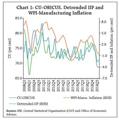

Furthermore, CU rate computed since June 2008, had contemporaneous significantly positive correlation with WPI-manufacturing based inflation at 46 per cent while the coefficient rises to 53 per cent and significant when CU rates are taken at a quarter lag. Higher rate of CU indicates strong demand in the economy and it may also be indication of likely rise in inflation in the near term. The firm level data indicates that quarterly changes in CU generally happen due to change in demand. Prices are stickier and firms may not reduce it instantly on decline in demand, they would wait to reduce prices while CU can go down more quickly. For instance, the OBICUS based CU rate during September 2018 to September 2019 declined by 5.7 percentage points from 74.8 per cent to 69.1 per cent while price level remained almost same during the period (with annual inflation of -0.06 per cent).

A longer time series of CU may help to explore this relationship further as the time series data of OBICUS may not be adequate for it. Therefore, an alternate method is used to compute the CU rates over a longer time horizon which allows studying the cyclical pattern in CU and its relation with price change.

CU estimation with an alternative method – Wharton method

As RBI’s survey-based time series of CU is available only since June-2008 quarter, and in order to study cyclical pattern of CU, a longer time series is essential, an alternative CU series is derived by applying the Wharton method. The method is chosen as it requires production data which is available easily at monthly frequency. Quarterly averages of monthly IIP-manufacturing data released by National Statistical Office are taken as actual output⁵. Peak output points in the IIP cycle, where output in a period exceeds that in the predecessor and successor period, are then identified and it is assumed that the output at these cyclical peaks indicate the capacity output i.e., the industry can produce at the time of the peak. Then CU rates are computed by expressing actual output as the percentage of estimated capacity output and the CU rate at peak points is 100 per cent.

During the intervening period i.e., between two peaks, capacity output is obtained by interpolation. Interpolation is carried out simply by joining the successive peaks by straight line. Since the actual output is below the linearly generated potential output, utilization rates between peaks are less than 100 per cent. For the periods prior to first peak and after last peak, capacity output is estimated by extrapolation and capacity output is defined as lying on the line that has the same slope as that connected the closest two peaks.

The cycle for the IIP-manufacturing reference series is extracted using the de-seasonalised and de-trended series. X-12-ARIMA technique is applied to make series seasonally adjusted then it is de-trended using HP filter (for quarterly series λ is fixed at 1600 as per the standard practice). IIP-manufacturing production data series since 1981Q2 (April-June 1981) to 2019Q4 (October-December 2019) is used to derive CU rate by using Wharton method. In the IIP cycle, turning points i.e., the peak output periods are determined by using the Bry-Boschan rule. The peak quarterly output was found in June 1988, March 1990, June 1996, June 2000, September 2004, March 2008, March 2011, September 2014, June 2016 and March 2018 (Chart 2).

Chart 3 presents the results of CU computed by Wharton method along with actual IIP and trend line drawn with help of identified peak output points.

First peak is being identified at June 1988, CU rate are computed through linear interpolation method from that point onwards while CU rates since last identified peak point i.e., March 2018 are computed through extrapolation of IIP trend line. The CU rate during June 1993 was at lowest level in the study period i.e., around 83 per cent, while global financial crisis led to another low level of CU in the series at 87.6 per cent in March 2009, after that it had moved in a narrow range. The summary statistics of CU computed by both the methods are given in Table 2. The long-term series of CU is stationary which is established by both ADF and PP test and same is confirmed for CU rate estimated by survey method by PP test. Both the CU series had positive and significant correlation of 56 per cent since June-2013 quarter.

Although the Wharton method for computation of CU is simple one, it has drawbacks too. Notably, the methodology does not distinguish changes in the intensity of utlisation of resources at different peak points, it considers utilization rate same at 100 per cent. While in reality maximum utilisation of installed production capacity could vary at peak points, also from company to company and at aggregate level for different countries too. Therefore, Wharton method provides only the CU rate relative to other periods and not the actual CU estimate. For instance, four peak points detected in the production cycle during OBICUS period were March 2011, September 2014, June 2016 and March 2018 for which Wharton method assumes CU rate at 100 per cent whereas estimated CU based on OBICUS were at 83.2 per cent, 73.7 per cent, 71.7 per cent and 75.2 per cent respectively. Thus long term changes in CU rates do not get properly detected through Wharton method. Further, the CU rates in the Wharton method computed through extrapolation i.e., after last peak are preliminary or provisional kind of estimates before the next peak is found in the series. Nevertheless, in absence of any other official estimate for CU, the utilization rates computed by this method are useful for cyclical study purposes derived from a longer time-series.

The survey method has advantages of detecting short and long term variations in the CU rate while it provides an indication of approximate spare capacity available in the economy. Company-wise and product-wise data of CU and value of production helps in understanding product-pricing decision of the firms across industry groups with changes in intensity of utilization of resources. CU computed by Wharton method is generally on higher side as compared to the survey method. The ratio of both series shows that CU by Wharton method is, on an average, 1.3 times higher than CU by survey method, thus 100 per cent utilisation by Wharton method could be equivalent to around 77 per cent of CU computed by survey method.

Although both the methods showed broadly similar movement in aggregate level CU, survey based CU is expected to be better indicative of actual CU in the economy as its estimation is based on a detailed methodology using product-wise installed capacity and its utilisation information, while Wharton CU is based on aggregate level production data only. Chart 4 depicts CU (seasonally adjusted) derived by both the methods since June 2008 i.e., from the time of availability of survey data and shows that the direction of quarterly changes in CU in both the methods are broadly similar one.

Characteristics of CU cycle

Capacity utilisation cycle shows the upward and downward trend of the production or business. It represents the general economic prospects, plays crucial role for policy and management decisions. In upward trends of CU, companies can be more aggressive in their investment plan while in descending period companies may postpone their plans. The cyclical phases can be characterised by duration, amplitude and slope. The amplitude of a downturn (upturn) measures the change in a variable from a peak to the next trough (from a trough to the next peak). The duration measures the length of a cycle or duration of contraction period is number of quarters between a peak and next trough (in expansion phase duration is measured from a trough to next peak). The slope is a ratio of the respective amplitude to its duration, which measures the speed of a cyclical phase.

To assess characteristics of CU cycle, the study adopted methodology outlined by Harding and Pagan (2002) to locate the turning points in a series. By definition, in a series Y_t, a peak happens at time t if Y_{t-k ,…,}Y_t-k+1 t > Y_t+1,…,Y_t+k, k is called the symmetric window parameter (turn phase). Bry-Boschan-Pagan- Harding BC dating algorithm employed here to identify peak and trough of the long-term CU time series. The method requires a pre-specified rule which defines a complete cycle in terms of minimum number of periods for expansion and contractions. Minimum 2 quarters for expansions and contractions are often applied, in line with the rules used by National Bureau of Economic Research (NBER) when dating these phases. The rule for a complete cycle length (contraction plus expansion duration) of minimum five quarters is common for quarterly data and same is used for the analysis. The results depict that CU had 9 peaks and trough each during 1988Q2 to 2019Q4 period (Table 3).

The amplitude of CU cycle was larger in expansion phase than in the contraction phase. The contraction phase of CU, on an average, lasts for a little longer period than in expansion phase. The average duration of a complete cycle (trough to trough) was about 14 quarters (i.e. around 3.5 years). For CU cycle, the slope was marginally higher in expansion phase than in the contraction phase.

The duration of CU cycle, being computed using IIP production data, broadly matches with cycles found in other studies i.e., of around 3 years. The cyclical analysis of the monthly index of industrial production (IIP) series identified 13 growth cycles of varying durations from 1970-71 to 2001-02 and the average duration of cycles was 27 months (Mohanty et al., 2003). The average duration of IIP cycle (trough-to-trough) was about 36 months during the period March 1992-2006 (RBI, 2006). Although the average duration of CU cycle is found to be lower than generally believed business cycle of 5 years, incidentally it matches with duration of investment cycle. For the quarterly data from Q1:1996-97 to Q4:2017-18, the investment cycle was found of a duration of 14 quarters, i.e., around 3.5 years, while the real investment rate in India followed a three-year cycle during the period from 1950-51 to 2017-18 (Janak Raj et al., 2018).

IV. Empirical Analysis

CU and Price Change-Granger causality test

The causal relationship between CU rate, computed by both methods, is tested with change in WPI-manufacturing price indices (with first difference) using granger causality test. For long time series of CU, the result indicates that granger causality runs from CU to price change but not from price change to CU rate (Table 4). Although here results are presented for single lag, the test confirms the causal direction at other lags too for long time series of CU. The granger causality from CU to price change is also confirmed by survey based CU. Thus, the test directs that CU can be a leading indicator of price change. The association between CU and inflation is further empirically investigated in later part of the article.

Relationship between CU and WPI cycle

The link between CU and WPI is studied by extracting the underlying cycle from CU-Wharton and WPI-manufacturing, quarterly seasonally adjusted series, using HP filter (with λ= 1600) after removing trend component. Then the simple correlations between both cyclical components are checked at various lags of CU. The maximum correlation is found between cyclical component of WPI-manufacturing and one quarter lag of CU, but it is at very low level at 28 per cent. In order to check validity of this relationship over the years, correlation coefficients are computed for moving or rolling window of 30 quarterly data points. The result shows that the correlation is time-variant (Chart 5). During initial study period correlation coefficient was negligible while it had reached to higher level of 80 per cent during intermediate period. Thus, simply by computing correlation coefficient and drawing inference only on basis of it may not be always appropriate to establish linkage between CU and prices. Further, results are corroborated with other study findings i.e., inflation in manufactured products during 2006Q2 to 2011Q4 had a significant correlation with one period lagged value of capacity utilization (correlation coefficient 0.66) (Mukherjee and Misra, 2012)

Relationship between Inflation and CU

Inflation and Wharton CU series during the study period is plotted in Chart 6 and prima-facie, it looks that there are certain episodes of co-movement of both the series while opposite movement is seen during beginning of the study period. Before testing any regression model, the CU series is tested for breakpoint, as the chart clearly shows that during 1995-96 the CU cycle has turned and also inflation started to decline gradually. Bai-Perron test of sequentially determined breaks is applied for testing of break points in CU-Wharton series (results are given in Annex). The test confirms September 1995 quarter is a breakpoint in the series. Hence regression equation between WPI-manufacturing based inflation and CU is tested for data from the breakpoint onwards.

Now the predictive power of CU in forecasting of WPI-manufacturing based inflation is tested using simple regression model.

Y_t= φ + X_t−1 β + e(t) -------- (A)

where, Y_t is inflation, X_t is a vector of independent variables (including lagged inflation) and e(t) is error component.

In first regression model, the study has adopted approach of regressing y-o-y inflation during the quarter t (π_(t)) with its own lags and one quarter lag of CU. Both the CU rates, computed by Wharton method and survey method are tested here.

π_(t) = a + b1* π_(t-1)+ b2*π_(t-2) + c1*CU_(t-1)+ π(t) ---- (I)

The second regression model to forecast annualised q-o-q inflation with lag of CU refers to one used by Dotsey and Stark (2005) which was based on Stock and Watson (1999) study. This is as follows,

400[P_(t)-P_(t-1)]= a + b1*[400(P_(t-1)-P_(t-2))] +…+b2*
[400(P_(t-1-n)-P_(t-2-n))]+….+ c1*CU_(t-1)+e(t) ...(II)

where, n=0,1,2…., and P(t) is the log of the quarterly average of the WPI-manufacturing index at time t. For both the models lag selection for inflation is done on basis of Schwarz information criterion and all the variables are seasonally adjusted. The standard errors are corrected for heteroscedasticity and serial correlation using the methodology of Newey and West. Thus, through both the regression models, this study tries to test how far utilisation of capacity is effective in forecasting price changes at quarter t with different bases namely, first with respect to the same quarter one year ago (annual change) and second as compared to a quarter ago (quarterly change). The parameters estimated are presented in the table below:

The regression equations (1) and (2) in Table 5 for quarterly inflation (y-o-y) showed that coefficient of lagged CU was not statistically significant for long data series, while in the equation (3), OBICUS based CU had a significant positive relation with inflation during June 2008-December 2019 period. Thus, survey based CU measure has some information contents for projecting annual inflation path. While in the second regression model, for forecasting (q-o-q) annualised inflation in equations (4) to (6), lagged coefficient of CU was not found to be statistically significant for the period December 1995-December 2019, for both CU computed by Wharton and survey method.

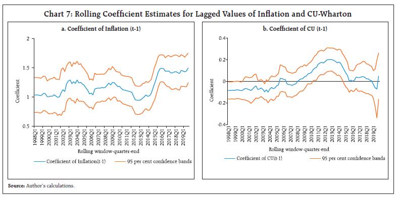In order to check validity of significance of CU coefficients across different sample periods, rolling regressions are estimated with a fixed number of sample observations. The y-o-y inflation is regressed on lagged values of inflation and CU-Wharton as per Model I of Table 5, with a rolling window 40 quarterly observations i.e., data points covering decadal observations covering the entire study period data. The first regression covered period 1988Q2-1998Q1 while last regression tested for ten years sample covering 2010Q1 to 2019Q4. The coefficient of first lag of inflation and CU is presented in Chart 7 along with 95 per cent confidence interval for each of the estimated coefficient. The confidence band includes zero indicating that the coefficient is not statistically different from zero during those phases.

For all rolling windows, the coefficients of lagged inflation values are statistically significant and positive throughout the study period. The chart showing results of lagged coefficient of CU confirms that with change in sample period the statistical significance of coefficient of CU rate, contributing to the behaviour of WPI-manufacturing inflation, also vary. The sign of CU coefficient was negative too for a few sample periods. While for the samples starting from 2000Q3 till 2014Q3, the coefficient of lagged CU was positive and significantly contributed in inflation forecasting through simple regression equation. For other samples, coefficient of CU was although positive, it was not found to be statistically significant. The coefficients of rolling regressions using Model II of Table 5 also follow similar pattern albeit, in little lower ranges. This investigation further confirms that CU rate do influence inflation, but the relationship is not uniform, and it varies with time.

Finally, in the similar manner, the rolling regression is attempted using CU-survey based measure, with rolling window of 35 observations only as entire data series of OBICUS based CU has limited number of observations so far. The first regression covered the sample period 2008Q2-2016Q4 and last regression is tested for the period 2011Q2-2019Q4. Chart 8 represents coefficient lagged OBICUS-CU in case of both the tested models in the study, which clearly indicates that significance of CU coefficient varies with sample and in the later part of sample, especially since 2018Q3, it was not found to be statistically significant in forecasting WPI-manufacturing based inflation, both for y-o-y as well as q-o-q basis.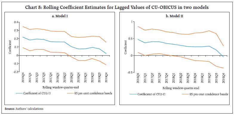

This indicates use of the aggregate economy-wide capacity utilization measure in isolation is less useful as a predictor of inflation. And findings confirm the inferences drawn by Dotsey and Stark (2005), which also applies in Indian context that the impact of CU on inflation is not uniform, and the relationship is conditional on economic circumstances. An analysis including other influencing economic factors such as technological changes, energy prices, unemployment, monetary policy stance etc., might provide additional inputs in further unfolding the historic path of linkages between utilization of capacity and inflation.

V. Conclusion

The OBICUS based CU rate in manufacturing sector provides useful insights into demand pressure in an economy, and also exhibit positive correlation with WPI manufacturing based inflation. At the same time, the long time series of CU, computed using Wharton method, granger causes price change, and provides additional information that the correlation between cyclical components of CU and price levels varies over period. The study also finds that the amplitude of CU cycle was larger in expansion phase than in the contraction phase while the average duration of a complete cycle (trough to trough) was about 14 quarters. The investigation confirms that although CU rate relates to prices both at the level as well as the inflation (rate of change in prices), the relationship varies with time.

The analysis concludes that while the movement in CU primarily shows impact of demand conditions, it also contains information for future inflationary pressures. Using information on CU, in addition to other factors such as technological changes, energy prices, unemployment, monetary policy stance etc., may add value to the inflation forecasting abilities of models.

Reference

Bry, G. and C. Boschan (1971): Cyclical Analysis of Time Series: Selected Procedures and Computer Programs, National Bureau of Economic Research, New York.

Corrado, C. and J. Mattey (1997): Capacity Utilisation, The Journal of Economic Perspectives- American Economic Association, 11(1), 151-167.

Dotsey, M and T. Stark (2005): The Relationship between Capacity Utilization and Inflation, Business Review, Q2 2005, www.philadelphiafed.org.

Benan, E (2011): Alternative Measures of Rate of Capacity Utilisation for the Turkish Economy: A Comparative Analysis in Means of Adequacy for Empirical Investigation and Growth Models, Sosyoekonomi/2011-2.

Finn, Mary G (1996): A Theory of the Capacity Utilisation/Inflation Relationship, Federal Reserve Bank of Richmond Economic Quarterly Volume 82/3.

Harding, D. and A. Pagan (2002): Dissecting the Cycle: A Methodological Investigation, Journal of Monetary Economics, 49(2), 365-381.

Keynes, John Maynard (1936): The General Theory of Employment, Interest, and Money, (New York: Harcourt, Brace and Company).

Mohanty, J., Singh, B., & R. Jain (2003): Business Cycles and Leading Indicators of Industrial Activity in India, MPRA Paper No. 12149, University Library of Munich, Germany.

Mukherjee, A and R. Misra (2012): Estimation of Capacity Utilisation in Indian Industries: Issues and Challenges, RBI Working Paper Series, May

Raj, J., Sahoo, S. and S. Shankar (2018): India’s Investment Cycle: An Empirical Investigation, RBI Working Paper Series, October.

Reserve Bank of India (2006): Report of the Technical Advisory Group on Development of Leading Economic Indicators for Indian Economy, December 1.

Stock, J.H. and M.W. Watson (1999): Forecasting Inflation, Journal of Monetary Economics, vol. 44 (2), October 1999, pp. 293-335.

Annex

Test for Structural Break CU-Wharton series

Dependent Variable: CU-Wharton Series

Sequential F-statistic determined breaks : 1

Breaking variables: C

Sample: 1988Q2 2019Q4

Break test options: Trimming 0.15, Max. breaks 5

^* Prepared by Vijaya Gangadaran and Supriya Majumdar of the Division of Enterprise Surveys, Department of Statistics and Information Management. The views expressed in this article are those of the authors and do not represent the views of the Reserve Bank of India. Authors acknowledge the initial work done by Divya Gupta toward development of a long time series of CU, who worked as a Research Intern in the division for a short duration in 2019. The latest round of the survey data was released on April 7, 2021 on the RBI’s website at https://www.rbi.org.in/Scripts/PublicationsView.aspx?id=20353. The previous article was published in September 2016 issue of the RBI Bulletin and can be accessed at https://www.rbi.org.in/Scripts/BS_ViewBulletin.aspx?Id=16449.

¹ For details of country practices, select literature review of work done in Indian context and CU computation different methods refer to Mukherjee and Misra (2012).

² The methodology of aggregation of survey responses and computation of CU was changed in 2017. The earlier methodology was published in the December 2011 issue of the Reserve Bank’s Bulletin (link- https://www.rbi.org.in/Scripts/BS_ViewBulletin.aspx?Id=12775) while details about current method was published in RBI press release dated October 4, 2017 and available at https://www.rbi.org.in/scripts/PublicationsView.aspx?Id=18031.

³ The trend component in IIP has been removed using Hodrick-Prescott (HP) filter method.

⁴ The analysis in this article, which aims to study the long-run relationship between CU and inflation, is confined to pre-COVID-19 period only as data series used in the study were severely impacted due to pandemic.

⁵ A long time series of IIP-manufacturing with latest base year (2011-12) is constructed using data series for 4 base years viz., 1980-81,1993-94, 2004-05 and 2011-12 by applying linking factor computed by ratio method. Using same method, time series for WPI-manufacturing is constructed using data series for base years 1981-82, 1993-94, 2004-05 and 2011-12.