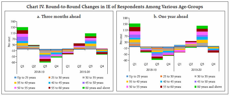
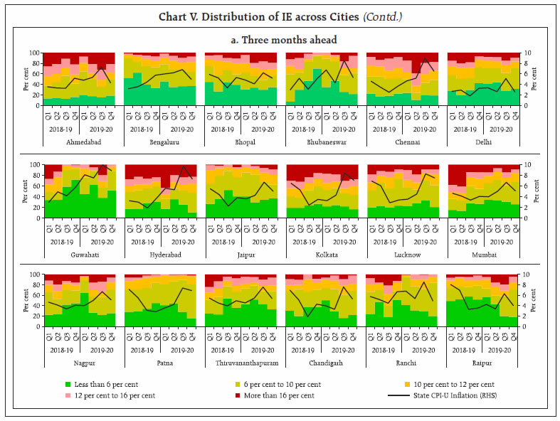
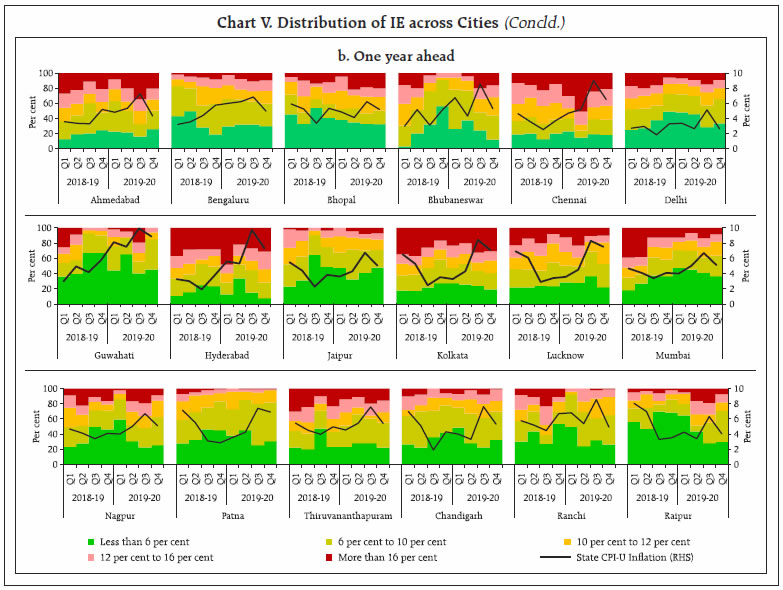
Inflation expectations of households are found to be highly sensitive to actual inflation in India, with specific attributes of households such as their age profile, profession and geographic location contributing variations in formation of expectations. This article derives inflation forecasts from recent data on inflation expectations using two methods: (i) correcting for time varying bias in expectations and (ii) posterior mean. A simple average of such derived forecasts appears to perform better in tracing the likely evolution of actual inflation relative to the individual forecasts. Introduction Survey based information on inflation expectations (IE) of households provide useful inputs for the conduct of monetary policy. It can potentially help assess the future wage-setting behaviour and likely changes in households’ financial decision-making. The Reserve Bank of India has been conducting the Inflation Expectations Survey of Households (IESH) since September 2005, which elicits qualitative and quantitative responses of households’ expectations on changes in price levels and inflation for three months and one year ahead periods. Presently, the survey is conducted in 18 cities and covers about 6,000 households in each round. Households constituting the major share of consumption demand in the economy, their experiences of inflation and expectations about the outlook on future inflation assume vital importance for policy making. This article attempts a comparative study of two existing methodologies, viz., by correcting for time varying bias in IE and by estimating the mean of posterior distribution for given prior information on IE. The remainder of this article is organised as follows. Section II presents recent trends in household IE followed by an overview of the variations observed in IE across demographic groups during 2018-191 and 2019-20 in Section III. Inflation forecasts using IE and their performance in recent period is studied in Section IV. Section V summarises the findings of the study. II. Recent Trends in Households’ Inflation Expectations This section discusses households’ expectations on general prices vis-à-vis movements in Consumer Price Index-Urban2 (CPI-U). The net response on general price levels3 for both three months and one year ahead horizons during 2019-20 witnessed a gradual rise, broadly in-sync with the movement of CPI-U index (Chart Ia). In Q3:2019-20, vegetable prices picked up sharply but declined in the next quarter. This contained worsening of households’ outlook on food prices in this period. The rise in transportation and communication prices in CPI-U during the same period impacted households’ expectations on the cost of services (Annex, Charts A(i) to A(v)). Households’ sentiments on general inflation4 fluctuated widely during 2019-20 (Chart Ib). The net response on the rate of increase of general prices5 for both three months and one year ahead horizons reached its peak in Q3:2019-20. However, it mellowed subsequently on the back of sharp drop in vegetable inflation. Households’ outlook on non-food inflation also took a sharp upturn in the third quarter of 2019-20, partly due to higher inflation in petrol and diesel, which moved from negative to positive territory (Annex, Charts B(i) to B(v)). 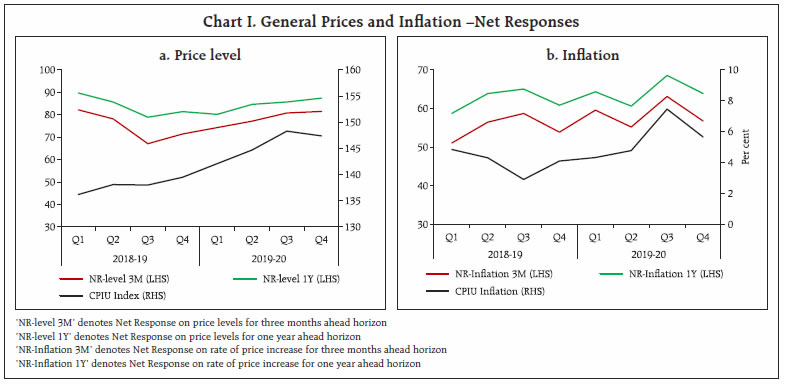 Households’ median IE, which was exhibiting a declining trend since Q3:2018-19, registered an uptick in Q2:2019-20 on the back of mounting food inflation. Median inflation expectations rose by 70 basis points for the next three months and by 90 basis points for a year ahead in Q4:2019-20 over Q4:2018-19. The gap between median inflation perception and the expectations widened, especially for one year ahead, during the second half of 2019-20 (Chart II). The inflation perceptions and expectations broadly tracked the CPI-U inflation during the study period. III. Households’ Attributes Versus Differential in Inflation Expectations Consumers react differently to changes in prices and so is their behaviour in forming inflation expectations and future economic plans. The variation in attitudes impacts their buying, consumption and investment patterns, which in turn contribute to future inflation. Perceptions, expectations as well as attitudes towards prices are required to be captured on a continuous basis (Mueller, 1959). The differentials in IE among various categories of consumers impact the economy through various channels, e.g., asset market models, investments, etc. (Gnan et al., 2011). The errors in forecasts of economic variables by consumers in Michigan survey6 are systematically correlated with their demographic characteristics (Souleles, 2004). In the Indian context, it is recognised that heterogeneity across various categories of households has an impact on formation of inflationary expectations (Goyal and Parab, 2019). To understand the influence of the demographic characteristics of respondents on households’ IE, this article has examined the variations in IE across different occupation groups and age profile of respondents for the recent period. Looking at the round-to-round percentage changes in median IE of different groups of respondents, it is found that changes in IE were mostly broad-based in the same direction (Chart III). In recent period, fluctuations in overall three months ahead and one year ahead IE largely occurred on the back of variation in sentiments of financial sector employees. On the other hand, respondents in the age group of 55 to 60 years contributed the most to changes in three months ahead IE and the movements in one year ahead IE were driven by respondents in 50 to 55 years and 55 to 60 years age groups (Chart IV). The city-wise variation in the respondents’ outlook on future inflation was studied by classifying the quantitative IE under five groups, viz., ‘less than 6 per cent’, ‘6 per cent to 10 per cent’, ’10 per cent to 12 per cent’, ‘12 per cent to 16 per cent’ and ‘more than 16 per cent’. For each city, the percentage of respondents with IE in these groups’ and the corresponding state’s CPI-U inflation (during the survey month) over the survey rounds of 2018-19 and 2019-20 are plotted in Chart V. A sharp rise was observed in the realised CPI-U inflation in most of the states during Q3:2019-20. As a result, respondents in most of the survey centres shifted their IE to the highest inflation bracket during the period. This was more prominent in Ahmedabad, Chennai, Hyderabad and Kolkata. Differentials in households’ inflation outlook seen above, across different respondent groups and geographic locations, may be attributed to their differences in collecting and assimilating the information while forming the expectations (Gnan et al., 2011). 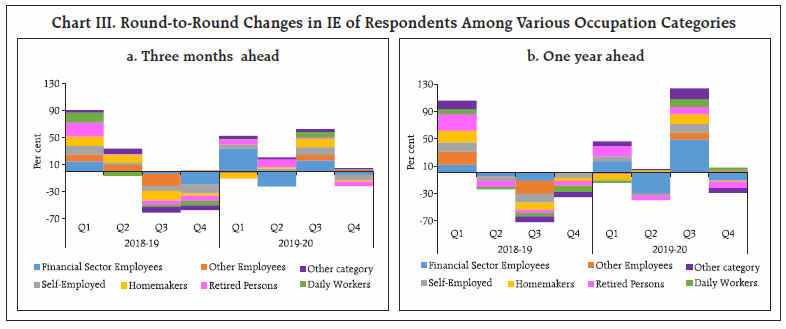
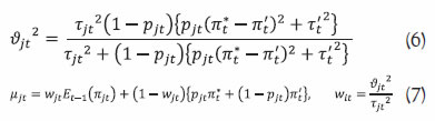
 IV. Inflation Forecasts Derived from Inflation Expectations Among the several objectives of capturing households’ IE, one important purpose is to attain an idea about futuristic inflation. For this purpose, however, IE should be rational and as a crucial condition of rationality must pass the test of unbiasedness. According to recent empirical research, this condition is not satisfied in the Indian context (Shaw, 2019). Assuming the bias (ett-1) to be time-varying as shown in equation (1) below, an autoregressive (AR) model as per equation (2), helps in predicting the future bias in expectations (hereafter referred to as “Adjustment using Time Varying Bias Prediction Method (ATVBPM)”) (Kim and Kim, 2009). The IE for the future period is then corrected for the predicted bias and the resulting estimate provides an inflation forecast. Further, by studying households’ IE in the Indian context from Q2:2008-09 to Q4:2018-19, it has been proved that ‘ATVBPM’ improves the degree of accuracy of inflation forecasts (Shaw et al., 2019). 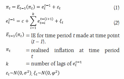 Alternatively, Shaw (2019) used a method suggested by Batchelor (2006) to convert IE into rational IE (hereafter referred as “Posterior Mean (PM)”) and found that it results in efficient inflation forecasts. This procedure postulates models given in equations (3) and (4) and derives the posterior distribution of inflation given the IE as shown in equation (5) with parameters given in equations (6) and (7). The estimate of the posterior mean (µjt) gives inflation forecast for the period t. 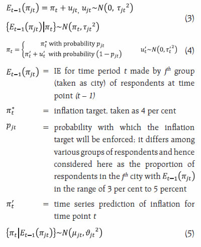
 The following analysis checks robustness of earlier findings for recent periods and examines empirically the efficacy of the forecast combination, through simple average. Following ‘ATVBPM’ and ‘PM’ and using three months ahead mean IE, one quarter ahead out-of-sample CPI Combined7 (CPI-C) inflation forecasts are computed for the period Q2:2017-18 to Q4:2019-20. Besides, in this article, average forecasts (‘AVG’) based on ‘ATVBPM’ and ‘PM’ are also computed. These inflation forecasts are then compared with the inflation forecasts obtained based on ‘Random Walk (RW)’ with drift and ‘AR(1)’ models. Keeping ‘RW’ model as the benchmark, the Relative Average Absolute Deviations (‘RAADM’), given in equation (8), identifies a better model for forecasting. Lower the value of RAADM, better is the model ‘M’ for forecasting inflation, in comparison to the benchmark model ‘RW’. 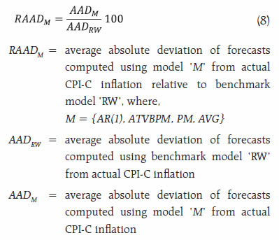
| Table 1. Performance of Inflation Forecasts | | Method | RAAD | | Auto Regressive Model: AR(1) | 93.07 | | Adjustment using Time Varying Bias Prediction Method (ATVBPM) | 92.75 | | Posterior Mean (PM) | 83.21 | | Average of ATVBPM and PM (AVG) | 82.14 | Table 1 and Chart 6 show that inflation forecasts obtained by taking the average of forecasts from ‘ATVBPM’ and ‘PM’ perform better than the individual forecasts as shown by the lowest value of ‘RAADM’ for average forecasts. V. Conclusion This study analyses the formation of households’ inflation expectations and finds that households’ inflation sentiments have been highly influenced by their experiences of the actual inflation. Households’ attributes such as the age-profile and profession are found to contribute to differences observed in the formation of inflation expectations. As inflation expectations seem to contain lead information about plausible inflation trajectory, this article converts survey-based inflation expectations to inflation forecasts using two existing methodologies, viz., correcting for time varying bias in expectations and posterior mean as well as a combination of individual forecasts. The average of forecasts is found to provide better forecasts in terms of both the direction and magnitude of change in actual inflation. Further, future research covering whole range of alternative methodologies and over a longer time horizon could help ensure robustness of the findings. References Batchelor, R. (2006), “How robust are quantified survey data?”, Evidence from the United States. Cass Business School, City of London. Gnan, E., Langthaler, J., and Valderrama, M. T. (2011), “Heterogeneity in Euro Area Consumers’ Inflation Expectations: Some Stylized Facts and Implications”, Monetary Policy and the Economy, Q2(11):43–66. Goyal, A., and Parab, P. (2019), “Modelling Heterogeneity and Rationality of Inflation Expectations across Indian Households”, Indira Gandhi Institute of Development Research WP-2019-002. Kim, I., and Kim, M. (2009), “Irrational Bias in Inflation Forecasts”, Munich Personal RePEc Archive Paper 16447, University Library of Munich, Germany. Mueller, E. (1959), “Consumer Reactions to Inflation”, The Quarterly Journal of Economics, 73(2), 246-262. Shaw, P. (2019), “Using Rational Expectations to Predict Inflation”, Reserve Bank of India Occasional Papers, 40(1):85-104. Shaw, P., Jayaraman, A. R., and Das, T. B. (2019), “Households’ Inflation Expectations: A Reflection”, Reserve Bank of India Bulletin, December, 2019:59-69 Souleles, N. S. (2004), “Expectations, Heterogeneous Forecast Errors, and Consumption: Micro Evidence from the Michigan Consumer Sentiment Surveys”, Journal of Money, Credit and Banking 36(1): 39-72.
Annex - Charts
|