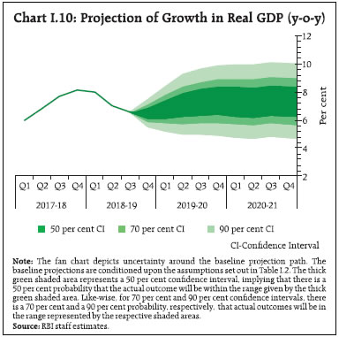
| I. Macroeconomic Outlook The macroeconomic setting for the conduct of monetary policy has undergone significant shifts as domestic activity lost speed in 2018-19 and inflation conditions turned unusually benign under the impact of deflationary food prices. Going forward, economic activity is expected to recover in 2019-20. Headline CPI inflation is projected to move up from its recent lows as the favourable base effects dissipate but remain below the target of 4 per cent in 2019-20. Global economic activity and trade have been shedding momentum and downside risks to the outlook have increased. I.1 Key Developments since October 2018 MPR Since the release of the Monetary Policy Report (MPR) of October 2018, the macroeconomic setting for the conduct of monetary policy has undergone significant shifts. After averaging close to 8 per cent through Q3:2017-18 to Q1:2018-19, domestic economic activity lost speed. The February 2019 release of the Central Statistics Office (CSO), read in conjunction with high frequency indicators, suggests that the economy could have encountered a soft patch. At the same time, some of the forward-looking surveys conducted by the Reserve Bank of India (RBI) indicate that consumer confidence has improved and business expectations remain optimistic. Moreover, aggregate flow of funds to the commercial sector from banks and non-banks remains robust, led by strong growth in bank credit. Inflation conditions have turned unusually benign under the impact of deflationary food prices. While total financial flows from banking and non-banking sources have improved, a durable strengthening of investment demand is yet to take hold. Turning to the international environment, global activity and trade have been shedding momentum and downside risks to the outlook have increased. Tracking other commodity prices, international crude oil prices have declined sharply from their October highs, though they continue to be volatile. Protracted trade tensions and concerns over Brexit have eroded business and consumer confidence in major countries/ regions. In response to these evolving developments, monetary policy authorities across the world have stepped back from further tightening/normalisation, and more recently a more accommodative stance is evident from some central banks. Monetary Policy Committee: October 2018-February 2019 During October 2018-February 2019, the Monetary Policy Committee (MPC) met thrice in accordance with its bi-monthly schedule. The MPC maintained status quo on the policy repo rate in its October 2018 meeting (with a majority of 5-1) but switched stance from neutral to calibrated tightening. The MPC’s decision was conditioned by risks to inflation from volatile crude oil prices; rising input costs; fiscal slippage concerns; uncertainty about the impact of minimum support prices (MSPs); the staggered impact of the likely increase in house rent allowances by the states; and, the virtual closing of the output gap. In its December 2018 meeting, the MPC left the policy rate unchanged and retained the stance of calibrated tightening, although inflation projections were revised downwards. In its February 2019 meeting, the MPC decided to reduce the policy repo rate by 25 basis points (bps) by a majority of 4-2 and was unanimous in voting for switching its stance to neutral from calibrated tightening. This decision was prompted by the continuous easing of headline inflation, a stable crude oil price outlook and some moderation in cost pressures. Headline inflation was projected to remain below the target of 4 per cent over the coming four quarters, which opened up space for easing. The diversity in the MPC’s voting pattern observed during October 2018-February 2019 was also seen in some other central banks (Table I.1), reflecting differences in individual members’ assessments and expectations, and policy preferences. | Table I.1: Monetary Policy Committees and Voting Pattern | | Country | Policy Meetings: October 2018 - March 2019 | | Total Meetings | Meetings With Full Consensus | Meetings With Dissents | | Brazil | 4 | 4 | 0 | | Chile | 4 | 4 | 0 | | Colombia | 4 | 4 | 0 | | Czech Republic | 4 | 0 | 4 | | Hungary | 5 | 5 | 0 | | Israel | 4 | 2 | 2 | | Japan | 4 | 0 | 4 | | South Africa | 3 | 2 | 1 | | Sweden | 3 | 1 | 2 | | Thailand | 4 | 1 | 3 | | UK | 4 | 4 | 0 | | US | 4 | 4 | 0 | | Sources: Central bank websites. | Macroeconomic Outlook Chapters II and III analyse macroeconomic developments during October 2018-March 2019 and explain the deviations of inflation and growth outcomes from staff’s projections. Turning to the outlook, the evolution of key macroeconomic and financial variables over the past six months warrants revisions in the baseline assumptions (Table I.2). First, international crude oil prices have declined sharply from their October 2018 level, even though they have rebounded in recent months. Crude oil prices (Indian basket) fell from their peak of around US$ 85 a barrel in early October 2018 to a low of around US$ 52 at end-December on the back of higher supplies and a slowdown in global demand. Prices edged higher to average around US$ 67 during March, after the Organisation of the Petroleum Exporting Countries (OPEC) and Russia cut production beginning January 2019, and production was disrupted in Venezuela. Given the current demand-supply assessment and signals extracted from the futures market, the baseline scenario assumes crude oil prices at an average of US$ 67 per barrel during 2019-20 (Chart I.1). | Table I.2: Baseline Assumptions for Near-Term Projections | | Indicator | October 2018 MPR | Current MPR (April 2019) | | Crude Oil (Indian basket) | US$ 80 per barrel during H2:2018-19 | US$ 67 per barrel during 2019-20 | | Exchange rate | ₹72.5/US$ | ₹69/US$ | | Monsoon | 9 per cent below LPA in 2018 | Normal for 2019 | | Global growth | 3.9 per cent in 2018 | 3.5 per cent in 2019 | | 3.9 per cent in 2019 | 3.6 per cent in 2020 | | Fiscal deficit (per cent of GDP) | To remain within BE 2018-19
Centre: 3.3
Combined: 5.9 | To remain within BE 2019-20
Centre: 3.4
Combined: 5.9 | | Domestic macroeconomic/ structural policies during the forecast period | No major change | No major change | Notes: 1. The Indian basket of crude oil represents a derived numeraire comprising sour grade (Oman and Dubai average) and sweet grade (Brent) crude oil.
2. The exchange rate path assumed here is for the purpose of generating staff’s baseline growth and inflation projections and does not indicate any ‘view’ on the level of the exchange rate. The Reserve Bank is guided by the objective of containing excess volatility in the foreign exchange market and not by any specific level of and/or band around the exchange rate.
3. Global growth projections are from the World Economic Outlook (July 2018 and January 2019 Updates), International Monetary Fund (IMF).
4. BE: Budget estimates.
5. LPA: Long period average.
6. Combined fiscal deficit refers to that of the Centre and States taken together. Combined fiscal deficit for 2019-20 is assumed to be the same as in 2018-19, as all state governments have not yet presented their budgets.
Sources: RBI staff estimates; Budget documents; and IMF. | Second, the nominal exchange rate (Indian rupee vis-à-vis the US dollar) has appreciated from its October 2018 level, buoyed by the steady revival of portfolio flows, softening of crude oil prices, lower domestic inflation prints, and dovish monetary policy stance in the US. Third, the pace of global economic activity and trade has turned out to be well below earlier expectations on account of elevated trade tensions, tighter financial conditions, uncertainty surrounding Brexit and slowdown in China. The global manufacturing purchasing managers’ index touched a 32-month low in February 2019 and remained weak in March. Global growth in 2019 is expected to be lower than that in the previous two years for both advanced economies (AEs) and emerging market and developing economies (EMDEs) (Chart I.2). I.2 The Outlook for Inflation Headline CPI inflation has declined sharply since mid-2018, driven by the sustained fall in food inflation (even turning into deflation during October 2018-February 2019), the waning away of the direct impact of house rent allowances for central government employees, and more recently, by a sharp fall in fuel inflation. CPI inflation excluding food and fuel has also moderated somewhat, though its level remains elevated. Overall, CPI inflation fell from 3.7 per cent in August-September 2018 to 2.6 per cent in February 2019 after touching a low of 2.0 per cent in January 2019 (Chapter II). 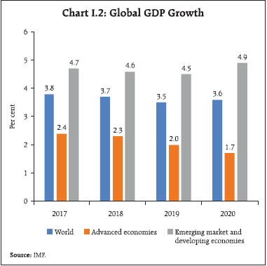 Turning to the outlook for inflation, inflation expectations of households and firms play an important role in shaping future inflation by influencing price and wage contracts. Inflation expectations of urban households surveyed by the Reserve Bank in its March 2019 round1 decreased by 40 bps each over the previous round (December 2018) for the three months ahead and one year ahead horizons to 7.8 per cent and 8.1 per cent, respectively. Three-month ahead inflation expectations in the March 2019 round were lower by 160 bps vis-à-vis the September 2018 round, but were unchanged from the March 2018 round. One-year ahead inflation expectations in the March 2019 round softened by 170 bps and 50 bps from the September 2018 and March 2018 rounds, respectively. The proportion of respondents expecting the general price level to increase by more than the current rate declined for both the three months ahead and one year ahead horizons (Chart I.3). Manufacturing firms polled in the January-March 2019 round of the Reserve Bank’s industrial outlook survey expected a reduction in pressures from the cost of raw materials in Q1:2019-20 (less negative values for cost of raw materials indicate less input price pressures) (Chart I.4).2 The outlook on selling prices remains robust. According to the Nikkei’s purchasing managers’ survey, firms in the manufacturing sector (March 2019) and services sector (February 2019) reported some moderation in pressures on both input and output prices. Professional forecasters surveyed by the Reserve Bank in March 2019 expected CPI inflation to increase from 2.6 per cent in February 2019 to 4.2 per cent by Q4:2019-20 (Chart I.5).3 Taking into account the initial conditions, signals from forward-looking surveys and estimates from structural and other models (Box I.1), CPI inflation is projected to pick up from 2.6 per cent during February 2019 to 2.9 per cent in Q1:2019-20, 3.0 per cent in Q2, 3.5 per cent in Q3, and 3.8 per cent in Q4, with risks broadly balanced (Chart I.6). The 50 per cent and the 70 per cent confidence intervals for headline inflation in Q4:2019-20 are 2.5-5.2 per cent and 1.7-5.9 per cent, respectively. For 2020-21, assuming a normal monsoon and no major exogenous or policy shocks, structural model estimates indicate that inflation will move in a range of 3.8-4.1 per cent. The 50 per cent and the 70 per cent confidence intervals for Q4:2020-21 are 2.6-5.7 per cent and 1.8-6.5 per cent, respectively. There are a number of upside and downside risks to the baseline inflation forecasts. The major upside risks include: geopolitical tensions and supply disruptions in the global crude oil market; volatility in international and domestic financial markets; the risk of a sudden reversal in the prices of volatile perishable food items; and, fiscal slippages. Among the downside risks are: a sharper than anticipated slowdown in global growth and its softening impact on crude oil and other commodity prices; and the persistence of a food supply glut keeping headline inflation below the baseline path. Box I.1: Output Gap and Core Inflation An accurate forward-looking assessment of inflation dynamics and their macroeconomic drivers is critical for the effective conduct of monetary policy in a flexible inflation targeting (FIT) regime. Inflation ultimately reflects demand-supply imbalances in the economy. The Phillips curve relates movements in inflation to the output gap4 as a proxy for demand-supply mismatches and suggests a trade-off between inflation and output in the short run, i.e., any attempt to boost economic activity (above its potential or capacity) can intensify inflationary pressures; similarly, any policy action intended to contain inflation will involve some temporary sacrifice of output. The Phillips curve relationship, which lies at the core of modern monetary theory and policy, has come under scrutiny over the past decade in view of inflation being largely impervious to large swings in economic activity and employment, especially in major advanced economies. These developments have lent credence to the argument that the curve has flattened or may even be dead reflecting, inter alia, the well-anchored inflation expectations, increased global integration, and uncertainty about the true output gap (Hooper et al., 2019). Another view is that the relationship may be non-linear (convex): inflation is less responsive to low or negative values of the output gap but could be highly sensitive to a large and increasing positive output gap. This could be due to the downward rigidity in wages and prices, which dampens the impact of low or negative output gaps on wages/prices and hence inflation. The non-linearity could also occur if there is a decline in trend inflation, as a result of which firms adjust prices less frequently implying a flatter Phillips curve, and a steeper curve for an increase in trend inflation (Ball et al., 1988). In emerging markets like India, the Phillips curve framework continues to be relevant for the conduct of monetary policy, despite recurrent and large supply shocks (Patra et al., 2017). The Phillips curve is a key pillar of the RBI’s workhorse Quarterly Projection Model (QPM)5 (Benes et al., 2016). In the QPM, core inflation (i.e., inflation excluding food and fuel) depends on: (a) the output gap; (b) expected inflation as well as its past values to capture both the forward-looking and the adaptive (backward-looking) components of the inflation process; (c) the real exchange rate: as depreciation raises the domestic cost of imported intermediate inputs and final goods, there is upward pressure on domestic prices; and, (d) domestic food and fuel prices. Taking various interactions, feedbacks and policy reactions within the QPM, a positive shock to the output gap increases core and headline inflation and the peak effect occurs with a lag of 3-5 quarters, the impact being stronger and faster for core inflation than for headline inflation (Chart I.1.1). 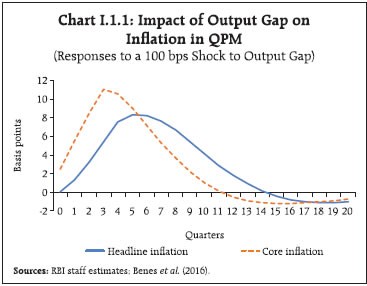 As noted earlier, the relationship between inflation and the output gap could be non-linear, with the impact of the output gap increasing more than proportionally as it turns positive. Accordingly, the following equation for core inflation is estimated using an exponential formulation for the output gap term: Note: Figures in parentheses are p-values. The results indicate that the Phillips curve is relatively flat for negative output gaps, but the impact increases rapidly with positive output gaps (Chart I.I.2). Such a relationship could occur if, for instance, the pricing power increases more than proportionally with the strengthening of economic activity. The results suggest the need for monetary policy to be vigilant in times of large positive output gaps. References: Ball, L., N.G. Mankiw, and D. Romer (1988), “The New Keynesian Economics and the Output-Inflation Trade-off”, Brookings Papers on Economic Activity, 1988(1), 1-82. Benes, J., K. Clinton, A. George, P. Gupta, J. John, O. Kamenik, D. Laxton, P. Mitra, G. Nadhanael, R. Portillo, H. Wang, and F. Zhang (2016), “Quarterly Projection Model for India: Key Elements and Properties”, RBI Working Paper Series No. 08. Hooper, P., F. Mishkin, and A. Sufi (2019), “Prospects for Inflation in a High Pressure Economy: Is the Phillips Curve Dead or is It Just Hibernating?”, US Monetary Policy Forum 2019. Patra, M. D., J.K. Khundrakpam, and S. Gangadaran (2017), “The Quest for Optimal Monetary Policy Rules in India”, Journal of Policy Modeling, 39(2), 349-370. | Inflation forecasts are critical for the conduct of forward-looking monetary policy and they play a special role in an inflation targeting framework by acting as an intermediate target. An analysis of cross-country forecast errors indicates that there is a positive correlation of the errors with the share of food in the CPI basket (Box I.2). I.3 The Outlook for Growth As noted earlier, economic activity weakened in the second half of 2018-19. Looking ahead, favourable factors such as an increase in financial flows to the commercial sector, stabilisation of crude oil and other commodity prices, consumption- and investment-enhancing proposals in the Union Budget 2019-20, and, the expectation of a normal monsoon are expected to boost economic activity. However, there could be headwinds from greater than expected moderation in global growth and global trade as well as unanticipated volatility in global financial markets. Turning to the forward-looking surveys, consumer confidence a year ahead has increased considerably in the March 2019 round of the Reserve Bank’s survey on positive sentiment pertaining to the general economic situation and the employment scenario (Chart I.7).8 Overall optimism in the manufacturing sector for the quarter ahead registered some moderation in the March 2019 round of the Reserve Bank’s industrial outlook survey due to some dip in prospects for production, order books, exports, and capacity utilisation (Chart I.8). Surveys by other agencies indicate a mixed picture on future business expectations (Table I.3). Firms in the manufacturing and services sectors polled in the Nikkei’s purchasing managers’ survey were optimistic about one-year ahead output prospects. In the March 2019 round of the Reserve Bank’s survey, professional forecasters expected real GDP growth to recover from 6.6 per cent in Q3:2018-19 to 7.5 per cent in Q4:2019-20 (Chart I.9). Taking into account the baseline assumptions, survey indicators, the cut in the policy repo rate in the February 2019 policy and model forecasts, real GDP growth is projected to improve from 7.0 per cent in 2018-19 to 7.2 per cent in 2019-20 – 6.8 per cent in Q1, 7.1 per cent in Q2, 7.3 per cent in Q3, and 7.4 per cent in Q4 – with risks evenly balanced around this baseline path (Table I.4). For 2020-21, the structural model estimates indicate real GDP growth at 7.4 per cent, with quarterly growth rates in the range of 7.3-7.5 per cent, assuming a normal monsoon, and no major exogenous or policy shocks. There are upside as well as downside risks to the baseline growth scenario (Chart I.10). The boost to private investment activity from faster resolution of stressed assets and increased as well as more broad-based credit offtake amidst rising capacity utilisation can raise the baseline growth projection. Conversely, further escalation of trade tensions and protectionist trends, increased volatility in global financial conditions over the uncertainty of the stance of monetary policy in the US and other advanced economies, uncertainty surrounding Brexit, a sharper slowdown in the Chinese economy and deviations of the south-west monsoon from the baseline assumption of a normal monsoon may pose downside risks to the baseline growth path. Box I.2: RBI Inflation Forecasts – An Evaluation RBI’s bi-monthly resolutions provide inflation forecasts for up to four quarters ahead. The Monetary Policy Report (MPR), released twice a year (April and October), provides inflation forecasts up to eight quarters ahead. Inflation forecasts for the period from April 2015 to September 2018 for up to four quarters ahead are benchmarked vis-à-vis those of some major central banks. Inflation in India eased significantly for a few months following demonetisation, which imparted a large upward bias to the forecasts made prior to November 2016 and for a few subsequent months. The analysis, therefore, presents results for the full sample period as well as for the period excluding demonetisation. The sample period also includes the introduction of the goods and services tax – a major structural reform measure – in July 2017 which, as the cross-country evidence suggests, adds uncertainty to the inflation outlook during the implementation stage. The mean forecast error for the sample excluding the demonetisation period is (-) 30 bps9 as compared with a range of 0 to (-) 40 bps for the other sample countries (Table I.2.1).10 The standardised mean error (i.e., the mean error divided by the respective inflation targets of the sample countries) is around 8 per cent for India vis-à-vis 0-13 per cent for the sample countries. Similarly, the mean absolute forecast error and the root mean squared error for RBI forecasts are within the ranges observed for the sample countries. | Table I.2.1 Inflation Forecast Errors | | (Percentage points) | | Item | India (full sample) | India (sample excluding October 2016-June 2017) | UK | Czech Republic | Sweden | Hungary | | Mean Error (ME) | -0.7 | -0.3 | 0.0 | 0.0 | 0.0 | -0.4 | | Standardised ME | -18.4 | -7.7 | -0.2 | 0.5 | 0.6 | -12.6 | | Mean Absolute Error (MAE) | 0.8 | 0.4 | 0.2 | 0.4 | 0.3 | 0.6 | | Standardised MAE | 20.7 | 10.7 | 11.6 | 19.3 | 14.6 | 19.6 | | Root Mean Squared Error (RMSE) | 1.1 | 0.6 | 0.3 | 0.5 | 0.4 | 0.8 | | Standardised RMSE | 27.6 | 13.8 | 14.2 | 24.3 | 17.6 | 27.2 |  | The share of food in the CPI basket varies widely across countries, which could have a significant bearing on forecast errors. Absolute measures of errors are found to be correlated with the share of food items in the CPI. There is a considerable flattening of the relationship once the forecast errors are standardised with respective inflation targets (Chart I.2.1). A desirable characteristic of a good forecast is that it should be unbiased, i.e., on average, the forecast error should be zero. Unbiasedness can be tested by regressing forecast errors on a constant by estimating the following equation:
| Table I.2.2: Unbiasedness Test | | Forecast horizon | India (full sample) | India (sample excluding October 2016-June 2017) | Czech Republic | Hungary | Sweden | UK | | 1 quarter ahead | -0.30** | -0.11 | 0.07 | -0.15 | -0.01 | -0.02 | | | (0.03) | (0.24) | (0.43) | (0.24) | (0.74) | (0.36) | | 2 quarters ahead | -0.64*** | -0.34** | 0.09 | -0.27 | 0.02 | -0.01 | | | (0.00) | (0.03) | (0.57) | (0.17) | (0.76) | (0.93) | | 3 quarters ahead | -0.88*** | -0.27 | -0.03 | -0.49 | 0.04 | -0.02 | | | (0.00) | (0.11) | (0.83) | (0.10) | (0.68) | (0.87) | | 4 quarters ahead | -1.13*** | -0.51*** | -0.09 | -0.60 | -0.00 | 0.03 | | | (0.00) | (0.01) | (0.63) | (0.10) | (0.99) | (0.86) | Notes: Figures in parentheses are p-values.
***,**,*: Significant at <1%, <5% and <10% levels, respectively.
Sources: Central bank websites; RBI staff estimates. | Reference: Raj, J., M. Kapur, P. Das, A. George, G. Wahi and P. Kumar (2019), “Inflation Forecasts: Recent Experience in India and a Cross Country Assessment”, Reserve Bank of India (Mimeo). | I.4 Balance of Risks The baseline projections of growth and inflation presented in the previous sections are based on a set of assumptions explained in Table I.2. However, there are substantial uncertainties around these baseline assumptions which pose risks, both upside and downside, to the baseline projections. The projected paths of growth and inflation under various plausible alternative scenarios are discussed below: (i) Global Growth Uncertainties Global growth and trade have surprised on the downside in recent quarters. The baseline scenario in Table I.2, therefore, assumes some slowdown in global growth in 2019 vis-à-vis preceding years. However, global growth could turn out to be even lower on further escalation of trade tensions, volatility in global financial markets, more-than-envisaged slowdown in the Euro area and China, and limited monetary and fiscal policy space in major countries. In such circumstances, if global growth turns out to be 50 bps below the baseline, domestic GDP growth and inflation could be lower by around 15-20 bps and 10 bps, respectively, below the baseline. On the other hand, an orderly and quick resolution of trade issues between the US and China, and more accommodative monetary policies in the major advanced economies than currently anticipated on the back of a benign inflation outlook, could provide support to the global economy. Should global growth turn out to be 50 bps above the baseline scenario, domestic growth and inflation could be around 15-20 bps and 10 bps above the baseline (Charts I.11 and I.12).
| Table I.3: Business Expectations Surveys | | Item | NCAER Business Confidence Index (March 2019) | FICCI Overall Business Confidence Index (February 2019) | Dun and Bradstreet Composite Business Optimism Index (January 2019) | CII Business Confidence Index (March 2019) | | Current level of the index | 127.0 | 60.3 | 73.8 | 65.2 | | Index as per previous survey | 133.1 | 61.9 | 79.5 | 61.8 | | % change (q-o-q) sequential | -4.6 | -2.6 | -7.2 | 5.5 | | % change (y-o-y) | -1.8 | -15.8 | -18.9 | 8.7 | Notes: 1. NCAER: National Council of Applied Economic Research.
2. FICCI: Federation of Indian Chambers of Commerce & Industry.
3. CII: Confederation of Indian Industry. |
| Table I.4: Projections - Reserve Bank and Professional Forecasters | | (Per cent) | | | 2018-19 | 2019-20 | 2020-21 | | Reserve Bank’s Baseline Projections | | | | | Inflation, Q4 (y-o-y) | 2.4 | 3.8 | 4.1 | | Real GDP growth | 7.0 | 7.2 | 7.4 | | Median Projections of Professional Forecasters | | | | | Inflation, Q4 (y-o-y) | 2.4 | 4.2 | | | Real GDP growth | 7.0 | 7.3 | | | Gross domestic saving (per cent of GNDI) | 29.9 | 30.2 | | | Gross fixed capital formation (per cent of GDP) | 29.0 | 29.4 | | | Credit growth of scheduled commercial banks | 13.8 | 13.3 | | | Combined gross fiscal deficit (per cent of GDP) | 6.4 | 6.3 | | | Central government gross fiscal deficit (per cent of GDP) | 3.4 | 3.4 | | | Repo rate (end-period) | 6.25 | 6.00 | | | Yield on 91-days treasury bills (end-period) | 6.3 | 6.1 | | | Yield on 10-year central government securities (end-period) | 7.4 | 7.3 | | | Overall balance of payments (US$ billion) | -13.6 | 11.4 | | | Merchandise export growth | 8.0 | 5.6 | | | Merchandise imports growth | 10.5 | 6.0 | | | Current account balance (per cent of GDP) | -2.4 | -2.3 | | GNDI: Gross National Disposable Income.
Source: RBI staff estimates; and Survey of Professional Forecasters (March 2019). |
 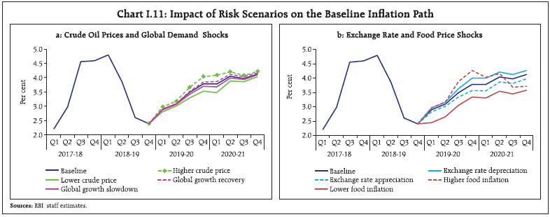 (ii) International Crude Oil Prices Global crude oil prices have declined sharply from their October 2018 levels; however, the short- and medium-term outlook remains uncertain. If oil supply becomes constricted due to geopolitical tensions and continuing OPEC production cuts, there could be a sudden and large upward pressure on oil prices. Assuming an increase in the Indian basket crude oil prices to around US$ 77 per barrel, inflation could be higher by 30 bps and growth could be weaker by around 20 bps. On the other hand, if global economic activity disappoints more than expected for the earlier noted reasons, crude oil demand could be lower. Moreover, the effectiveness of production cuts by the OPEC may be impaired if there is a compensating increase in shale output. If the Indian basket crude price were to fall to US$ 57 per barrel, inflation could ease by around 30 bps, with a boost of around 20 bps to growth. (iii) Exchange Rate The nominal exchange rate of the Indian rupee vis-à-vis the US dollar has appreciated from its October level, after coming under sustained pressure during August-September 2018. Higher crude oil prices and volatility in portfolio flows could put downward pressure on the Indian rupee. A depreciation of the Indian rupee by around 5 per cent relative to the baseline could increase inflation by around 20 bps, while providing a boost of 15 bps to growth. Conversely, India’s sound domestic fundamentals and increased capital inflows can lead to an appreciation of the domestic currency. An appreciation of the Indian rupee by 5 per cent could soften inflation by around 20 bps and lower growth by around 15 bps. (iv) Food Inflation Food inflation in India remained softer than expected in 2018-19, dipping into negative territory during October 2018-February 2019. Domestic food production is at historically high levels. The baseline path assumes food inflation to edge higher, with the dissipation of base effects. Going forward, adequate buffer stocks in cereals, a favourable demand-supply balance in many food items and continuing low global food prices could keep food inflation under check in 2019-20. Owing to these factors, should food inflation remain below the projected path by 100 bps, headline inflation may remain below the baseline by up to around 50 bps. On the other hand, given the unusually low food inflation, there is a risk of a sudden reversal in the prices of perishable food items. Should the monsoon be deficient, this may reduce agricultural production and exert upward pressure on food prices. In this scenario, GDP growth could be lower by around 30 bps in 2019-20, and higher food prices may push up headline inflation above the baseline by around 50 bps by the end of 2019-20. (v) Fiscal Slippages In 2018-19, the Centre’s indirect tax collections trailed budget estimates and contributed to the fiscal deficit turning out to be higher in the revised estimates. The baseline projections assume a fiscal stance as announced in the budgets for 2019-20. Going forward, alternative farm support schemes and farm loan waivers announced by some state governments, higher minimum support prices and food procurement, and lower direct tax collections could put upward pressure on the combined fiscal deficit. Should there be a fiscal slippage on account of such factors, this could crowd out private investment, impact potential output, and result in higher inflation. Conversely, with the stabilisation of the GST, indirect tax revenues could improve more than currently budgeted, which could help contain deficits, and provide higher resources for private investment, enhance potential output and reduce inflation. I.5 Conclusion To sum up, headline CPI inflation is expected to move up from its recent lows as the favourable base effects dissipate but is expected to remain below the target of 4 per cent. Higher crude oil prices, volatility in international financial markets, the risk of a sudden reversal in the prices of perishable food items, and fiscal slippages are, however, upside risks to the inflation trajectory. Softer crude oil and commodity prices on the back of a sharper slowdown in global growth, and the persistence of low food inflation pose downside risks to the headline inflation path. Real GDP growth is expected to recover in 2019-20. Private consumption is likely to remain its mainstay and investment activity is expected to remain strong. Recapitalisation of public sector banks and the ongoing improvement in their financials, and resolution of stressed assets under the insolvency and bankruptcy code are expected to improve bank credit offtake and support investment and aggregate demand. The policy repo rate cut in February 2019 and the demand-enhancing proposals in the Union Budget 2019-20 are also expected to boost aggregate demand. Deceleration in global trade and global GDP growth, however, poses downside risks to domestic economic activity. _________________________________________________________
II. Prices and Costs Consumer price inflation has weakened in a broad-based manner with food prices contracting for five consecutive months since September 2018, fuel inflation collapsing and inflation excluding food and fuel softening even though it remains at an elevated level. Nominal growth in rural wages for both agricultural and non-agricultural labourers remained muted and pressure from staff costs in the organised sector was range-bound in Q3:2018-19. Industrial and farm input costs moderated considerably. Consumer price index (CPI) inflation surprised on the downside in Q4:2018-19, falling to 2.0 per cent in January 2019, the legislated floor for CPI inflation.1 It was the lowest reading since June 2017 when it briefly fell to 1.5 per cent. Although it edged up in February, its momentum remained weak relative to expectations. Prices of food and beverages contracted for five consecutive months since September 2018 leading to the longest deflationary spell in these prices in the CPI series so far. Fuel and light inflation collapsed from its recent peak in September tracking the softness in international energy prices and the unusual sharp decline in electricity prices. Inflation in CPI excluding food and fuel also softened since October with the statistical impact of the increase in house rent allowances (HRA) for central government employees on headline inflation dissipating completely by December (Chart II.1). Notwithstanding the softening, CPI inflation excluding food and fuel remained at an elevated level during 2018-19 (up to February), particularly with services inflation remaining sticky. Amendments to the RBI Act in 2016 enjoin it to set out deviations of inflation readings from projections, if any, and explain the underlying reasons thereof. The Monetary Policy Report (MPR) of October 2018 had projected CPI inflation at 3.9 per cent in Q3:2018-19, rising gradually to 4.5 per cent in Q4. Actual inflation outcomes undershot projections by a considerable margin, largely attributable to a significant change in initial conditions (assumptions) that were set out in the October 2018 MPR, particularly in respect of prices for international crude oil, exchange rate as also domestic electricity. 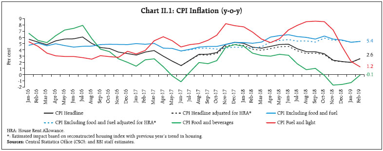 Food prices moved into deflation from October 2018, with a sustained fall in prices of vegetables, fruits and sugar due to robust supplies. In contrast to past trends, milk prices declined abruptly in October coming from high domestic availability. Furthermore, prices of cereals and pulses also saw declines during H2:2018-19 in spite of an increase in minimum support prices (MSPs). Crude oil prices, which were assumed to remain at US$ 80 per barrel at the time of the October MPR, fell sharply to touch a low of US$ 52 per barrel by end-December, before reverting to US$ 68 per barrel by end-March, pulling down inflation in CPI excluding food and fuel. Mirroring this downturn in crude oil prices, domestic LPG prices also collapsed from their recent peak in November. In addition, the trajectory of electricity inflation shifted dramatically downwards since November 2018, pulling down fuel inflation from 8.5 per cent in October to 1.2 per cent in February 2019. In the event, the path of inflation fell below projections by 1.3 percentage points in Q3 and by 2.2 percentage points in Q4 up to February (Chart II.2). 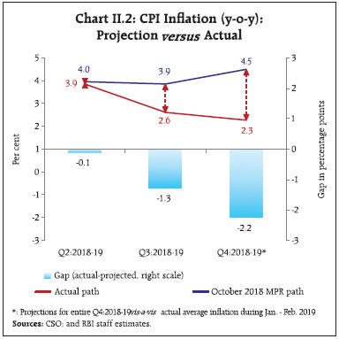 II.1 Consumer Prices The sustained softening in headline inflation during H2:2018-19 reflected initially the combined impact of favourable base effects (October-November) and thereafter a sharp decline in price momentum even when these base effects turned adverse (December-January).2 CPI food, driven down by favourable base effects and a decline in prices, moved into deflation in October 2018, which further deepened in November and persisted till Ferbuary 2019. It was only in February that contraction in food prices got arrested. In the fuel group, inflation moderated sharply on a sustained fall in price momentum. Price momentum in CPI excluding food and fuel, which registered a sharp pick-up in October, moderated thereafter during November-January, with tailwinds from favourable base effects resulting in a moderation of inflation. However, there was an upturn in price momentum in this category in February (Chart II.3). This, along with an upturn in food momentun caused CPI headline momentum to turn positive in February. The distribution of inflation across CPI groups in 2018-19 had striking commonalities with the preceding year, with similar median inflation rates and a persistent negative skewness in both the years emanating from food prices (Chart II.4). Diffusion indices of price changes in CPI items on a seasonally adjusted basis showed moderation during September-January. Much of it was reversed in February; however, more than four-fifths of the CPI basket, comprising both goods and services, experienced price increases, indicating a generalised pick-up in prices in that month (Chart II.5).3 II.2 Drivers of Inflation A historical decomposition of inflation shows that the moderation in inflation in H2:2018-19 was largely the result of favourable supply side shocks - particularly to prices of food and crude oil. Subdued demand pressures opened up a slightly negative output gap, which along with muted wage growth, produced a generalised decline in inflation (Chart II.6a).4 The break-up of overall inflation into goods and services components shows the predominant role of prices of goods in this broad-based downturn (Chart II.6b). These include perishable goods like vegetables and fruits (with a 7-day recall), non-perishable goods like cereals and pulses (with a 30-day recall) in Q3, and imported goods (gold, silver, petrol, diesel, LPG, kerosene, refined vegetables oils, electronic goods, chemical products, metal products, and clothing) in Q4 (up to February) (Chart II.6c).5 Services inflation remained sticky, even as the statistical effects of HRA increases for central government employees dissipated completely. CPI Food Group In terms of weighted contributions, the food and beverages group (weight: 45.9 per cent in CPI) contributed 9.5 per cent to overall inflation during April 2018 - February 2019 as compared with 28.9 per cent for the same period a year ago. Inflation in the food group moved into negative territory from October 2018 and was at (-) 0.1 per cent in February 2019 (Chart II.7a). Four food sub-groups – fruits, vegetables, pulses and sugar with a combined weight of 12.7 per cent in the CPI basket – remained in deflation in February 2019 (Charts II.7 a and b). Within the food group, inflation in respect of cereals (weight of 9.7 per cent in CPI and 21.1 per cent in the food and beverages group) picked up to 1.3 per cent in February 2019 from an intra-year low of 0.8 per cent in January, primarily driven by a modest recovery in rice inflation to (-) 1.9 per cent in February from (-) 2.1 per cent in January as a result of higher production and stocks much above buffer norms. As per the second advance estimates, production of rice was at 115.6 million tonnes in 2018-19, up from the record level of 112.9 million tonnes in 2017-18 (fourth advance estimates). A decomposition of CPI cereals inflation shows a negative contribution of cyclical factors in 2018-19 (Chart II.8). Prices of vegetables, which account for 6.0 per cent of CPI and 13.2 per cent of the food and beverages group, were the principal driver of the unusual food inflation dynamics witnessed during the year; the other key driver was fruits. A sharp fall in prices of vegetables and fruits, combined with a moderation/decline in prices of some protein-rich items (particularly, milk and products, and pulses), oils and fats, and sugar and confectionery kept overall food prices in deflationary zone from October 2018 to February 2019. The easing of food prices in early 2018-19 has, in fact, defied the historical pattern. Also, the rise in food prices during February was, in contrast to past trends, driven largely by a turnaround in fruits prices and recovery in prices of vegetables. 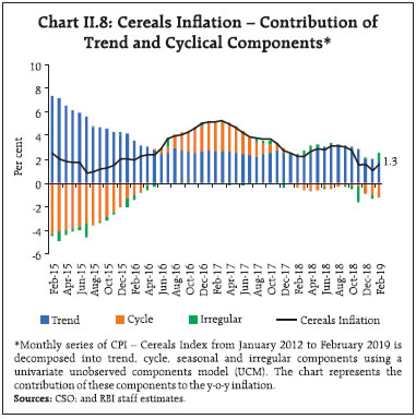 Within vegetables, inflation in respect of onion prices declined from a high of 40.6 per cent in July 2018 to (-) 57.1 per cent in January 2019, followed by some pick-up in February to (-) 49.5 per cent. Gains in kharif production, higher mandi arrivals as well as release of old stocks aided this fall. Tomato prices remained in deflation from March 2018 to January 2019, with negative momentum during August 2018 - February 2019 (barring January), again on account of healthy mandi arrivals and higher production. Anecdotal evidence suggests that the pick-up in tomato prices in January 2019 was largely due to delayed harvesting on account of acute cold conditions following rainfall in Nashik – a major tomato-growing district in Maharashtra, crop damage by fungus in Karnataka and adverse impact on the crop by cyclone Gaja in Tamil Nadu (particularly, in Dindigul, which is a major tomato supplier). However, inflation in respect of potatoes remained in double digits throughout 2018-19 (up to February), despite some moderation since October 2018. Price pressures were visible during March-July 2018 due to lower availability of stocks from cold storages, transport disruptions and protests organised by potato farmers (Chart II.9a). With fresh arrivals entering the market on the back of a bumper winter crop, prices declined during November-February. On the whole, a significantly lower build-up in the cumulative momentum of prices of vegetables in 2018-19 relative to the previous year helped in keeping food inflation low. 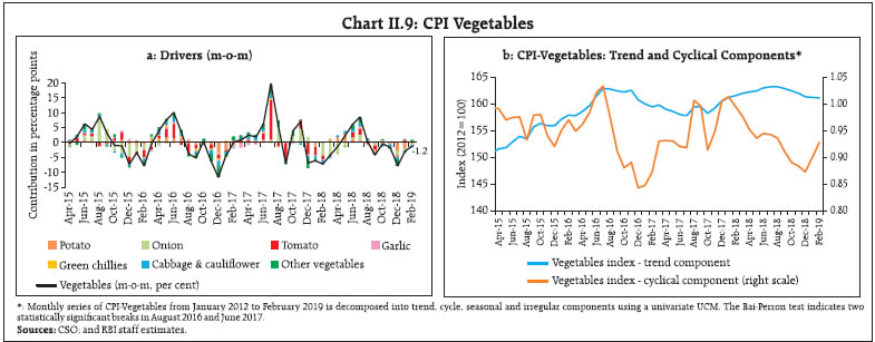 An analysis of prices of vegetables based on sectoral CPI indices suggests that even as month-on-month volatility was higher in urban markets than their rural counterparts, the difference in monthly changes in prices between rural and urban areas was not found to be statistically significant, suggesting that rural-urban price changes were broadly in the same direction.6 A decomposition of CPI-vegetables into trend and cyclical components reveals that a large cyclical downturn till December 2018 was the key mover as the trend component remained more or less flat (Chart II.9b). Some upturn observed since January 2019 in the cyclical component of prices has contributed to a lower rate of decline in prices of vegetables in Q4 (January-February). Prices of fruits (weight of 2.9 per cent in the CPI and 6.3 per cent within the food and beverages group) were another downside surprise during 2018-19. Fruit prices fell in June-July 2018, contrary to past patterns. Strong domestic arrivals of mangoes and bananas, together with higher imports of some fruits (particularly apples and citrus fruits) pulled down domestic prices. Overall, prices of fruits witnessed a sustained decline during June 2018 - January 2019 (except November 2018), contrary to the usual pattern (Chart II.10). While deflation in fruits prices persisted during December 2018 - February 2019, their momentum underwent a sharp upturn in February 2019 in contrast to the average negative momentum of (-) 2.6 per cent in the previous two months. In the case of prices of pulses, deflation persisted on the back of oversupply, although this trend is reversing gradually. Pulses account for 2.4 per cent of the CPI and 5.2 per cent of the food and beverages group. The contribution of pulses to overall inflation was (-) 6.0 per cent during April-February 2018-19 as against (-) 18.9 per cent during April-February 2017-18. With production and procurement of pulses in 2018-19 remaining broadly at the previous year’s level, mandi level prices of some varieties such as arhar and urad have recovered and moved up towards their MSPs in some of the major producing states. Pulses prices have been ruling well below their historical trend for 10 months now (Chart II.11). 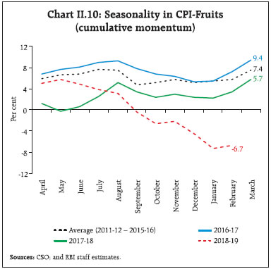 The deflation in prices of the sugar and confectionery sub-group since February 2018 because of excess domestic production, increased open market sales and deflationary movements in global sugar prices, contributed to the subdued food inflation. The increase in the minimum selling prices of sugar by ₹ 2 per kg. to ₹ 31 per kg. by the central government in February 2019 has not yet been reflected in domestic retail prices. Prices of oils and fats remained subdued since September 2018 in line with international edible oils prices. As per the second advance estimates of the Ministry of Agriculture and Farmers’ Welfare, oilseeds production is likely to go up marginally by 0.6 per cent in 2018-19 (over the fourth advance estimates of 2017-18) as the decline in groundnut seeds production is offset by higher production in soybean and mustard seeds. The Government of India has also reduced the import duty on crude palm oil and refined, bleached and deodorised (RBD) palm oil imports from Malaysia and Indonesia, effective January 1, 2019. 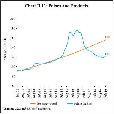 Prices of protein-rich items such as eggs, meat and fish witnessed upside pressure. In the case of eggs, inflation after remaning in negative territory during November 2018 - January 2019, turned positive in February. Meat and fish prices also experienced upside pressures that are typical during the winter months. Inflation in respect of meat and fish was at 5.9 per cent in February, the highest since October 2016, due to higher input prices relating to maize and soybean that constitute animals and poultry feed stock. After reaching an intra-year high of 3.0 per cent in November, inflation in spices eased to 1.8 per cent in February on account of a broad-based decline in prices, reflecting higher expected production of turmeric, dried chillies, dhania and jeera. CPI Fuel Group Fuel and light inflation, which was at 8.5 per cent in October 2018, moderated to 4.5 per cent in December and further to 1.2 per cent in February on account of a fall in prices of LPG along with sustained moderation in electricity, and firewood and chips prices (Chart II.12a). After registering significant price increases between June and November, domestic LPG prices declined abruptly since December, following a collapse in prices in the international market. After the migration of subsidy payments on LPG to bank accounts under the direct benefit transfer scheme, LPG prices in CPI mirror open market prices, which, in turn, track international prices closely (Chart II.12b).  Inflation in electricity, which constitute around one-third of the fuel and light sub-group, moderated to an average of 0.6 per cent in H2:2018-19 (up to February), after hovering around 3 per cent during H1:2018-19. Energy deficit continues to decline despite the stagnation in generation of electricity in January-February 2019 (0.7 per cent y-o-y growth) indicating subdued demand, which is also reflected in low spot prices at the Indian Energy Exchange during this period. Inflation in respect of items of rural consumption such as firewood and chips, which remained sticky and elevated till October, since then declined by 5.4 percentage points to touch 0.6 per cent in February, accentuating the fall in the fuel group inflation. However, administered kerosene prices registered sustained increases as oil marketing companies (OMCs) raised prices in a calibrated manner to phase out subsidy. CPI Excluding Food and Fuel CPI inflation excluding food and fuel saw an uptick in October 2018 which was, however, short-lived as it softened sequentially from 6.2 per cent in October to 5.2 per cent in January 2019 before edging up marginally to 5.4 per cent in February. It is noteworthy though that CPI inflation excluding food and fuel has remained above 5 per cent since December 2017. Excluding volatile items such as petrol, diesel, gold and silver, CPI inflation remained between 5.5-5.8 per cent since October (Chart II.13). Housing, having a weight of 21.3 per cent in CPI excluding food and fuel, was the largest contributor (22 per cent) to inflation in this group, even as the statistical impact of HRA increases of central government employees waned completely by December. The health sub-group, with a weight of 12.5 per cent, contributed around 18 per cent to CPI inflation excluding food and fuel during October-February (Chart II.14). The transport and communication sub-group contributed around 14 per cent – the third highest – to inflation in CPI excluding food and fuel, with its contribution much below its weight of 18.2 per cent due to a sharp decline in petrol and diesel prices since November (Chart II.15a). The wedge between international and domestic prices remains considerable due to the asymmetric pass-through of international crude oil prices to domestic prices since 2014 (Chart II.15b). Among other sub-groups, education (weight of 9.4 per cent in CPI excluding food and fuel) contributed around 13 per cent to CPI inflation excluding food and fuel in H2 (up to February) due to a pick-up in inflation in tuition fee, books and journals. In contrast, a sharp moderation in clothing and footwear inflation from October 2018 pulled down its contribution to inflation in CPI excluding food and fuel to 8 per cent, well below its weight of 13.8 per cent in the group (Chart II.14). Disaggregation of CPI inflation excluding food, fuel, petrol and diesel into goods and services shows that goods inflation moved in a narrow range of 4.9-5.1 per cent during H2:2018-19 (up to February), while services inflation persisted at elevated levels – 6.0-6.5 per cent. Goods inflation picked up in Q3 across commodity groups – particularly medicines, household goods, and items of personal care and effects – offset somewhat by a sharp moderation in clothing and footwear sub-group inflation (Chart II.16a). Sticky and elevated services inflation in Q3 was primarily on account of a rise in transportation fares, education expenses and household services, which more than offset the significant moderation in housing inflation on waning HRA effects. During January-February 2019, services inflation moderated somewhat from 6.2 per cent to 6.0 per cent as transportation services inflation eased, reflecting the lagged impact of lower fuel prices and also on account of some moderation in inflation in respect of housing, education and ‘personal care and effects’ services (Chart II.16b). 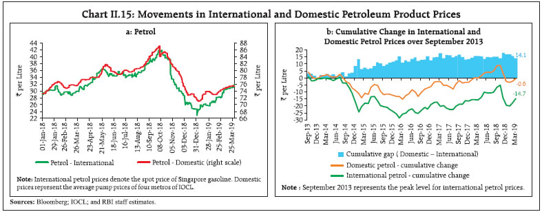 Other Measures of Inflation Measures of inflation other than the CPI showed mixed movements since the October MPR. Inflation measured by sectoral CPIs – for industrial workers (CPI-IW), agricultural labourers (CPI-AL) and rural labourers (CPI-RL) – edged up during November to February 2019. First, food inflation in all the three sectoral CPIs was higher relative to all India CPI. Second, fuel inflation remained range bound and did not collapse in sectoral CPIs. The housing index in the CPI-IW is revised once in six months, i.e., in January and July every year. Following the increase in HRA under the 7th central pay commission (CPC), the housing index in the CPI-IW increased by 8.8 per cent and 15.9 per cent in January and July 2018, respectively, and further by 8.8 per cent in January 2019. CPI-IW inflation shot up to 7.0 per cent in February from 5.2 per cent in December, pulled up by the January 2019 increase in its housing index. 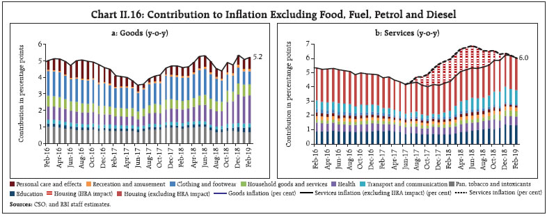 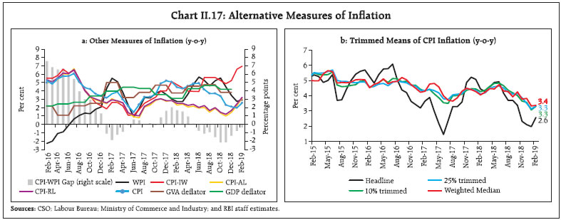 In contrast, wholesale price index (WPI) inflation fell from its October 2018 peak of 5.5 per cent to 2.8-2.9 per cent in January-February. The sequential decline in WPI inflation was led by a significant fall in inflation in respect of crude petroleum, mineral oils and basic metals, tracking international commodity prices. GDP and GVA deflators also edged down in Q3 in line with WPI inflation (Chart II.17a). Volatile prices of items such as food, fuel and precious metals impart high dispersion, asymmetry and non-normality to the distribution of inflation. To gauge underlying inflation dynamics, one way is to remove high positive as well as negative skewness and chronic fat tails in the inflation distribution by trimming the tails. In addition to exclusion based measures discussed earlier, trimmed means of CPI have softened sequentially over the last six months (Chart II.17b). Inflation measures, which remove the volatile components and represent the durable component of inflation, can be evaluated against desirable properties of 'core' inflation. An analysis of eleven inflation measures suggests that none of the exclusion-based measures satisfied all the properties of 'core' inflation. However, two statistical measures, viz., trimmed means (5 per cent and 10 per cent) satisfied all the properties of a core measure, other than the ease of communication (Box II.1). II.3 Costs Underlying cost conditions have largely co-moved with WPI inflation. Industrial and farm costs captured under the WPI picked up in Q1:2018-19 and remained elevated till November 2018, after which they moderated considerably (Chart II.18). Global crude oil prices declined sharply during November-December 2018 from their peak levels in October 2018 before edging up in January and February 2019. This decline got passed on to prices of inputs such as high-speed diesel, aviation turbine fuel, naphtha, bitumen, furnace oil and petroleum coke, pulling down domestic farm and non-farm input costs. Though some of the petroleum product prices increased in February 2019, reflecting the increase in crude oil prices, industrial input costs continued to decelerate due to a sharp decline in mineral prices. Among other industrial raw materials, domestic coal inflation eased during January-February 2019 largely due to favourable base effects. Inflation in paper and pulp prices edged up in Q3:2018-19 due to rising production costs and global prices. Inflation in fibres picked up in Q2 and Q3 after being in negative territory in Q1. However, it has moderated since December 2018 due to softening prices of raw cotton on account of weak demand from domestic yarn mills and excess stocks in overseas markets. Box II.1: Core Inflation Measures in India – An Empirical Evaluation Movements in headline inflation are influenced by its trend and by changes of a temporary nature. While the transitory elements largely reflect supply shocks, the trend component responds to changes in aggregate demand conditions and expectations. This persistent component of inflation, often referred to as core or underlying inflation, provides an important guide to the future path of headline inflation. Hence, a core inflation measure is often used by monetary authorities as an input for the conduct of monetary policy. Two commonly used approaches to measure core inflation are (i) exclusion-based measures i.e., excluding some highly volatile elements from the headline such as food and fuel; and (ii) statistical measures such as median or trimmed mean. There are some properties that a core inflation measure should satisfy: credibility: a measure of core inflation should be timely, credible (verifiable by agents independent of the central bank) and easily understood by the public. mean and standard deviation: a core inflation measure should have the same mean as the headline, but lower standard deviation. reversion: an appropriate measure of core inflation is the one to which headline reverts; hence, core inflation measure can be a good predictor of future inflation. core inflation causes headline, but headline does not cause core: core and headline need to be cointegrated with a unitary coefficient (termed as unbiasedness). In other words, core is strongly exogenous (with respect to headline), but headline is not. correlation with past monetary policy: monetary policy over a longer horizon is more likely to be correlated with durable or core CPI inflation. A total of eleven CPI core measures for India were considered out of which six were exclusion-based measures, viz.: (i) excluding food and fuel; (ii) excluding food, petrol and diesel; (iii) excluding food, fuel, petrol and diesel; (iv) excluding food, petrol, diesel, gold and silver; (v) excluding food, fuel, petrol, diesel, gold and silver; and (vi) excluding food, fuel, petrol, diesel, gold, silver and housing. Five statistical measures considered are: (i) trimmed mean (5 per cent); (ii) trimmed mean (10 per cent); (iii) trimmed mean (20 per cent); (iv) median; and (v) reweighting the index based on historical standard deviation. Based on data from January 2012 to February 2019, headline inflation is treading below the lower range of the band constructed by using all the eleven core measures (Chart II.1.1). For the full period, all exclusion-based measures satisfied all the properties other than (i) being a robust future inflation predictor; and (ii) correlation with past monetary policy (Table II.1.1). However, if the sample period is truncated to mid-July 2018, the property of being an efficient future inflation predictor is also satisfied. This suggests that the recent unusual period of low and persistent food inflation has impaired the predictive properties of exclusion-based measures. Also, the property of correlation with the past monetary policy was not satisfied by any exclusion-based measure. This was possibly due to the reason that it was only in January 2014 that the RBI adopted CPI as the headline inflation measure. It is also significant that often inflation in WPI and sectoral CPIs registered wide divergence. The trimmed mean measures (5 per cent and 10 per cent) satisfied all the desirable properties in the full sample. However, statistical measures of core inflation are not easy to communicate. | Table II.1.1: Properties of CPI Core Inflation Measures | | | Properties → | Ease of Communication | Equality of means | Less variance | Future inflation predictor | Co integrated | Unbiasedness | Attraction condition | Correlation with past monetary policy | | Measures↓ | | | | (1) | (2a) | (2b) | (3) | (4a) | (4b) | (4c) | (5) | | 1. | Excluding Food and Fuel | √ | √ | √ | x | √ | √ | √ | x | | 2. | Excluding Food, Petrol and Diesel | √ | √ | √ | x | √ | √ | √ | x | | 3. | Excluding Food, Fuel, Petrol and Diesel | √ | √ | √ | x | √ | √ | √ | x | | 4. | Excluding Food, Petrol, Diesel, Gold and Silver | √ | √ | √ | x | √ | √ | √ | x | | 5. | Excluding Food, Fuel, Petrol, Diesel, Gold and Silver | √ | √ | √ | x | √ | √ | √ | x | | 6. | Excluding Food, Fuel, Petrol, Diesel, Gold, Silver and Housing | √ | √ | √ | x | √ | √ | √ | x | | 7. | Trimmed Mean (5 per cent) | x | √ | √ | √ | √ | √ | √ | √ | | 8. | Trimmed Mean (10 per cent) | x | √ | √ | √ | √ | √ | √ | √ | | 9. | Trimmed Mean (20 per cent) | x | √ | √ | √ | √ | x | x | x | | 10. | Median | x | √ | √ | x | √ | √ | x | x | | 11. | Historical Standard Deviation | x | √ | √ | √ | √ | √ | √ | √ | | Note: √: property satisfied; x: property not satisfied. | References: Das, A., J. John and S. Singh (2009), “Measuring Core Inflation in India”, Indian Economic Review, July December. Das, P. and A.T. George (2017), “Comparison of Consumer and Wholesale Prices Indices in India: An Analysis of Properties and Sources of Divergence”, RBI Working Paper Number 5/2017, May. Raj, J. and S. Misra (2011), “Measures of Core Inflation in India – An Empirical Evaluation”, Reserve Bank of India Occasional Papers, Vol. 32, No. 3, Winter, pp 37-66. Raj, J., S. Misra, A. T. George, and J. John (2019) “Measures of Core Inflation in India – An Empirical Evaluation using CPI data”, mimeo. | In the case of farm sector inputs, inflation in respect of fertilisers and pesticides increased in Q2:2018-19 and Q3, while fodder inflation turned positive in January 2019 and edged up further in February, after remaining negative for 16 consecutive months. Fertiliser prices rose in line with the increase in global prices of phosphate and potash, while prices of pesticides were impacted by an uptick in global crude oil prices. Inflation in respect of agricultural machinery and implements prices picked up in Q2 and Q3, but eased marginally in Q4 (up to February). Inflation in electricity, which carries a high weight in both industrial and farm inputs, remained elevated and volatile during 2018-19. Nominal growth in rural wages for both agricultural and non-agricultural labourers remained muted in Q3:2018-19, reflecting the lagged impact of moderate rural inflation and low food prices (Chart II.19). Pressures from staff costs in the organised sector have been range-bound. Per employee staff costs in the manufacturing sector, which declined in the first two quarters of 2018-19, edged up in Q3:2018-19. In the services sector, per employee staff cost growth increased by 2.2 per cent in Q3:2018-19 as compared with 0.1 per cent in the previous quarter (Chart II.20a). Unit labour costs for companies in the manufacturing sector ticked up in Q3:2018-19.7 In the services sector, unit labour costs flattened in Q1:2018-19 but edged up in the next two quarters. The growth in staff costs outpaced the growth in value of production in both the manufacturing and services sectors in Q3 (Chart II.20b). Easing of commodity prices, particularly of crude petroleum, mineral oils and metals, was also reflected in the moderation in input costs of manufacturing firms covered in the Reserve Bank’s industrial outlook survey. Fewer firms assessed an increase in cost of raw materials in Q4:2018-19 than in the last two quarters and the decline is expected to continue in Q1:2019-20. Firms passed the cost benefit on to their selling prices in Q4 and expected moderation in selling prices in the first quarter of 2019-20. Firms polled in the manufacturing purchasing managers’ index (PMI) also reported a decline in input costs and selling prices for the second consecutive quarter in Q4:2018-19. However, the rate of decline in selling prices was lower than that of input costs. In contrast, input cost inflation reported by firms in the services sector in the PMI was marginally higher in Q4:2018-19 than in the previous quarter. The increase in prices charged by these firms remained subdued in Q3 and Q4. II.4 Conclusion Headline CPI inflation movements were characterised by unprecedented and, to a large extent, unanticipated collapse in inflation in food and fuel, which together constitute around 53 per cent of the CPI basket. Inflation in the remaining 47 per cent of the CPI basket, comprising items excluding food and fuel, also moderated somewhat in Q4:2018-19, notwithstanding the fact that the levels were still elevated. Inflation outcomes going forward will largely be shaped by movements in food inflation. Record agricultural production, high stocks of food grains and effective supply management measures by the government have kept food inflation in check in recent years. Should the monsoon turn out to be normal, food inflation is likely to remain contained in 2019-20. 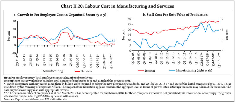 The fuel inflation trajectory is also likely to be shaped by movements in international energy prices. Should the domestic economic activity slow down further, it will reduce the risk of sudden demand side pressures impinging on CPI inflation excluding food and fuel. Inflation expectations of both households and producers have softened, and professional forecasters also expect inflationary pressures to remain contained. There are also some upside risks to inflation, which emanate largely from oil – from a further tightening of crude supplies due to continuing production cuts by the Organisation of the Petroleum Exporting Countries (OPEC), Iran sanctions and Venezuela turmoil, as also from the demand side if trade tensions are resolved suitably. Fiscal slippage at the centre and/or state levels, if any, represents another medium-term risk to the inflation trajectory through higher aggregate demand pressures and crowding out of private investment. Given its past volatility, food inflation reversal poses another significant upside risk, especially in view of reports of some probability of El Niño this year and its implications for monsoon. On the whole, though inflation is likely to edge up from current levels, it is projected to remain within the Reserve Bank’s target of 4 per cent during 2019-20. _____________________________________________________________________________
III. Demand and Output Economic activity slowed down in Q2 led mainly by a large drag from net exports, which became entrenched in Q3 due to deceleration in public spending and private consumption. On the supply side, agriculture and allied activities moderated characterised by a modest growth in kharif and horticulture production. Industrial growth also decelerated led by a slowdown in manufacturing activity. However, services sector activity remained resilient, supported primarily by construction, financial services, and public administration and defence. Domestic economic activity lost pace in Q2 and Q3, with coincident indicators suggesting a sharper deceleration in Q4. Aggregate demand weakened in Q2 by a large drag from net exports, followed by a slowdown in consumption, both private and government, in Q3. By contrast, gross fixed capital formation (GFCF) growth remained in double digits for the fifth consecutive quarter in Q3. On the supply side, agriculture and allied activities slowed down in Q2 and Q3, with increases in kharif and horticulture production turning out to be modest relative to last year’s record. Higher input costs, particularly stemming from crude oil prices, and weaker pricing power, impacted profit margins of firms and restrained manufacturing. In the services sector, activity picked up on the back of growth of financial services and construction activity which was supported by public infrastructure spending. However, trade, hotels, transport, and communication services lost momentum in Q2 and remained flat in Q3. III.1 Aggregate Demand The growth in aggregate demand, measured by y-o-y changes in real GDP at market prices, moderated to 6.5 per cent in H2:2018-19 from 7.5 per cent in H1 and 7.9 per cent a year ago. The slowdown was caused by lower though still healthy growth of 9.1 per cent in GFCF in H2 as compared with 10.9 per cent in H1. Private consumption was sustained by higher spending on durable goods and services, while government spending accelerated in H2 on account of higher spending by states. These disparate movements were reflected in shifts in weighted contributions of the components to GDP growth (Chart III.1a and Table III.1). Overall, however, the moderation in GDP growth in H2 can be attributed to adverse base effects even as momentum, measured by the q-o-q seasonally adjusted annualised growth rate (SAAR), accelerated during the same period (Chart III.1b). 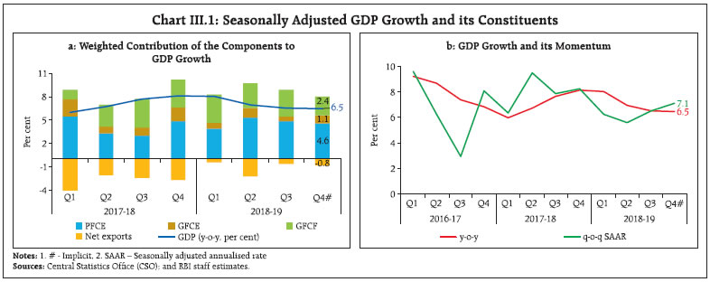 | Table III.1: Real GDP Growth | | (y-o-y, per cent) | | Item | 2017-18 (FRE) | 2018-19 (SAE) | Weighted Contribution* | 2017-18 (FRE) | 2018-19 (SAE) | | 2017-18 | 2018-19 | Q1 | Q2 | Q3 | Q4 | Q1 | Q2 | Q3 | Q4# | | Private final consumption expenditure | 7.4 | 8.3 | 4.2 | 4.7 | 10.1 | 6.0 | 5.0 | 8.8 | 6.9 | 9.8 | 8.4 | 8.1 | | Government final consumption expenditure | 15.0 | 8.9 | 1.5 | 0.9 | 21.9 | 7.6 | 10.8 | 21.1 | 6.5 | 10.8 | 6.5 | 11.6 | | Gross fixed capital formation | 9.3 | 10.0 | 2.9 | 3.1 | 3.9 | 9.3 | 12.2 | 11.8 | 11.7 | 10.2 | 10.6 | 7.7 | | Exports | 4.7 | 13.4 | 1.0 | 2.7 | 4.9 | 5.8 | 5.3 | 2.8 | 11.2 | 13.9 | 14.6 | 14.0 | | Imports | 17.6 | 15.7 | 3.8 | 3.7 | 23.9 | 15.0 | 15.8 | 16.2 | 10.8 | 21.4 | 14.7 | 16.1 | | GDP at market prices | 7.2 | 7.0 | 7.2 | 7.0 | 6.0 | 6.8 | 7.7 | 8.1 | 8.0 | 7.0 | 6.6 | 6.5 | FRE: First Revised Estimates; SAE: Second Advance Estimates; #: Implicit growth
*: Component-wise contributions to growth do not add up to GDP growth in the table because change in stocks, valuables and statistical discrepancies are not included.
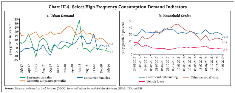
Source: CSO. | GDP Projections versus Actual Outcomes The October 2018 Monetary Policy Report (MPR) projected GDP growth at 7.4 per cent in Q2, 7.3 per cent in Q3 and 7.1 per cent in Q4 of 2018-19, with risks evenly balanced around this baseline path (Chart III.2). Actual outcomes in terms of the second advance estimates (SAE) of the CSO released on February 28, 2019 undershot these projections by 40 and 70 basis points in Q2 and Q3, respectively. The downward surprise in Q2 stemmed from a stronger than anticipated drag from net exports, mainly due to a sharp acceleration in the import bill on the back of a surge in international crude prices. In Q3, projection errors emanated mainly from a sharper than expected slowdown in government consumption as revenue expenditure growth of central government nosedived. In the event, overall GDP growth for 2018-19 at 7.0 per cent in the SAE (February 28, 2019) turned out to be lower than the projection of 7.4 per cent in the October MPR. III.1.1 Private Final Consumption Expenditure Private final consumption expenditure (PFCE) remained the mainstay of aggregate demand, with its share rising to 57.9 per cent in H2:2018-19 from 57.0 per cent a year ago. Its resilience drew on a combination of factors, viz., low retail inflation that expanded disposable incomes, the significant softening of global crude oil prices and resulting economies in energy outgoes, expansion of public spending in rural areas, and strong growth in personal and consumer loans, notwithstanding a slowdown in agriculture and labour-intensive exports, which could have adversely impacted rural consumption (Chart III.3). High frequency indicators of urban consumption have, however, moderated significantly in Q4:2018-19. Growth in domestic air passenger traffic continued to decelerate (Chart III.4.a). Passenger car sales have been contracting since July 2018, inter alia, due to volatility in fuel prices and mandated long-term upfront insurance premium payments. Going forward into 2019-20, urban consumption may get some support from the spending uptick associated with general elections, increase in disposable incomes due to a relaxation in income tax, and prospects of sustained growth in personal bank loans (Chart III.4b). 
 Among the indicators of rural demand, sales of motorcycles remained in contraction zone. Tractor sales also sharply decelerated in recent months possibly due to weak rabi sowing and subdued farm prices. The production of consumer non-durables remained lacklustre (Chart III.5). Robust growth in construction activity in H2:2018-19 – an employment-intensive sector – should augur well for rural incomes and demand. Rural demand may also get some support from policy measures announced recently, viz., implementation of PM Kisan Samman Yojana (PMKSY), direct income transfer schemes, farm loan waivers by many states, and the government’s continued thrust on rural infrastructure spending. III.1.2 Gross Fixed Capital Formation Growth in gross fixed capital formation (GFCF) has remained in double digits since Q3:2017-18, though it is likely to slow down in Q4 as some of the key indicators of investment demand, viz., capital goods production and imports have decelerated. The share of GFCF in GDP improved to 32.3 per cent in 2018-19 from 31.4 per cent a year ago, indicating an incipient strengthening of investment demand. The pick-up in fixed investment was supported by higher construction activity, led by the government’s drive to boost spending on the road sector and affordable housing. The performance of software firms – a proxy for investment in intellectual property products – has also been healthy as reflected in their latest financial results. The ongoing resolution of distressed assets of non-financial corporates under the Insolvency and Bankruptcy Code (IBC) process is expected to unlock resources for investment activity. However, growth of capital goods imports – another proxy for investment demand – contracted in February 2019 (Chart III.6a). Production of capital goods also either contracted or remained tepid from November 2018 to January 2019. Seasonally adjusted capacity utilisation (CU-SA), however, crossed its long-term average in Q3:2018-19, which could encourage fresh capacity addition and capex (Chart III.6b). Sustained growth in housing loans disbursed by scheduled commercial banks (SCBs) also bodes well for investment in dwellings. The pick-up in investment demand was financed by non-food bank credit and inflows of foreign direct investment (FDI) (see Chart III.7; and Chapter IV for details). Overall, there has been an improvement in the flow of resources from the financial sector to the non-financial corporate sector, which should support the private capex cycle.
Half-yearly financial statements of listed non-government non-financial (NGNF) companies suggest a decline in the capex ratio in H1:2018-19 over H2:2017-18 across manufacturing industries, and notably, in cement and cement products, iron and steel, pharmaceuticals and medicines, and textiles (Chart III.8).1 The decline in the capex ratio for iron and steel was on account of overall deleveraging that was underway in the sector; on the other hand, the ratio for petroleum product firms improved significantly. With debt levels declining in some sectors and the resolution of stressed assets under the IBC, the capex ratio could improve, going forward. 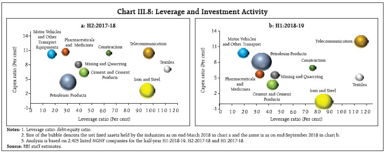 Notwithstanding recent improvements, the investment rate has declined significantly since 2012-13, mirroring the decline in the saving rate over these years (Chart III.9a). The savings rate of the household sector, which is a net supplier of funds to the economy, declined from 23.6 per cent of GDP in 2011-12 to 17.2 per cent in 2017-18. While the private corporate sector financed its investment predominantly through its own saving, the public sector continues to rely heavily on households for resources (Chart III.9b). III.1.3 Government Expenditure Government final consumption expenditure (GFCE) supported aggregate demand in H2:2018-19, especially in Q4. GFCE is likely to augment aggregate demand in 2019-20 too, in view of higher outgoes in the Interim Union Budget on agriculture and various income support schemes. Revenue expenditure growth budgeted for 2019-20 is also higher than in 2018-19 (RE) (Table III.2). | Table III.2: Key Fiscal Indicators – Central Government Finances | | Indicator | Per cent to GDP | | 2018-19 (BE) | 2018-19 (RE) | 2019-20 (BE) | | 1. Revenue Receipts | 9.1 | 9.1 | 9.4 | | a. Tax Revenue (Net) | 7.8 | 7.8 | 8.1 | | b. Non-Tax Revenue | 1.3 | 1.3 | 1.3 | | 2. Non-Debt Capital Receipts | 0.5 | 0.5 | 0.5 | | 3. Revenue Expenditure | 11.2 | 11.2 | 11.7 | | 4. Capital Expenditure | 1.6 | 1.7 | 1.6 | | 5. Total Expenditure | 12.8 | 12.9 | 13.3 | | 6. Gross Fiscal Deficit | 3.3 | 3.4 | 3.4 | | 7. Revenue Deficit | 2.2 | 2.2 | 2.2 | | 8. Primary Deficit | 0.3 | 0.2 | 0.2 | Note: BE: Budget Estimates. RE: Revised Estimates.
Source: Union Budget, 2019-20. | During 2018-19 (April-February), the fiscal position of the central government deteriorated mainly because of muted growth in indirect tax revenues (Chart III.10a and b). Revenue expenditure (87.5 per cent of total expenditure) evolved broadly as budgeted [growth of 12.5 per cent till February 2019 vis-à-vis 13.9 per cent in revised estimates (RE)], though payments of food and fertiliser subsidies were higher than a year ago. Outgoes on account of major subsidies in 2018-19 are estimated to have remained unchanged in the revised estimates (RE) vis-à-vis the budget estimates (BE) of 1.4 per cent of GDP. While the share of petroleum subsidies is expected to rise in 2019-20, food subsidies will continue to dominate the overall subsidy bill (0.9 per cent of GDP). Although capital expenditure has a larger fiscal multiplier, relative to revenue expenditure, by crowding in private investment, the share of capital expenditure in total expenditure has remained stagnant at around 12-13 per cent in recent years (Box III.1). 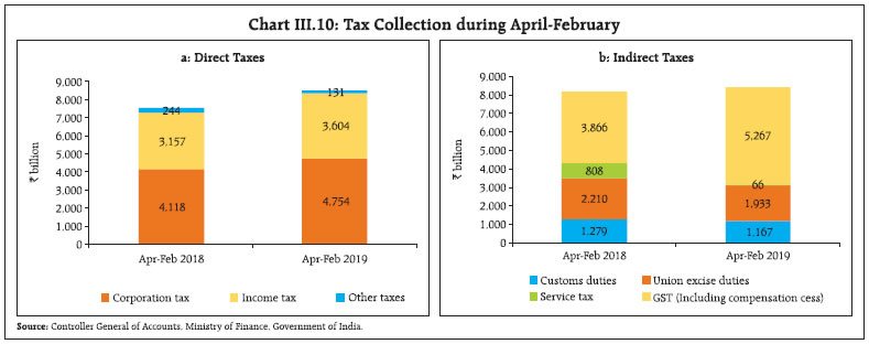 Gross tax collections fell short of the budget target in 2018-19 (RE) largely due to a shortfall in goods and services tax (GST) collections by ₹1 trillion, though corporate tax and customs duty collections surpassed the budget targets. GST revenues at ₹5.3 trillion during April-February 2018-19 constituted 81.5 per cent of RE. Indirect tax growth (April-February 2018-19) remained distinctly lower at 3.3 per cent than 14.3 per cent (RE), while direct tax growth remained modest at 12.9 per cent as against 19.8 per cent in 2018-19 (RE). Consequently, the Centre’s fiscal deficit was 34.2 per cent more than the revised GFD target at the end of February 2019. Accordingly, there was a cutback in capital expenditure, which contracted by 7.9 per cent in April-February 2018-19 as against the growth of 20.3 per cent envisaged in the RE, in order to contain the GFD. Box III.1: Estimable Fiscal Multipliers for India Fiscal policy acts as an instrument of economic stabilisation by influencing aggregate demand and smoothing it over the business cycle. In the process, changes in government spending and taxation can have a significant impact on underlying economic activity. At the height of the global financial crisis (GFC), fiscal stimulus was used widely to prevent national economies from sliding into a depression; after the crisis, however, the withdrawal of stimulus became the centre of an intense and agitated debate on “growth versus austerity”. In this context, an accurate assessment of the fiscal policy-growth relationship assumes importance for the appropriate setting of macroeconomic policy. Fiscal multiplier, defined as a ratio of a change in output to an exogenous change in a fiscal variable (viz., government expenditure/taxation or both), measures the short-term impact of discretionary fiscal policy on output. For policymakers who employ fiscal multipliers, errors in their estimation can have serious policy consequences. For instance, underestimation of fiscal multipliers in the GFC appears to have contributed significantly to growth forecast errors (Blanchard and Leigh, 2013), making countries to set unachievable fiscal targets along with errors on the quantum of adjustments required to meet growth forecasts (Eyraud and Weber, 2013), thereby undermining the credibility of fiscal programmes (Batini et al., 2014). Fiscal multipliers are not always widely used in operational work as their estimation is fraught with difficulties. In particular, isolating the direct effect of fiscal measures on GDP is challenging in view of the problem of “endogeneity” – government expenditure and taxation are “automatic stabilisers” which respond inevitably to the business cycle but can also be used as counter-cyclical instruments, i.e., reducing taxes and increasing spending to stimulate aggregate demand when the output gap is negative. Therefore, extracting exogenous components from observed fiscal outcomes is problematic. Moreover, fiscal multipliers provide little guidance about medium to long-term effects and fiscal sustainability. Consequently, there is little consensus on the appropriate methodology and the desirable size of multipliers. In the literature, fiscal multipliers are often estimated by using Dynamic Stochastic General Equilibrium (DSGE) models, Structural Vector Auto Regressions (SVAR) or Structural Econometric Macromodels (SEM). Although DSGE models are well-grounded in economic theory, they have limited practitioner utility since they do not seem to fit the data well. By contrast, SVAR models only explore historical interactions among a group of economic variables and are considered atheoretic. In this context, SEM – which draw on elements from both DSGE and SVAR models – are considered more useful for policy analysis (Wren-Lewis, 2018). Accordingly, fiscal multipliers for India are estimated in a SEM framework, which follows the schematic representation of causal interlinkages as presented in Chart III.1.12. Briefly, fiscal deficits of central and state governments are disaggregated into various budgetary spending heads in the capital and revenue accounts, shocks to which can be explored through the propagation mechanism of transmission channels. A revenue expenditure shock3 increases private consumption, thereby boosting aggregate demand (measured by the output gap) and output. At the same time, the consequential cutback in capital expenditure in order to adhere to fiscal targets will adversely impact investment demand and, in turn, output. The revenue expenditure shock also increases the fiscal deficit, leading to deviations from the long-term sustainable level of debt. These changes impact the exchange rate through country risk premium and, in turn, inflation. Aggregate demand and inflation condition the short-term interest rate via a monetary policy rule which, in turn, affects long-term interest rates and, hence, the fiscal deficit through interest payments. The monetary policy impulse also impacts aggregate demand, output, exchange rate, and hence, inflation. The rest of the world interacts with domestic variables through various channels viz., global demand conditions impacting India’s exports; US bond yields; US inflation developments; and movements in global crude prices. Coefficients of the simultaneous equation model are estimated from annual data spanning 1980-81 to 2017-18 by employing Bayesian techniques; in particular, unobserved parameters are treated as jointly distributed random variables and are estimated by using subjective and/or non-sample prior information combined with the likelihood function (sample probability distribution) to form a posterior density of the parameters (Table III.1.1). This also overcomes the effects of a small sample bias. 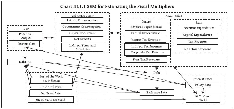 In the Indian context, it is important to note that revenue expenditure multipliers for the central and state governments are less than unity. If revenue expenditure is increased by one rupee, government final consumption expenditure also increases by one rupee, which increases the output by the same amount, provided capital expenditure remains unchanged. This also induces a positive impact on consumption demand. Empirical estimates, however, suggest that there exists a negative relationship between revenue and capital expenditure, given the budget constraint. Consequently, an increase in revenue expenditure by the central and state governments reduces capital expenditure which, in turn, impacts private investment negatively, offsetting the positive effects emanating from the consumption channel and eventually increasing output only by 45 paise and 82 paise, respectively. In contrast, the capital expenditure multiplier is well above unity for both the central and state governments: 3.25 for the central government and 2.0 for state governments. This indicates that an increase in capital expenditure by the central and state governments by one rupee each crowds in private investment, induces a more than proportionate increase in investment in the economy, and leads to an increase in output by 3.25 rupees and 2.0 rupees, respectively. | Table III.1.1: Estimated Fiscal Multipliers | | Sr. No. | Variable | Peak Multiplier | | 1. | Revenue Expenditure
(Central Government) | 0.45 | | 2. | Revenue Expenditure
(State Governments) | 0.82 | | 3. | Capital Expenditure
(Central Government) | 3.25 | | 4. | Capital Expenditure
(State Governments) | 2.00 | | Note: A value of ‘x’ for multiplier implies that an increase in expenditure of the government by ₹1 would raise the GDP by ₹‘x’. | References: Batini, N., Eyraud, L., Forni, L. and Weber, A., 2014. Fiscal multipliers: Size, determinants, and use in macroeconomic projections (No. 14). International Monetary Fund. Blanchard, O.J. and Leigh, D., 2013. Growth forecast errors and fiscal multipliers. American Economic Review, 103(3), pp.117-20. Eyraud, L. and Weber, A., 2013. The challenge of debt reduction during fiscal consolidation (No. -13 67). International Monetary Fund. Ghate, C., Gopalakrishnan, P. and Tarafdar, S., 2016. Fiscal policy in an emerging market business cycle model. The Journal of Economic Asymmetries, 14, pp.52-77. Patra, M.D., Mitra, P., Bhattacharyya, I., Misra, S., Behera, S.R., John, J., Singh, K. and Mate, K., (2019), Estimable Fiscal Multipliers for India, Mimeo. Wren-Lewis, S., 2018. Ending the microfoundations hegemony. Oxford Review of Economic Policy, 34(1-2), pp.55-69. | In the Interim Budget (2019-20), the Centre’s GFD was revised upward to 3.4 per cent of the GDP in 2018-19 (RE) from 3.3 per cent in BE; the target of 3.0 per cent of the GDP has been retained for 2020-21. The deviation in the GFD for 2018-19 was caused mainly by a large shortfall in GST collections and extension of direct income support to farmers. Against the backdrop of heightened pressure on state finances from 2015-16 to 2017-18 due to factors such as the Ujwal DISCOM Assurance Yojana (UDAY), farm loan waivers, pay revisions and decline in revenue collections, the consolidated GFD of 29 states was budgeted at 2.6 per cent of GDP in 2018-19. As on date, 28 states have presented vote-on-account/full budgets for 2019-20. From the consolidated position of 25 states that is available, the consolidated GFD stands revised to 2.9 per cent of GDP for 2018-19 (Table III.3). Out of 15 states, which have recorded slippages, some states have introduced either alternative farm support schemes (Andhra Pradesh and West Bengal) or farm loan waivers (Chhattisgarh, Madhya Pradesh, and Rajasthan). For 2019-20, states have budgeted for a consolidation with the GFD-GDP ratio at 2.5 per cent. Turning to financing, the borrowing programme of the Centre for H1:2018-19 was conducted as per the planned issuance schedule. The government decided to borrow less in H2:2018-19 which led to revision of market borrowing programme for 2018-19 from ₹6,055 billion to ₹5,710 billion (about 3 per cent lower than last year). Thus, the central government completed its revised borrowings as on March 22, 2019 (Table III.4). A strategy of debt consolidation was undertaken through switches to the extent of ₹281 billion during 2018-19. States completed their gross borrowings by March 26, 2019 amounting to ₹4,783 billion. | Table III.3: State Budgets 2019-20 - Key Fiscal Indicators* | | (Per cent to GDP) | | Item | 2017-18 | 2018-19 BE | 2018-19 RE | 2019-20 BE | | Revenue Deficit | 0.2 | -0.1 | 0.1 | 0.0 | | Gross Fiscal Deficit | 2.5 | 2.6 | 2.9 | 2.5 | *: While 2017-18 includes 24 states, remaining years include 25 states.
‘-’: indicates surplus.
Source: Budget documents of state governments. |
| Table III.4: Government Market Borrowings | | (₹ billion) | | Item | 2016-17 | 2017-18 | 2018-19 | | | Centre | States | Total | Centre | States | Total | Centre | States | Total | | Net Borrowings | 4,082 | 3,426 | 7,508 | 4,484 | 3,403 | 7,887 | 4,227 | 3,486 | 7,713 | | Gross Borrowings | 5,820 | 3,820 | 9,640 | 5,880 | 4,191 | 10,071 | 5,710 | 4,783 | 10,493 | | Sources: Government of India; and RBI staff estimates. | III.1.4 External Demand Net exports continued to act as a drag on aggregate demand in H2:2018-19 with growth in imports outpacing exports (Charts III.11a and 11b). Against the backdrop of slowing global trade and commerce-inhibiting trade tensions, India’s merchandise exports (y-o-y) moderated during Q2 and Q3 of 2018-19 relative to Q1 (Chart III.12a). During Q2, the slowdown in exports was accentuated by a decline in shipments of readymade garments, rice and marine products; in Q3, exports growth was pulled down by gems & jewellery, engineering goods, and meat, dairy & poultry. 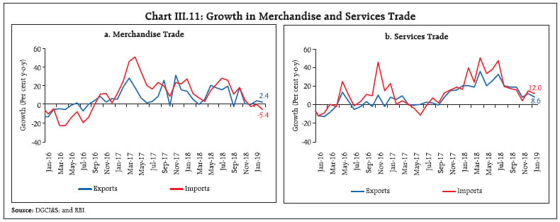 An important feature of India’s export basket in recent years has been a shift away from primary and traditional low value-added exports to higher value-added manufacturing and technology-driven items. This shift has imparted a measure of resilience to export demand in a hostile international trading environment. A comparison of key items of exports between 2011-12 and 2018-19 (April-February) reveals that there has been a significant increase in the shares of chemical and related products and engineering goods (Chart III.13). Going forward, policy initiatives such as hikes in the interest equalisation rates for micro, small and medium enterprises (MSME) exports from 3 per cent to 5 per cent as well as measures announced in the Agriculture Export Policy, 2018 are likely to provide a fillip to exports. After registering a five-quarter high in Q2:2018-19, merchandise import growth decelerated sharply in Q3, pulled down by declining volumes of gold imports on the back of volatile prices and lower demand (Chart III.12.b). While elevated oil prices (y-o-y basis) caused higher import bill, within non- POL non-gold imports, items such as pearls and precious stones, transport equipment and vegetable oil declined during Q3:2018-19. Further, imports contracted in January-February 2019. Reflecting these developments, the trade deficit for February has been the lowest in the last 17 months. Electronic goods have emerged as a key component of India’s import demand in recent years, constituting about 11 per cent of total imports (Chart III.14). The demand for electronic products, especially electronic components, electronic instruments and consumer electronics rose in the recent period, which incrementally contributed to the trade deficit. To restrain some of these imports and to boost domestic value addition in electronics manufacturing as envisaged in the Phased Manufacturing Programme, the government has hiked customs duty on several electronic items, including mobile phones and related accessories, televisions and smart watches during 2018. 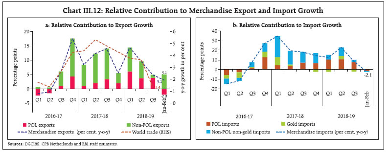
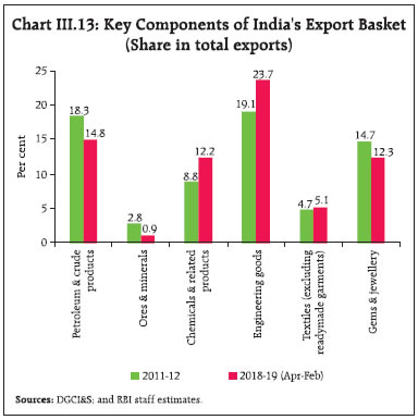 While the current account deficit (CAD) widened in H1:2018-19 to 2.6 per cent of GDP on the back of a higher trade deficit, softer international oil prices and robust earnings from services exports and remittances narrowed the CAD to 2.5 per cent of GDP in Q3. Under services, software exports rode on the upside of a significant improvement in export revenues of major IT companies in Q3. Optimistic forecasts of global IT spending in the next two years also portend well for the outlook of software exports. Lower outgo under income account also helped in containing CAD in Q3. 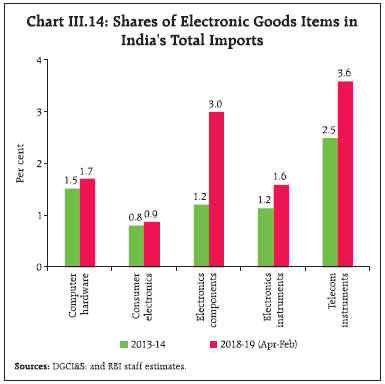 On the financing side, net foreign direct investment (FDI) flows at US$ 28.8 billion in 2018-19 (April-January) were higher than their level a year ago – flowing mainly into manufacturing, communication and financial services. Foreign portfolio investment – which made a flight to safety in 2018 due to concerns surrounding global growth, high oil prices and trade and geopolitical tensions – resumed in Q4, buoyed, inter alia, by dovish monetary policy stances in advanced economies. Flows under non-resident deposits and external commercial borrowings improved during the year. A new framework for external commercial borrowings was put in place in January 2019, which allowed a uniform borrowing limit of US$ 750 million a year across tenors and expanded the list of eligible borrowers. India’s net international investment position (NIIP) as a ratio to GDP deteriorated somewhat in December 2018 due to a rise in liabilities of domestic residents. India’s forex reserves at US$ 412.9 billion as on March 31, 2019 were at a comfortable level – equivalent to 9.5 months of imports and 182 per cent of short-term external debt (by residual maturity). III.2 Aggregate Supply The output growth, measured by gross value added (GVA) at basic prices, decelerated markedly to 6.3 per cent in H2:2018-19 from 7.3 per cent in H1 and 7.6 per cent a year ago (Table III.5). In contrast, its momentum measured in terms of q-o-q SAAR, accelerated to 6.7 per cent in H2 from 5.7 per cent in H1 (Chart III.15a). The slowdown in GVA growth (y-o-y) in H2:2018-19 was caused by a sharp deceleration in activity in agriculture and industry. Value added in agriculture decelerated to 1.4 per cent in H2, dropping to an eleven-quarter low in Q3 and further into contraction in Q4 (implied). Going by the second advance estimates of crop production, all major crops, except rice, sugarcane and oilseeds recorded lower production in 2018-19, than the record levels achieved in the preceding two years in succession. Keeping in view the pattern of revisions as national accounts move from advance estimates to revised estimates, some catch-up with the previous year’s level is likely. Industrial sector growth faced headwinds from subdued demand for manufacturing output and higher input costs due to an increase in oil prices in H1. Services sector activity, however, accelerated marginally, driven by resilience in construction activity and improvement in financial, real estate and professional services, and public administration, defence and other services (PADO), fuelled in part by a rise in government expenditure in H2:2018-19 (Chart III.15b). | Table III.5: Sector-wise Growth in GVA | | (y-o-y, per cent) | | Sector | 2017-18 (FRE) | 2018-19 (SAE) | Weighted Contribution 2018-19 | 2017-18 (FRE) | 2018-19 (SAE) | | Q1 | Q2 | Q3 | Q4 | Q1 | Q2 | Q3 | Q4# | | Agriculture, forestry and fishing | 5.0 | 2.7 | 0.4 | 4.2 | 4.5 | 4.6 | 6.5 | 5.1 | 4.2 | 2.7 | -0.1 | | Industry | 6.1 | 7.2 | 1.7 | -0.1 | 7.7 | 8.0 | 8.6 | 10.1 | 6.1 | 6.1 | 6.6 | | Mining and quarrying | 5.1 | 1.2 | 0.0 | 2.9 | 10.8 | 4.5 | 3.8 | 0.4 | -2.1 | 1.3 | 4.2 | | Manufacturing | 5.9 | 8.1 | 1.5 | -1.7 | 7.1 | 8.6 | 9.5 | 12.4 | 6.9 | 6.7 | 6.8 | | Electricity, gas, water supply and other utilities | 8.6 | 8.0 | 0.2 | 8.6 | 9.2 | 7.5 | 9.2 | 6.7 | 8.7 | 8.2 | 8.5 | | Services | 7.8 | 7.6 | 4.7 | 8.6 | 6.5 | 8.0 | 8.0 | 7.5 | 7.6 | 7.6 | 7.8 | | Construction | 5.6 | 8.9 | 0.7 | 3.3 | 4.8 | 8.0 | 6.4 | 9.6 | 8.5 | 9.6 | 8.1 | | Trade, hotels, transport, communication | 7.8 | 6.8 | 1.3 | 8.3 | 8.3 | 8.3 | 6.4 | 7.8 | 6.9 | 6.9 | 5.8 | | Financial, real estate and professional services | 6.2 | 7.3 | 1.6 | 7.8 | 4.8 | 6.8 | 5.5 | 6.6 | 7.2 | 7.3 | 8.2 | | Public administration, defence and other services | 11.9 | 8.5 | 1.1 | 14.8 | 8.8 | 9.2 | 15.2 | 7.6 | 8.7 | 7.6 | 10.0 | | GVA at basic prices | 6.9 | 6.8 | 6.8 | 5.9 | 6.6 | 7.3 | 7.9 | 7.8 | 6.8 | 6.3 | 6.3 | FRE: First Revised Estimates; SAE: Second Advance Estimates; #: Implicit growth.
Source: Central Statistics Office (CSO). |
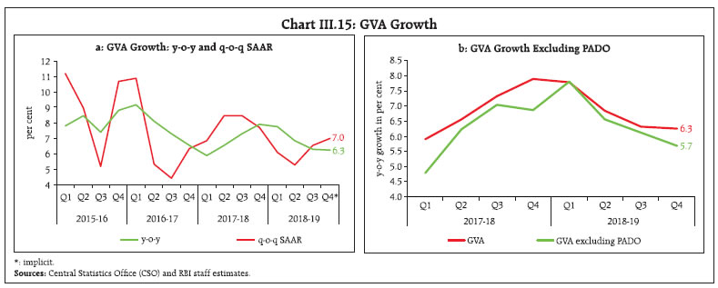 III.2.1 Agriculture GVA at basic prices in agriculture and allied activities decelerated in H2:2018-19 on account of a number of factors operating in conjunction, viz., the poor performance of the southwest and northeast monsoons, lower water reservoir levels in the eastern and western regions; unremunerative prices for farm produce depressed by the supply glut caused by two bumper harvests in succession and the lack of traction in food management policies to deal with large excess supplies, which led to heightened agrarian distress; and, unseasonal rains and hail storms. All these factors led to a shortfall of (-) 3.8 per cent in total rabi sowing from the previous year’s acreage. Consequent upon the release of the SAE of crop production for 2018-19, which indicated a minor upward revision in the production of kharif foodgrains but a lower-than-targeted rabi harvest, agricultural GVA growth for the year was revised downwards to 2.7 per cent from 3.8 per cent in the CSO’s first advance estimates (FAEs) (Table III.6). horticultural crop production was at a record level of 315 million tonnes during 2018-19, driven mainly by spices, aromatics and medicinal, flowers and vegetables. In the recent period, allied activities, which include livestock, forestry and fishing, have contributed around three-fourth of overall GVA growth of the sector (Chart III.16). As per the National Oceanic and Atmospheric Administration (NOAA) of the US, El Niño conditions strengthened during February 2019 as above-average sea surface temperatures increased across the equatorial Pacific Ocean. According to the latest report, there is a 80 per cent chance of El Niño prevailing in March-May, which will decrease to 60 per cent during the June-August period. Similarly, as per the Australian Bureau of Meteorology, the chance of El Niño developing in 2019 has increased to approximately 70 per cent. In case the monsoon turns out to be below normal, it may pose a downside risk to agricultural production, going forward. III.2.2 Industrial Sector In the industrial sector, gross value added at basic prices decelerated to 6.4 per cent in H2:2018-19 from 8.1 per cent in H1 and 8.3 per cent a year ago, pulled down by a fall in the growth of manufacturing activity as subdued demand was reflected in a moderation in sales growth (Chart III.17). | Table III.6: Agricultural Production in 2018-19 (Second Advance Estimates) | | (in Million Tonnes) | | Crop | 2017-18 | 2018-19 | 2018-19 Variation (Per cent) | | SAE | 4th AE | Target | SAE | Over SAE 2017-18 | Over 4th AE 2017-18 | Over Target | | Foodgrains | 277 | 285 | 290 | 281 | 1.4 | -1.2 | -3.1 | | Rice | 111 | 113 | 114 | 116 | 4.1 | 2.4 | 1.4 | | Wheat | 97 | 100 | 102 | 99 | 2.1 | -0.6 | -3.0 | | Pulses | 24 | 25 | 26 | 24 | 0.3 | -4.8 | -7.4 | | Oilseeds | 29.9 | 31.3 | 36.0 | 31.5 | 5.4 | 0.6 | -12.5 | | Sugarcane | 353.2 | 376.9 | 385.0 | 380.8 | 7.8 | 1.0 | -1.1 | | Cotton # | 33.9 | 34.9 | 35.5 | 30.1 | -11.3 | -13.8 | -15.2 | | Jute & Mesta ## | 10.5 | 10.1 | 11.2 | 10.1 | -4.1 | -0.6 | -10.1 | #: Million bales of 170 kgs. each.
##: Million bales of 180 kgs. each.
Source: Ministry of Agriculture and Farmers’ Welfare, Government of India. | IIP-based measures, viz., truncated index of industrial production (IIP), and IIP excluding digestive enzymes and antacids (DEA), also moderated during November-January 2018-19 (Chart III.18a). Manufacturing IIP decelerated in Q3:2018-19 due to a slowdown in production of motor vehicles, trailers and tractors, chemical and chemical products, rubber and plastics, coke and refinery products, textiles and beverages. Of the 23 industry groups constituting the IIP, ten contracted during Q3 as against four during Q2. In terms of the use-based classification, the production of infrastructure goods and consumer durables remained robust while consumer non-durables decelerated during Q3 (Chart III.18b). On the other hand, capital goods production contracted during Q3. The loss of speed in industrial output appears to have continued in Q4, with manufacturing growth slowing down to 1.3 per cent in January-February, 2019. In terms of use-based groups, construction/ infrastructure goods maintained pace in January, driven by strong growth of steel products. However, intermediate and capital goods production contracted, and consumer durables and consumer non-durables growth decelerated. 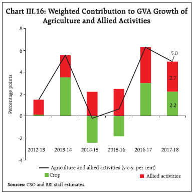
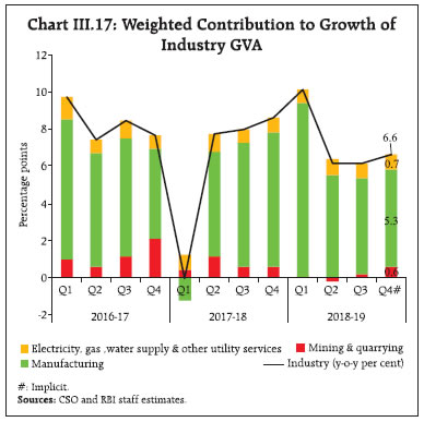
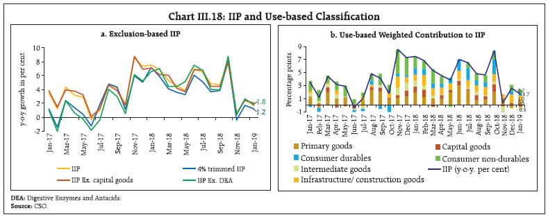 GVA in the electricity sector accelerated in H2 in comparison with H1. However, high frequency indicators suggest that electricity generation stagnated in January 2019 due to contraction in thermal power generation despite comfortable stocks of coal (Chart III.19). The slowdown in electricity generation was partly due to lean seasonal demand during January-February from the agriculture and household sectors on top of a slowdown in demand for electricity from industry during Q3. GVA growth in mining accelerated in H2 but was still lower than the growth in H2:2017-18. The Reserve Bank’s business assessment index of the industrial outlook survey (IOS) for Q3:2018-19 reflected a weakening of demand conditions in the manufacturing sector, although it points to an improvement in Q4. The manufacturing purchasing managers’ index (PMI) for March remained in expansion zone for the 20th month in succession on the back of increased output and new orders. III.2.3 Services Activity in the services sector picked up and became broad-based in H2:2018-19, boosted by resilience in construction activity and acceleration in financial, real estate and professional services and PADO (Chart III.20a). The strong performance of the construction sector was also reflected in its coincident indicators – steel consumption and cement production. Beginning December 2017, cement production registered double-digit growth in all months till January 2019, barring November 2018 (Chart III.20b). This was partly driven by the government’s focus on the road sector and affordable housing. 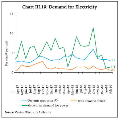
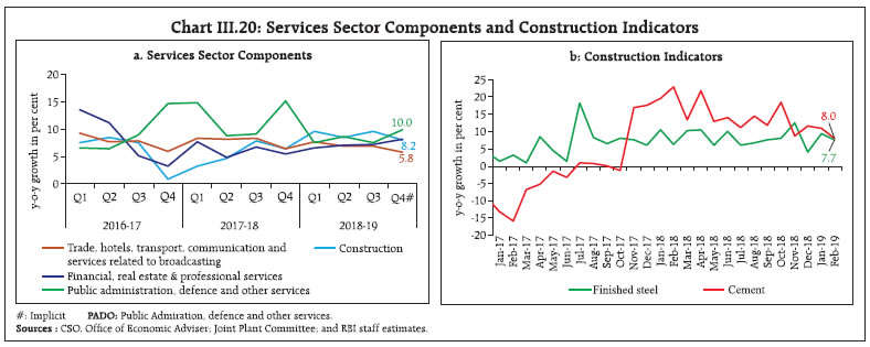 Growth in trade, hotels, transport, communication and services related to broadcasting was muted in H2:2018-19. Commercial vehicle sales – a lead indicator for road transport – plummeted due to rising fuel prices and relaxation of axle norms4. Other indicators for the transport sub-segment, viz., railway freight traffic and cargo handled at major ports, also decelerated in H2 (Chart III.21a). The growth of financial, real estate and professional services continued to accelerate with high frequency indicators of financial services extending their strong performance into Q4, supported by higher growth in personal loans and credit to the services sector as also the favourable base effect for aggregate deposits (Chart III.21b). 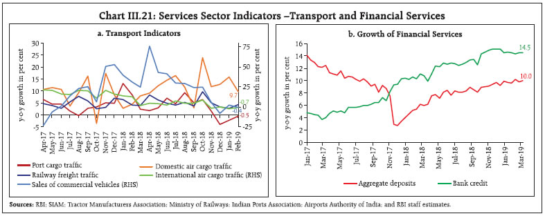 Among the other key constituents that provided support to services growth, PADO accelerated in H2:2018-19 due to higher value added by the states in the form of revenue expenditure (excluding interest payments). Real estate services continued to reel under deficient demand as reflected in stagnant sales and prices, decline in new launches across major cities, and still elevated, but reducing levels of unsold inventories (Chart III.22). Tax incentives for housing extended in the Union Budget 2019-20 are likely to improve demand, particularly in the affordable housing segment. III.3 Output Gap The output gap (i.e., deviation of actual output from its potential level expressed as a ratio of potential output) provides a summary measure of demand-supply conditions in the economy. As the output gap is an unobserved macroeconomic variable, considerable uncertainty exists about its true value, which poses a challenge for policy making. The uncertainty stems from large data revisions and the difficulty in distinguishing between cycle and trend in real time. Acknowledging these issues, a pragmatic approach is employed for assessing output gap estimates, combining eclectic methodologies, including different univariate filters – Hodrick- Prescott (HP); Baxter-King (BK); Christiano-Fitzgerald (CF); and multivariate Kalman filters (MVKF) taking into account inflation dynamics and financial factors, to derive a proximate view. This composite estimate suggests that a slight negative output gap opened in Q3 (Chart III.23a). This reflects deceleration in the pace of domestic demand, with real GDP growth decelerating from 8.1 per cent in Q4:2017-18 to 6.6 per cent in Q3:2018-19. However, the finance-neutral output gap (FNOG) – which factors in the behaviour of key financial variables such as bank credit, equity prices and policy repo rate – remained virtually closed in Q3:2018-19 (Chart III.23b). 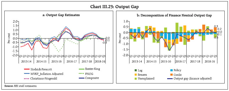 III.4 Conclusion The deceleration in economic activity which had set in during Q2, became entrenched in Q3. Going forward, several risks appear important. First, private consumption is expected to get a fillip from measures such as public spending in rural areas, and increase in disposable income of households due to income tax benefits. Second, resolution of stressed assets and plateauing of the level of non-performing advances (NPAs) on banking balance sheets are expected to improve credit flows, which augur well for improving economic activity. Third, improving capacity utilisation, tailwinds from lower oil prices and a policy rate cut in February are all likely to support economic activity. Nevertheless, several downside risks persist, both on the domestic and global fronts. The slowing down of the global economy may impact prospects of India’s exports. This risk may accentuate if trade tensions remain unresolved. Investment has been supported largely by government-led infrastructure spending. The key is to boost private investment across sectors, which will support demand in the short run, while boosting India’s growth potential over the medium-term.
IV. Financial Markets and Liquidity Conditions In the second half of 2018-19, financial market conditions were characterised by systemic liquidity needs being met through a mix of liquidity injection instruments with the weighted average call money rate (WACR) trading close to the policy rate in February-March; stock markets moving sideways though they rallied in March; bond yields tracking domestic developments and global spillovers; and the Indian Rupee appreciating due to easing of global crude prices and resumption of foreign portfolio inflows. Credit offtake continued to be buoyant with some moderation in interest rates on new loans since February 2019. Global financial market sentiment turned cautious during H2:2018-19 in the wake of rising trade tensions, concerns about a “no deal” Brexit and signs of slowing down of the global economy. Increased risk aversion and dovish monetary policy stances contributed to a decline in sovereign yields in the US, Germany and the UK. Credit spreads widened for corporate bonds in advanced economies (AEs) reflecting receding growth optimism, while equity valuations got trimmed as confidence diminished about earnings prospects. In the first quarter of 2019, equity markets in emerging market economies (EMEs) generally gained against the backdrop of waning trade tensions and country-specific factors. Despite the US Fed’s softer monetary policy stance from January 2019, the US$ retained an appreciating bias vis-à-vis other major AE currencies. IV.1 Domestic Financial Markets Divergent movements were observed in various segments of the domestic financial market as they reacted differently to the evolving global and local developments during H2:2018-19. In the overnight money market, interest rates remained close to the policy repo rate in February and March 2019 as the Reserve Bank injected liquidity through a mix of instruments. Yields on Treasury Bills (T-bills) moved in sync with longer tenor G-sec yields in response to global spillovers as well as domestic developments including (i) large infusion of liquidity through open market purchase operations; and (ii) large borrowing programme of the government announced in the Interim Budget 2019-20. Yields on corporate bonds broadly moved in line with those on government bonds. Equity markets moved sideways, but rallied sharply in March 2019. The exchange rate of the Indian Rupee (INR) traded with an appreciating bias as moderation in international crude oil prices, a dovish US Fed policy stance, waning trade tensions and the resumption of capital flows, buoyed appetite for emerging market assets. Credit flows from banks continued to improve and became increasingly broad-based. In response to a 25 bps reduction in the policy repo rate on February 7, 2019, some banks have reduced their lending rates under the marginal cost of funds-based lending rate (MCLR) system. IV.1.1 Money Market In the overnight money market, the weighted average call rate (WACR) generally remained below the policy repo rate during H2:2018-19, although it got increasingly aligned with the policy repo rate in February and March. The spread of the WACR over the policy rate moved in sync with the evolving liquidity conditions. As the liquidity conditions tightened, the spread narrowed in H2:2018-19 vis-a-vis H1 (see Section IV.3 for details). The volatility (standard deviation) of the WACR reduced to 0.1 per cent in H2:2018-19 from 0.2 per cent in H1. Other overnight money market rates moved in tandem with the WACR. The introduction of the triparty repo, which replaced the erstwhile Collateralised Borrowing and Lending Obligation (CBLO) from November 5, 2018, has ensured a level playing field in the money market as the triparty repo is exempted from maintenance of the cash reserve ratio (CRR), like the market repo, thereby obviating the sharp drops in CBLO rates on reporting Fridays. During H2:2018-19, the triparty repo and market repo rates remained below the WACR by 7 bps and 1 bps, respectively. During H2:2018-19, volumes have shifted somewhat from the market repo to call money and the triparty repo. The share of call and the triparty repo increased to 12.3 per cent and 65.7 per cent, respectively, in March 2019 from 8.2 per cent and 62.0 per cent, respectively, in October 2018 (before the introduction of the triparty repo). The share of the market repo declined from 29.8 per cent to 22.0 per cent during the same period (Chart IV.1). Interest rates on longer tenor money market instruments such as certificates of deposit (CDs), commercial papers (CPs) and 91-day Treasury Bills (T-bills) generally moved in sync during H2:2018-19 (Chart IV.2). After remaining elevated in September due to tight liquidity conditions, the 3-month T-bill rate softened in October mainly due to infusion of durable liquidity through OMOs. Rates on 3-month CPs and 3-month CDs eased in November, tracking T-bill rates. In Q3:2018-19, CP, CD and T-bill rates declined by 70 bps, 53 bps and 24 bps, respectively. These rates softened by 15 bps, 21 bps and 21 bps, respectively, on February 8, 2019 consequent to the policy repo rate reduction. Though T-bill rates continued to decline in Q4, 3-month CD and 3-month CP rates hardened by 31 bps and 23 bps, respectively, in anticipation of tightening of liquidity conditions in March 2019 due to the usual financial year-end effects. Fresh issuances of CDs increased to ₹3,030 billion during H2:2018-19 (up to March 15, 2019) as compared with ₹2,482 billion during the corresponding period of 2017-18. 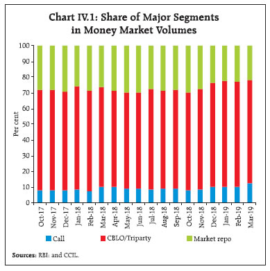 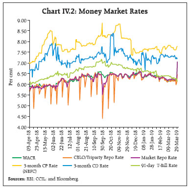 Issuances of CPs declined marginally to ₹12,383 billion in H2:2018-19 from ₹12,447 billion in H2:2017-18 mainly due to heightened risk aversion post the Infrastructure Leasing & Financial Services Limited (IL&FS) debt event. Primary issuances of CPs, which declined from September 2018 consequent to a series of rating downgrades of IL&FS and its associated companies, started recovering from November (Chart IV.3a) led by non-bank financial companies (NBFCs) and non-bank private corporates (Chart IV.3b). Interest rates in the primary CP market, which hardened from August until mid-November, softened thereafter by about 35 bps by the end of March 2019. IV.1.2 Government Securities (G-sec) Market At the beginning of H2:2018-19, benchmark yields increased by 12 bps due to concerns about exchange market pressures. Yields softened by 13 bps in early October as the RBI maintained status quo on the policy rate, which surprised the market, and this downward movement was reinforced by the decline in international crude prices. Yields shed this softness, however, and spiked by 10 bps on October 9, 2018 as the INR depreciation sparked fears of a large sell-off by foreign portfolio investors (FPIs). These concerns abated as the rupee recovered after India’s trade deficit for September fell to its lowest level in five months, followed by an announcement of open market purchases by the RBI. Lower inflation prints accompanied by a sharp decline in crude oil prices resulted in a decline in yields by 10 bps during the first half of November. On November 16, yields rebounded by 6 bps on the back of a sharp rise in oil prices. On November 22 and November 28, yields fell by 8 bps and 9 bps, respectively, due to (i) a continuing fall in crude oil prices; and (ii) buoyed sentiments after the announcement of multiple open market purchases by the RBI till end-December. During December 2018, yields on the benchmark paper fell by 24 bps to 7.37 per cent, notwithstanding intermittent hardening because of fears about fiscal slippages on account of the farm relief package and an expected rise in market borrowing during 2019-20. Overall, the benchmark yield fell by 65 bps during Q3:2018-19. The benchmark yield rose by 11 bps during January 2019 amidst deteriorating market sentiments sparked by (i) concerns about the fiscal position of the central government; and (ii) a rise in crude oil prices due to the crude oil production cuts by Organisation of the Petroleum Exporting Countries (OPEC) and others. It moderated by end-January 2019 due to absence of details on widely expected farm relief package from the centre. The announcement of additional borrowing of ₹1,390 billion for 2019-20 over and above the revised estimate of 2018-19 in the Interim Budget 2019-20 led to a firming up of the yield on the new benchmark paper (7.26% GS 2029) by 9 bps to 7.38 per cent and the old benchmark paper (7.17% GS 2028) by 13 bps to 7.61 per cent. Nevertheless, the reduction in the repo rate by the Reserve Bank, which was unanticipated by the market, and the downward revision of the projected inflation trajectory for April to September 2019 resulted in a decline in the new benchmark by 4 bps to 7.32 per cent and the old benchmark by 7 bps to 7.50 per cent. Furthermore, expectations of another rate cut in April, triggered by the CPI falling to its nineteenth month low of 2.1 per cent (provisional) in January 2019, led to a decline in the benchmark yield1. New and old benchmark yields, however, hardened by 12 bps and 13 bps, respectively, in the third week of February due to concerns of a sharp increase in supply of goverment-securities (Chart IV.4). Yields during March was steady with a softening bias on expectations of monetary policy easing, improvement in liquidity conditions, announcement of Voluntary Retention Route (VRR) for FPIs, benign inflation data and infusion of liquidity through USD/INR buy/sell swap auction. The yield curve underwent a level shift in H2:2018-19 in response to both global spillovers and domestic factors such as lower crude oil prices, moderation in the domestic inflation outlook, monetary policy measures and shift in the stance (Chart IV.5). The reduction in the repo rate in February resulted in a perceptible downward shift of the yield curve, both at the short and medium tenor segments (up to 7 years) and at the longer end (beyond 20 years). In October 2018 and January 2019, FPIs remained net sellers in the G-sec market, but they turned net buyers during November-December with the easing of crude oil prices and the return of risk-on sentiment. From October 2018 till March 2019, FPIs made net purchases of ₹50.5 billion in the debt segment, of which state development loans (SDLs) constituted ₹0.2 billion. During March, FPIs made net purchases amounting to ₹339.8 billion in the equity segment and ₹120.0 billion in the debt segment (Chart IV.6). At the shorter end of the primary market segment, yields on T-Bills tracked the benchmark yield and hardened at the beginning of H2:2018-19 but they regained a softening bias in February on declining crude oil prices and the reduction in the policy repo rate (Chart IV.7). During March, yields on T-Bills softened on expectations of further rate cut, improvment in liquidity conditions due to open market operations and USD/INR buy/sell swap auction. At the longer end, the issuance of SDLs increased during H2:2018-19. The weighted average spread of SDLs’ cut-off rate over G-sec yield increased to 65 bps in H2:2018-19 from 54 bps in H1:2018-19 (Chart IV.8). The average inter-state spread on securities of 10-year tenor was higher at 7.5 bps during H2:2018-19 as against 4 bps in H1:2018-19. IV.1.3 Corporate Bond Market Corporate bond yields largely tracked G-sec yields during H2:2018-19. The AAA 5-year corporate bond yields softened by 76 bps from 8.86 per cent at end-September 2018 to 8.10 per cent at end-March 2019 (Chart IV.9a). Despite the softening, however, the spread of 5-year AAA corporate bond yield over 5-year G-sec yield increased by 58 bps during the period, reflecting increased credit risk premia in the aftermath of the IL&FS episode and liquidity squeeze faced by some non-banking financial companies (NBFCs). Consequent to the Reserve Bank’s announcement to inject rupee liquidity through long-term foreign exchange buy/sell swap auction, however, both the yield and the spread declined sharply. Credit default swap (CDS) spreads on State Bank of India and ICICI Bank papers declined during the period. 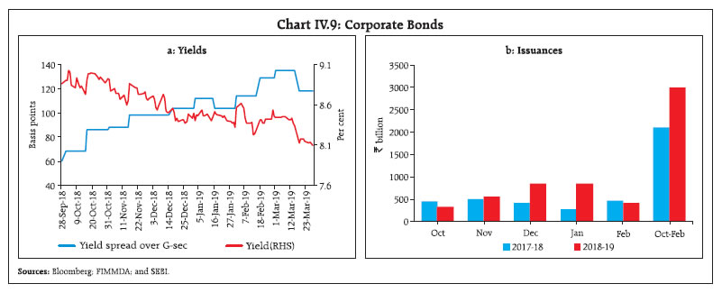 The average daily turnover in the corporate bond market increased to ₹80 billion during H2:2018-19 from ₹76 billion a year ago. The softening of corporate bond yields encouraged corporates to resort to increased bond issuance in December 2018 and January 2019, although it moderated in February 2019. Overall, resource mobilisation through issuances of corporate bonds in the primary market increased by 42.0 per cent to ₹2.99 trillion during October 2018 - February 2019 from ₹2.11 trillion a year ago (Chart IV.9b). Almost the entire resource mobilisation of the corporate bond market (98.6 per cent) continued to be through the private placement route. Investments by FPIs in corporate bonds increased to ₹2.2 trillion at end-March 2019 from ₹2.0 trillion at end-September 2018, with sizeable investments in the month of March 2019. Consequently, FPIs’ utilisation of the approved limit for investment in corporate bonds increased to 75.9 per cent at end-March 2019 from 75.5 per cent at end-September 2018. IV.1.4 Equity Market The Indian equity market, which was buoyant till August 2018, fell sharply during September, triggered by the unfolding of the IL&FS episode. The downturn got exacerbated in October as market sentiment was dented by the liquidity tightness in the NBFC sector, coupled with global trade tensions. The market staged a short-lived turnaround in November 2018 mainly due to easing of liquidity concerns in the NBFC sector. Since then, markets have exhibited two-way movements (Chart IV.10.a), but rallied sharply in the month of March 2019 leading to India outperforming most of its peers among major EMEs and some AEs (Chart IV.10b). Overall, the BSE Sensex increased by 6.8 per cent in rupee terms and 11.7 per cent in dollar terms during H2:2018-19. A combination of both domestic and global factors, concerns relating to trade tensions between the US and China, a sharp depreciation of the INR vis-à-vis the US$ against the backdrop of higher oil prices and widening of India’s current account deficit for Q1:2018-19, kept the equity market under pressure in October 2018 (Chart IV.11a). A turnaround occurred during November 2018 on easing of concerns over liquidity tightness, waning inflation pressures, expectations of a breakthrough in the US-China trade relations at the G-20 summit, dovish statement by the US Fed, improvement in India’s ranking in the World Bank’s ease of doing business index and a sharp appreciation of the rupee against the US dollar. 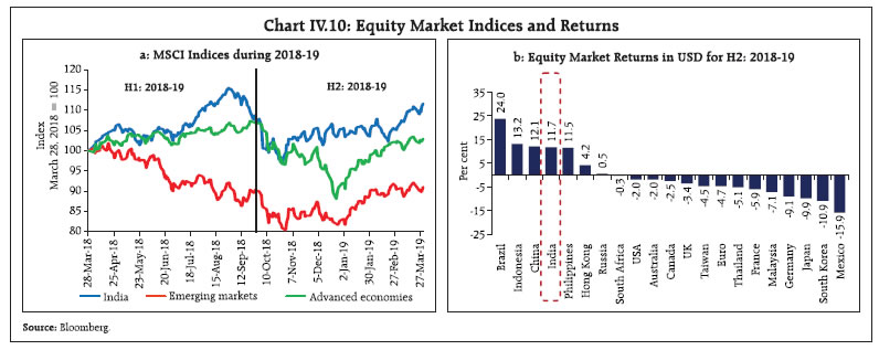 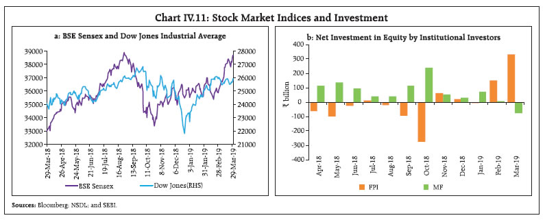 Amidst heightened volatility, the equity market declined moderately in December 2018 due to a combination of factors, including weaker than expected Q2:2018-19 GDP growth, uncertainty regarding the outcome of state assembly elections and the fourth interest rate hike in a year by the US Fed. After declining for the most part of January 2019 on negative global cues emanating from slowing Chinese growth and a weaker global growth outlook, the BSE Sensex increased by 1.9 per cent on January 31, 2019 mainly because of the US Fed’s decision to hold rates along with the indication that it would adopt a patient approach to further rate hikes. Positive expectations from the Interim Budget, 2019-20 and domestic monetary policy contributed to the rally. Market sentiment, however, reversed during February 2019 due to partial US government shutdown, concerns over the US-China trade talks and India-Pakistan tensions. The market rebounded sharply in the month of March 2019 as it increased by 7.8 per cent on the back of positive global cues, easing of cross-border tensions, increasing optimism about general election outcome and large investments by FPIs. Both domestic institutional investors, particularly mutual funds (MFs), and FPIs were the net buyers in the equity market. Net purchases by MFs and FPIs in equities amounted to ₹326 billion and ₹288 billion, respectively, during H2:2018-19 (Chart IV.11b). In the primary segment of the equity market, resource mobilisation through public issues of equity (initial public offers and right issues) declined by 93 per cent to ₹58.5 billion during September 2018-February 2019 as compared with ₹781.5 billion in the corresponding period of the previous year. IV.1.5 Foreign Exchange Market Since October 2018, the INR has traded with an appreciation bias, recovering from a historical low of ₹74.4 per US$ (reference rate) on October 11, 2018 to ₹69.2 per US$ on March 29, 2019 (Table IV.1). Moderation in international crude oil prices, the dovish policy stance of the US Fed and waning of trade concerns helped many EMEs currencies appreciate against the US dollar in H2:2018-19. | Table IV.1: Nominal and Real Effective Exchange Rates: Trade-based (Base: 2004-05 = 100) | | Item | Index: end-Mar 2019 (P) | Appreciation (+) / Depreciation (-) (Per cent) | | end-Mar 2019 over end-Sep 2018 | | 36-currency REER | 116.6 | 5.3 | | 36-currency NEER | 74.1 | 4.9 | | 6-currency REER | 123.5 | 4.3 | | 6-currency NEER | 64.3 | 5.0 | | ₹/ US$ (As on March 29, 2019) | 69.2 | 4.9 | P: Provisional.
Note: REER figures are based on the Consumer Price Index (Combined).
Source: RBI. | The narrowing of the trade deficit, benign inflation outlook and recovery in FPI investment flows helped attenuate pressure on the domestic foreign exchange market. Turkish Lira witnessed the highest appreciation followed by the INR and the Indonesian Rupiah in H2:2018-19 over H1:2018-19 (Chart IV.12a). The volatility in INR, as measured by the coefficient of variation, was lower at 2.0 in H2:2018-19 as compared with 3.0 in H1:2018-19. While the INR has appreciated by 4.9 per cent against the US dollar since end-September 2018, it has appreciated by 8.7 per cent against the euro and 4.9 per cent against the pound sterling. In terms of both the nominal effective exchange rate (NEER) and the real effective exchange rate (REER), the INR has appreciated by 4.9 per cent and 5.3 per cent, respectively, since end-September 2018 (Chart IV.12b). IV.1.6 Credit Market In the credit market, non-food credit growth (y-o-y) accelerated to 15.2 per cent in November 2018, its highest level in the last five years (Chart IV.13a). Although quarterly growth in non-food credit moderated in Q3:2018-19 vis-a-vis Q2:2018-19, it recovered in Q4 with the year-on-year (y-o-y) growth being higher at 14.4 per cent (up to March 15, 2019) than 11.0 per cent a year ago (Chart IV.13b). Credit extended by public sector and foreign banks recovered gradually during H2:2018-19 (Chart IV.14). Of the incremental credit extended by scheduled commercial banks as on March 15, 2019, 47.4 per cent was provided by public sector banks, 48.9 per cent by private sector banks and 3.7 per cent by foreign banks. Incremental credit flows are also getting increasingly broad-based, with services accounting for the highest share (in February 2019) as against personal loans a year ago (Chart IV.15). Credit growth to industry, which turned positive in November 2017 after more than a year-long contraction, improved, particularly in respect of infrastructure, chemical and chemical products, engineering and petroleum, coal products and nuclear fuels. The share of credit to agriculture, however, moderated. While the overall non-performing assets (NPA) ratio of SCBs moderated in December in comparison with the position at end-March 2018, it deteriorated in the case of personal loans and agriculture, the sectors that received large credit flows in recent years (Chart IV.16a). In contrast, the NPA ratio dipped in December in the case of industry and services as compared with March 2018 (Chart IV.16b). Banks’ investments in CPs, bonds, debentures and shares of public and private corporates, which are reflected in non-SLR investments, were higher during H2:2018-19 (up to March 15) than a year ago mainly due to higher investments in bonds/ shares and debentures (Chart IV.17a). As a result, adjusted non-food credit2 growth was higher in Q4 vis-à-vis Q3:2018-19 (Chart IV.17b). With increased flow of credit and an increase in non-SLR investments, excess SLR maintained by banks in H2:2018-19 moderated vis-à-vis H1 levels (Chart IV.18). Apart from increased credit offtake from banks, financial flows to the commercial sector from other sources also increased, contributed mainly by external commercial borrowings, foreign direct investment and an almost four-fold increase in issuances of CPs (Table IV.2). The total flow of financial resources to the commercial sector in 2018-19 (up to March 15, 2019) from bank and non-bank sources increased significantly as compared with the corresponding period a year ago (Chart IV.19). IV.2 Monetary Policy Transmission Monetary transmission to the deposit and lending rates of commercial banks was partial and delayed. In response to the increase in the policy repo rate by 50 bps (25 bps each in June and August 2018), the weighted average lending rate (WALR) on fresh rupee loans increased by 53 bps (since June 2018), but the extent of rise in lending rates on outstanding rupee loans was muted (13 bps), attributable to the lending behavior of public sector banks. Following the reduction in the policy repo rate by 25 bps on February 7, 2019, the WALR on fresh rupee loans declined by 12 bps during February 2019 notwithstanding a muted response to deposit rates and the 1-year median MCLR of commercial banks (Table IV.3). 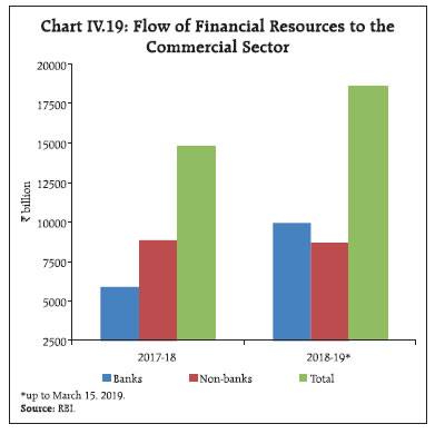
| Table IV.2: Funding from Non-Bank Sources to the Commercial Sector | | (₹ billion) | | Items | April to March # | | 2017-18 | 2018-19 | | Amount | Per cent to Total | Amount | Per cent to Total | | A. Flow from Non-banks (A1+A2) | 8,869 | 100.0 | 8,683 | 100.0 | | A1. Domestic Sources | 6,515 | 73.5 | 5,532 | 63.7 | | 1. Public issues by non-financial entities | 360 | 4.1 | 102 | 1.2 | | 2. Gross private placement by non-financial entities $ | 1,305 | 14.7 | 1,209 | 13.9 | | 3. Net issuance of CPs subscribed by non-banks | 453 | 5.1 | 1,767 | 20.3 | | 4. Net credit by housing finance companies | 1,452 | 16.4 | 1,186 | 13.7 | | 5. Total accommodation by 4 RBI regulated AIFIs $ | 706 | 8.0 | 960 | 11.1 | | 6. NBFCs-ND-SI (net of bank credit) | 1,959 | 22.1 | 128 | 1.5 | | 7. LIC's net investment in corporate debt, infrastructure and social sector $ | 280 | 3.2 | 181 | 2.1 | | A2. Foreign Sources | 2,353 | 26.5 | 3,151 | 36.3 | | 1. External Commercial Borrowings / FCCB * | -72 | -0.8 | 418 | 4.8 | | 2. Short-term credit from abroad^ | 294 | 3.3 | 102 | 1.2 | | 3. Foreign Direct Investment to India * | 2,131 | 24.0 | 2,631 | 30.3 | *: Up to January 2019 $: Up to February 2019; ^: Up to September 2018; #: Up to March 15, 2019.
Sources: RBI; SEBI; BSE; NSE; NHB; LIC and merchant banks. |
| Table IV.3: Transmission to Deposit and Lending Rates | | (Basis points) | | Period | Repo Rate | Term Deposit Rates | Lending Rates | | Median Term Deposit Rate | WADTDR | 1 - year Median MCLR | WALR - Outstanding Rupee Loans | WALR - Fresh Rupee Loans | | January 2018 to January 2019 | 50 | 29 | 38 | 50 | 2 | 52 | | Tightening Cycle: | | | | | | | | June 2018 to January 2019 | 50 | 18 | 20 | 32 | 13 | 53 | | Easing Cycle: | | | | | | | | February – March 2019 | -25 | -3 | -1 | -5 | -2 | -12 | WADTDR: Weighted Average Domestic Term Deposit Rate. WALR: Weighted Average Lending Rate.
MCLR: Marginal Cost of Funds based Lending Rate. Latest data for WADTDR and WALR pertain to February 2019.
Source: RBI. | Public sector banks reduced the WALR on outstanding rupee loans during the tightening phase of monetary policy (June 2018 - January 2019) due to their inability to pass on the increase in the cost of funds to lending rates, possibly due to mis-pricing of credit risk in their loan portfolio (Chart IV.20a). Consequently, the spread between the WALR and the weighted average domestic term deposit rates (WADTDR) of public sector banks declined (Chart IV.20b). In contrast, private sector banks were able to maintain a higher spread (WALR over WATDR) vis-à-vis public sector banks, reflective of their better pricing power even though the rise in term deposit interest rates offered by private sector banks was higher than that of public sector banks. The spreads (WALR over 1-year median MCLR) charged by private sector banks were much higher than those charged by public sector banks in February 2019; however, credit extended by private sector banks continued to expand at a faster pace than that by public sector banks (Chart IV.14 and IV.21a & b). In keeping with the usual pattern of pricing of credit, the spread charged was lowest for loans to the housing sector which involve relatively low default risk. On the other hand, the spread was highest for personal loans (other than housing, vehicle and education), which carry high risk (Chart IV.22). In the housing sector, banks face stiff competition from housing finance companies (HFCs) (Chart IV.23). As such, banks charge a lower spread on such loans. The spread between WALR on fresh rupee loans/ outstanding rupee loans and bond yields has risen since September 2018, reflecting an increase in pricing power due to strengthening of credit demand (Chart IV.24). Following the reduction in the policy rate by 25 bps in February 2019, 38 banks have reduced their 1-year MCLR so far (till end-March 2019) in the range of 1-106 bps. However, 24 banks, mostly foreign banks, increased their MCLR in the range of 5-113 bps during the same period. While the median term deposit rate (all maturities) of banks declined by 3 basis points, the 1-year median MCLR declined by 5 bps during the easing phase so far. IV.3 Liquidity Conditions and the Operating Procedure of Monetary Policy The RBI Act, 1934 amended in 2016 requires the RBI to place the operating procedure relating to the implementation of monetary policy and changes thereto from time to time, if any, in the public domain. During 2018-19, liquidity management operations by the RBI were aligned with the broad framework discussed in the Monetary Policy Reports of April 2018 and October 2018. During H2:2018-19, the RBI continued to fine-tune liquidity through variable rate auctions of both repos and reverse repos, in addition to the regular operations. While liquidity amounting to ₹4,103 billion was injected through variable rate repos of maturities ranging from overnight to 56-day in addition to the regular 14-day repos, liquidity amounting to ₹27,376 billion was absorbed through reverse repos of overnight to 7-day maturity. In view of the need to inject durable liquidity warranted by large leakage through currency expansion and forex operations, the RBI conducted twenty-two open market operation (OMO) purchase auctions aggregating ₹2,485 billion during H2:2018-19, taking the total infusion of liquidity through OMOs to ₹2,985 billion during 2018-19. Based on an assessment of financial market conditions, the RBI increased the Facility to Avail Liquidity for Liquidity Coverage Ratio (FALLCR) effective October 1, 2018, which supplemented the ability of individual banks to avail liquidity from the repo market against high-quality collateral. Furthermore, it was decided to reduce the statutory liquidity ratio (SLR) by 25 bps every calendar quarter until it reaches 18 per cent of NDTL to align the SLR with the liquidity coverage ratio (LCR) requirement. The first round of reduction of 25 bps became effective from the quarter commencing January 2019, lowering the SLR to 19.25 per cent of NDTL. Drivers and Management of Liquidity Leakage of liquidity from the banking system by way of increase in Currency in Circulation (CiC) was the main driver of liquidity in H2:2018-19. This was in contrast to H1 when the main driver of liquidity was RBI’s forex operations, necessitated by capital outflows (Chart IV.25). On a year-on-year basis, average CiC growth of 20.4 per cent during Q3:2018-19 was significantly higher than the nominal GDP growth of 11.0 per cent for the third quarter. Weekly expansion in CiC of ₹494 billion around Diwali (November 7, 2018) was unprecedented (Chart IV.26). During Q4, CiC expanded by ₹1,147 billion, taking the total expansion in CiC to ₹2,144 billion in H2. Expansion in CiC is driven largely by macroeconomic factors such as nominal GDP growth and interest rates over the medium term. In the short term, however, it is also influenced by seasonal factors such as festivals and idiosyncratic factors like demonetisation and elections (Box IV.1). In the second week of October, a large increase in currency demand and RBI’s forex sales resulted in a systemic liquidity deficit, which continued for the rest of the month. With the Government resorting to ways and means advances (WMA) to finance higher spending, the deficit moderated at the beginning of November but increased subsequently because of higher currency expansion during the festival season. The liquidity deficit increased in the second half of December mainly due to advance tax outflows. To meet liquidity needs, the RBI conducted variable rate repo auctions of longer tenors (28-56-day) in addition to the regular 14-day repos. Additionally, durable liquidity of ₹360 billion was injected through OMOs in October 2018, which was subsequently scaled up to ₹500 billion each in November and December, taking the total durable liquidity injection to ₹1,360 billion (through twelve auctions) during the quarter (Chart IV.27). 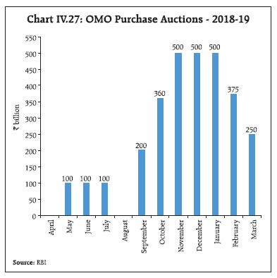 Deficit liquidity conditions persisted in Q4:2018-19 in the wake of sustained currency expansion and the build-up of government cash balances, barring a few days at the beginning of both January and February when liquidity conditions were in surplus as the government resorted to overdraft (OD)/ways and means advances (WMA). To meet durable liquidity needs, the RBI conducted OMO purchases of ₹500 billion in January, ₹375 billion in February and ₹250 billion in March. Simultaneously, transient liquidity needs were met through variable rate repos of various tenors in addition to the regular 14-day term repos. Sporadic instances of excess liquidity were managed through variable rate reverse repos of different tenors (Chart IV.28). Box IV.1: Modelling Currency Demand Globally, central banks estimate and forecast currency movements for liquidity management operations (Khatat, 2018). The demand for currency at the aggregate level is estimated at both the quarterly and monthly frequency to distinguish between the long-term and short-term determinants3. In the long run, the demand for currency depends upon key macroeconomic variables (e.g., nominal GDP, interest rates, etc.) which enables identification of shifts in currency demand over time. In the short-run, the demand for currency is mainly driven by seasonal factors (including festival demand) and some idiosyncratic factors (for instance, elections), the patterns of which could be identified from historical data (Nachane et al., 2013; Bhattacharya and Singh, 2018). To understand the long-run relationship between the demand for currency in circulation and its major macroeconomic determinants such as output and the interest rate, empirical analysis is undertaken using quarterly data spanning Q2:1998 to Q3:2018. Both currency and gross domestic product are converted into logarithmic form. Dummies are used to capture the impact of festivals and demonetisation. The autoregressive distributed lag (ARDL) model was used, keeping in view the different orders of integration of the data series (Pesaran et al., 2001), with the following specification (Raj et al., 2019):  The long-run relationship between the demand for currency and its determinants indicates that the income elasticity of currency demand is marginally above unity during the period under consideration (Table IV.1.1). As expected, currency demand is negatively related to ADR, although the effect is muted (though statistically significant). Apart from these fundamental variables, currency demand is influenced by several frictional factors such as festivals, elections and one-off events such as demonetisation. Finally, the short-run dynamics captured by the error correction term indicate that the speed of adjustment to any shock is significant, i.e., around 28 per cent of the deviation gets adjusted in the following quarter. To check the empirical regularity of this phenomenon at a higher frequency, a model using monthly data for the period April 2004 to December 2018 was estimated through an autoregressive process to control for persistence in currency demand. Dummies representing festivals/elections and demonetisation were also used in the following specification:  where the growth in Log of CiC (m-o-m, per cent) represent the dependent variable, Ei represent a dummy variable for the ith month before general elections, E0 is the dummy for the month in which general elections were held and Ej represents a dummy in the jth month after the general elections. The growth in currency demand is found to exhibit some persistence (Table IV.1.2). Regression coefficients for the monthly dummies before the general elections were positive (but statistically insignificant), while they were found to be positive and statistically significant during election months, suggesting an increase in currency demand during those months. Post-election month dummies, however, turned out to be to be negative (and statistically significant) indicating the return of CiC to the banking system. Dk representing dummies to capture the impact of demonetisation for the kth period were found to be significant, i.e., while money returned to the system in the first two months of demonetisation, re-monetisation started from the third and lasted till the fifth month. As expected, CiC picks up during the festival months of October/ November (Dussehra and Diwali). | Table IV.1.1: Long-run Determinants | | Long-run Equation Dependent Variable (CiC) | ARDL (4, 4, 4) | | LNGDP | 1.04 (0.00) | | ADR | - 0.03 (0.03) | | D_DEMO | - 0.17 (0.00) | | D_FEST | 0.14 (0.04) | | Memo items: | | | Diagnostics | | | Error correction (-1) | - 0.28 (0.00) | | Adjusted R-squared | 0.98 | | F-Statistics | 6.26 | | Lower and upper bound critical value | 1% [4.13 5.00] | | Q-statistic | 1.77 (0.18) | Note: Figures in parentheses indicate p-value. Lag length is selected using Akaike Information Criteria (AIC).
Source: RBI Staff estimates. |
| Table IV.1.2: Short-term Determinants | | Dependent Variable: ΔLCiC | | Variables | Coefficient | t-Statistic | Probability | | ΔLCiC(-1) | 0.31 | 5.64 | 0.00 | | DEMO_D1 | -0.42 | -32.36 | 0.00 | | DEMO_ D2 | -0.12 | -4.61 | 0.00 | | DEMO_ D3 | 0.15 | 7.80 | 0.00 | | DEMO_ D4 | 0.10 | 7.76 | 0.00 | | DEMO_ D5 | 0.09 | 6.10 | 0.00 | | D_FEST | 0.02 | 4.99 | 0.00 | | D_GEL-E1 | 0.09 | 1.03 | 0.31 | | D_GEL-E2 | 0.33 | 0.44 | 0.66 | | D_GEL | 0.02 | 3.16 | 0.00 | | D_GEL+ E1 | -0.02 | -2.08 | 0.04 | | D_GEL+ E2 | -0.02 | -2.66 | 0.01 | | C | 0.01 | 5.38 | 0.00 | | R-squared | 0.94 | Adjusted R-squared | 0.90 | | F-Statistics | 142.82 | Durbin-Watson stat | 2.06 |
The robustness of both the models is evident from the plot of the actual and the estimated values derived from both quarterly and monthly models (Chart IV.1.1). References: Bhattacharya, K., and S. K. Singh (2018), “The Story of Currency in Circulation: Are We Back to Square One after Demonetisation?”, Economic & Political Weekly Vol. LIII No. 13, March. Khatat, M. E. H. (2018), “Monetary Policy and Models of Currency Demand”, IMF Working Paper 18/28, February. Nachane, D. M., A. B. Chakraborty, A. K. Mitra and S. Bordoloi (2013), “Modelling Currency Demand in India: An Empirical Study”, RBI DRG Study No. 39, February. Pesaran, M., Shin, Y., and Smith, R. (2001), “Bounds testing approaches to the analysis of level Relationships”, Journal of Applied Econometrics, 16, 289–326. Raj, J., I. Bhattacharyya, S. R. Behera and B. A. Talwar (2019), “Modelling Currency Demand in India”, RBI Mimeo. |
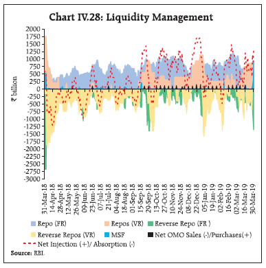 To sum up, the RBI’s forex operations and currency expansion were the prime drivers of durable liquidity in the banking system in 2018-19, while government spending was the key driver of frictional liquidity movements. Since the Reserve Bank regularly injected durable liquidity through OMOs, net LAF positions mirrored largely movements in government cash balances (Chart IV.29). | Table IV.4: Key Liquidity Indicators during 2018-19 | | (Number of days*) | | Month | Net LAF | GoI Cash Balances | Deficit
(repo) | Surplus
(reverse repo) | Build-up | Drawdown | | April | 1 | 18 | 19 | 0 | | May | 5 | 17 | 18 | 4 | | June | 10 | 11 | 4 | 17 | | July | 16 | 6 | 6 | 16 | | August | 10 | 10 | 6 | 14 | | September | 12 | 6 | 9 | 9 | | October | 17 | 4 | 9 | 12 | | November | 18 | 0 | 4 | 14 | | December | 19 | 1 | 13 | 7 | | January | 20 | 3 | 6 | 17 | | February | 15 | 4 | 15 | 4 | | March | 19 | 0 | 12 | 7 | *: Working days excluding Saturdays.
Source: RBI. |
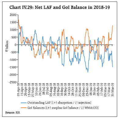 Movements in government cash balances are directly reflected in LAF positions on most occasions. While drawdown of cash balances by the government resulted in surplus liquidity, which was absorbed through reverse repo under the LAF window, the build-up of government cash balances resulted in deficit, which was managed through repo operations (Table IV.4). The temporary mismatches between receipts and payments of the government during H2:2018-19 were met through its recourse to cash management bills (CMBs) on four occasions of maturity ranging 12-59 days aggregating ₹1,050 billion. Fine-tuning operations through variable rate auctions was another defining feature of liquidity management during H2:2018-19. Large liquidity injections were made through repo auctions of maturities ranging from overnight to 56 days, while reverse repos of maturities ranging from overnight to 7 days were frequently used for absorbing liquidity (Table IV.5). The evolution of liquidity conditions and their management by the RBI gets encapsulated in the movement of bank reserves, which evolve largely through the dynamic interaction between the central bank and depository institutions. If liquidity pressures from autonomous drivers of liquidity are not fully (more than) offset by liquidity management measures, they are reflected in drawdown (accumulation) of bank reserves. An analytical scrutiny of the liquidity drivers and their management during 2018-19 provides some interesting insights. During H2:2018-19, liquidity withdrawal through autonomous drivers was more than offset through liquidity management operations. Consequently, there was an increase in bank reserves unlike H1 (Table IV.6). Thus, an aggregate picture of bank reserves for the full year may not be reflective of intra-year liquidity dynamics. | Table IV.5: Fine-tuning operations through variable rate auctions in H2:2018-19 | | | Repo (maturity in days) | Reverse Repo (maturity in days) | | 1-3 | 7 | 14 | 21 | 28 | 55-56 | 1 | 2 | 3 | 4 | 7 | | Frequency (number of days) | 4 | 4 | 2 | 2 | 2 | 4 | 41 | 5 | 13 | 2 | 31 | | Average volume (₹ billion) | 215.1 | 234.6 | 126.9 | 325.0 | 225.0 | 237.5 | 392.1 | 403.4 | 405.3 | 246.3 | 113.6 | Operating Target and Policy Rate The objective of liquidity management is to align the WACR – the operating target – with the policy repo rate. In H2:2018-19, the WACR generally traded below the policy repo rate during October-January but hardended intermittenly thereafter and spiked at the year-end (Chart IV.30). During H2:2018-19, the negative spread of the WACR over the repo rate increased from 5 bps in October to 12 bps in January (Chart IV.31). Post announcement of reduction in the repo rate by 25 bps on February 7, 2019, however, the WACR aligned closer to the repo rate in February and March. Overall, the WACR, on average, remained 6 bps below the policy repo rate in H2 as against 10 bps in H1:2018-19. The WACR traded below the repo rate even after systemic liquidity turned tight beginning Q2:2018-19 warranting net injection through repos (Table IV.7). This anomalous behaviour can be attributed to three factors. First, most of the co-operative banks are not participants in the NDS-Call trading platform. Non-scheduled co-operative banks, district central co-operative banks and state co-operative banks tend to enter the inter-bank call market late in the trading hours after the closure of the collateralised market segments. They are normally lenders and drive overnight rates below the repo rate. Second, the first hour of trading in the inter-bank call market usually accounts for about 75-80 per cent of the day’s volume as most of the market participants are unable to assess their inflows/ outflows for the day in the absence of a robust liquidity forecasting framework in their treasuries; consequently, late-hour demand supply mismatches often reflect in low call rates. Third, market hours vary across all money market segments (including the collateralised segments) and they are also not in sync with real time gross settlement (RTGS) timings, which often have some impact on the WACR towards the market’s closure. Table IV.6: Liquidity Management during 2018-19ˆ
{(+) Injection / (-) Absorption of liquidity from banking system} | | (₹ billion) | | Items | H1 | Q3 | Q4 | H2 | Total | | A. Autonomous Drivers of Liquidity (1+2+3+4+5) | -380 | -2114 | -215 | -2328 | -2708 | | 1. Net Forex Purchases from Authorised Dealers (ADs) | -1289 | -591 | 761 | 170 | -1120 | | 2. Currency in Circulation | -959 | -997 | -1147 | -2144 | -3103 | | 3. Government of India Cash Balances | 1611 | -603 | -91 | -695 | 916 | | 4. Excess CRR Balances of Banks | 430 | -199 | -178 | -376 | 54 | | 5. Others* | -172 | 276 | 440 | 716 | 544 | | B. Management of Liquidity (6+7+8+9) | 119 | 2394 | 595 | 2989 | 3107 | | 6. Net Liquidity Adjustment Facility (LAF)@ | -169 | 1113 | -386 | 727 | 557 | | 7. Open Market Purchases# | 507 | 1360 | 1125 | 2485 | 2992 | | 8. Standing Liquidity Facilities for Primary Dealers (PDs) | -6 | 2 | 4 | 6 | 0 | | 9. CRR Balances$ | -212 | -82 | -148 | -230 | -442 | | C. Bank Reserves (A+B) | -261 | 280 | 381 | 660 | 399 | ˆ : Calculations are based on data pertaining to last Friday of the month; first half variation is calculated over March 31,2018.
* : Others include valuation changes, hair cut on operations, etc.
@ : Net LAF represents the liquidity position of fixed rate and variable rate repo and MSF net of reverse repo operations.
# : Net OMO purchases include outright as also NDS-OM operations.
$ : On account of increase in NDTL.
Source: RBI; and Staff calculations. |
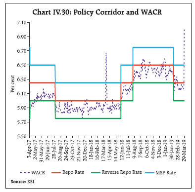
| Table IV.7: WACR, Repo and Net LAF | | Months | WACR < Repo Rate | WACR > Repo Rate | Average net LAF deficit (-) /surplus (+) | | | Number of days* | (₹ billion) | | April | 18 | 1 | 496 | | May | 22 | 0 | 142 | | June | 20 | 1 | 140 | | July | 22 | 0 | -107 | | August | 20 | 0 | 30 | | September | 11 | 7 | -406 | | October | 15 | 6 | -560 | | November | 18 | 0 | -806 | | December | 12 | 8 | -996 | | January | 23 | 0 | -329 | | February | 8 | 11 | -687 | | March | 18 | 1 | -570 | *: Working days excluding Saturdays.
Source: RBI. |
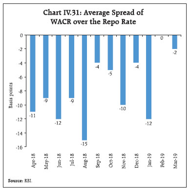 In view of the increased liquidity demand every year in March due to a variety of year-end factors, the Reserve Bank decided to conduct four longer term variable rate repo auctions (tenor ranging between 14-day and 56-day) during the month in addition to the regular 14-day variable rate term repo auctions. Furthermore, the Reserve Bank decided to augment its liquidity management toolkit and inject rupee liquidity for longer duration through long-term foreign exchange buy/sell swaps. Accordingly, it conducted a US$/₹ buy/sell swap auction of US$ 5 billion for tenor of 3 years on March 26, 2019, to inject durable liquidity of ₹345.6 billion into the system. Furthermore, the Reserve Bank announced another buy/sell swap auction of US$ 5 billion for tenor of 3 years to be conducted on April 23, 2019. IV.4 Conclusion Domestic financial markets continued to be influenced by global developments, especially volatile capital flows. The direction of capital flows remains unpredictable, posing challenges for macroeconomic and liquidity management. The exuberance in the equity market in H1:2018-19 generally continued in H2:2018-19, barring some bearishness in October, January and February. Credit growth has been healthy, notwithstanding some deceleration in recent months. Going forward, liquidity operations would continue to focus on achieving the stated policy objective of aligning the WACR with the policy repo rate by meeting the durable liquidity needs of the economy. Adequate and swift monetary transmission remains a policy challenge for the Reserve Bank.
_____________________________________________________________________________
V. External Environment Global growth has lost pace led by deceleration in major advanced economies (AEs) and emerging market economies (EMEs). Ongoing trade tensions have clouded the world trade outlook. Inflation pressures across geographies have remained muted. Financial markets, which ended 2018 on a volatile note, witnessed revival of risk-on sentiment in Q1:2019 on accommodative policy stances and benign oil prices. Since the MPR of October 2018, increasing apprehensions over a sharper than anticipated growth slowdown in the US, China and the Euro area have risen on incoming macroeconomic and financial data. Announcements of policy stimulus by China and accommodative monetary policy stances adopted by key central banks have provided some relief, along with hopes of a positive outcome from the US-China trade negotiations. Global financial markets ended 2018 on a volatile note, after a steep sell-off in risk assets. Risk-on sentiment revitalised in Q1:2019 on accommodative policy stances and benign oil prices even as the demand for safe haven assets has remained resilient in the face of the possibility of a hard/no-deal Brexit and geo-political challenges. V.1 Global Economic Conditions Among the major AEs, the US economy slowed during Q4:2018, pulled down mainly by private consumption as reflected in slowing retail sales. The slowdown appears to have continued in Q1:2019. The US manufacturing purchasing managers’ index (PMI) fell further in March 2019, pointing to the slowest growth in factory activity since June 2017 amidst weak demand, rising uncertainty across manufacturing supply chains, and an uncertain global trade outlook (Table V.1). Consumer sentiment, however, improved in Q1 on favourable real income expectations and the statement by the US Fed that it would be patient in future adjustments in the policy rate. The Euro area economy ended 2018 on a tepid note due to muted industrial activity and soft domestic demand. Among its key constituent economies, while Germany managed to register flat growth, Italy entered into technical recession (contraction in GDP growth for two consecutive quarters) in Q4:2018. The slowdown in the Euro area has carried over into Q1:2019. The manufacturing PMI slipped further into contraction in Q1 on falling export orders. The outlook remains clouded by tariffs on the automobile sector and uncertainty surrounding the Brexit. The Japanese economy returned to growth in Q4:2018, after contracting in Q3, on the back of a rebound in household consumption and business investment. However, the latest data on manufacturing activity and retail sales suggest that growth has lost momentum in Q1. Economic activity is expected to continue its moderate expansion in 2019, supported by an accommodative monetary policy stance and frontloaded consumer spending ahead of a planned sales tax hike. | Table V.1: Real GDP Growth (q-o-q, annualised) | | (Per cent) | | Country | Q4-2017 | Q1-2018 | Q2-2018 | Q3-2018 | Q4-2018 | 2019 (P) | 2020 (P) | | Advanced Economies | | Canada | 1.7 | 1.3 | 2.6 | 2.0 | 0.4 | 1.9 | 1.9 | | Euro area | 2.8 | 1.6 | 1.6 | 0.4 | 0.8 | 1.6 | 1.7 | | Japan | 1.6 | -0.4 | 1.9 | -2.4 | 1.9 | 1.1 | 0.5 | | South Korea | -0.8 | 4.0 | 2.4 | 2.4 | 4.0 | 2.6 | 2.8 | | UK | 1.6 | 0.4 | 1.6 | 2.8 | 0.8 | 1.5 | 1.6 | | US | 2.3 | 2.2 | 4.2 | 3.4 | 2.2 | 2.5 | 1.8 | | Emerging Market Economies | | Brazil | 1.2 | 1.6 | 0.0 | 2.0 | 0.4 | 2.5 | 2.2 | | China | 6.4 | 6.0 | 6.8 | 6.4 | 6.0 | 6.2 | 6.2 | | Malaysia | 4.0 | 5.6 | 1.2 | 6.4 | 5.6 | 4.6 | 4.8 | | Mexico | 4.2 | 4.1 | -0.6 | 2.4 | 1.0 | 2.1 | 2.2 | | Russia* | 0.9 | 1.9 | 2.2 | 2.2 | 2.7 | 1.6 | 1.7 | | South Africa | 3.4 | -2.7 | -0.5 | 2.6 | 1.4 | 1.4 | 1.7 | | Thailand | 1.2 | 8.3 | 4.4 | -1.3 | 3.3 | 3.9 | 3.7 | | Memo: | 2018 (E) | 2019 (P) | 2020 (P) | | World Output | 3.7 | 3.5 | 3.6 | | World Trade Volume | 4.0 | 4.0 | 4.0 | E: Estimate P: Projection *: y-o-y growth
Sources: Bloomberg; and International Monetary Fund. | Economic activity slowed in some major EMEs in Q4:2018 on the back of slowing industrial activity resulting from subdued global demand. The Chinese economy decelerated in Q4 on subdued domestic and global demand impacting industrial activity. Retail sales lost steam due to financial deleveraging and slowing global growth. Incoming data suggest that much of this weakness in economic activity extended into Q1:2019 as manufacturing activity remained subdued with factory output growth of 5.3 per cent in January-February turning out to be the weakest reading since the data series began in 1995. Fiscal stimulus and easing liquidity conditions, however, could buttress domestic demand, going forward. In Russia, incoming data suggest that the economy was showing some signs of recovery in Q1 as reflected by the uptick in retail sales and industrial production. South Africa emerged from recession in Q3:2018, though industrial production ended 2018 on a soft patch and retail sales contracted in December 2018. Economic recovery in Brazil was proceeding at a slower pace than earlier envisaged amidst positive political developments and pension reforms. During Q1:2019, incoming data suggests that economic activity remained weak on both domestic and external headwinds. Elsewhere in Asia, economic activity remained somewhat mixed. In Thailand, growth recovered during Q4:2018 from a contraction in the previous quarter, although subdued retail sales and weak industrial activity remained soft spots. Growth recuperated in Malaysia in Q4 as slowing inflation boosted consumption. The Indonesian economy lost pace in Q4 with retail sales falling and exports slumping. The Turkish economy entered into recession in Q4:2018 after a tumultuous year – a currency crisis amidst a challenging political situation. The outlook for the economy remains uncertain as inflation, though falling, remains well above the target. The global composite PMI registered a mild gain in February – after declining to 28-month low in January – on improved growth in services (Chart V.1a). Among the major OECD economies, composite leading indicators (CLIs) suggest slowing of growth momentum in major AEs and EMEs in Q4:2018, barring Brazil (Chart V.1b). 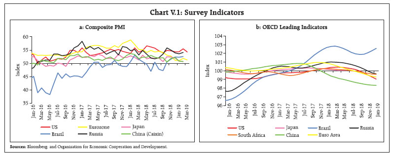 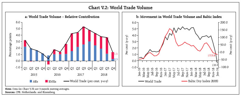 Global trade growth slowed down in Q4:2018, though an increase in commodity prices partly offset the deceleration in volumes. AEs and EMEs have both been impacted by the slowdown in trade, though the loss of momentum is somewhat higher for EMEs (Chart V.2a). In line with recent trends, forward looking indicators suggest that world trade is likely to slow down further in 2019. The World Trade Outlook Indicator (WTOI)1 has slipped below trend, following a slowdown in the past four quarters. All major components such as export orders, international air freight and automobile production have suffered loss of momentum. Movement in other indicators such as the Baltic Dry Index also suggests a moderation in global trade (Chart V.2b), with ongoing trade tensions clouding the outlook. V.2 Commodity Prices and Inflation Global commodity prices have been largely driven by demand-supply factors, geo-political concerns and trade tensions. The Bloomberg commodity index declined by 6.1 per cent between October 2018 and March 2019. The food price index of the Food and Agriculture Organisation (FAO) increased by 2.8 per cent between October 2018 and February 2019. Global food prices declined in November 2018 to their lowest levels in more than two years. They, however, firmed up in Q1, buoyed by prices of many food items, especially dairy products, due to tightening export supplies on account of a seasonal decline in production and robust import demand. Rising international sugar prices due to concerns over production prospects and appreciation of the Brazilian real also added to the rise in the food price index (Chart V.3a). Brent crude price declined sharply by 20.7 per cent between October 2018 and March 2019 on mounting oil inventories in the US and on the back of slowing global demand. Crude prices recovered somewhat from their December lows in Q1:2019 (Chart V.3b). The outlook for crude oil prices, however, remains uncertain (Box V.1). Base metal prices, measured by the Bloomberg base metal spot index, increased by 3.2 per cent between October 2018 and March 2019. Base metal prices witnessed selling pressures in Q4:2018 on global trade uncertainty, but recovered most of the losses in Q1:2019 on supply disruptions and expectations of positive outcome from trade negotiations. Copper prices seemed to be firming up on concerns over tighter supply and increasing demand, after remaining low in Q4:2018 due to trade tensions and slowing of the Chinese economy. Gold prices continued to rise due to safe-haven demand, with intermittent falls in February on a stronger dollar and news on positive developments of the China-US trade deal. It recovered some of its losses subsequently on weak global economic outlook and accommodative policy stances by central banks (Chart V.4). 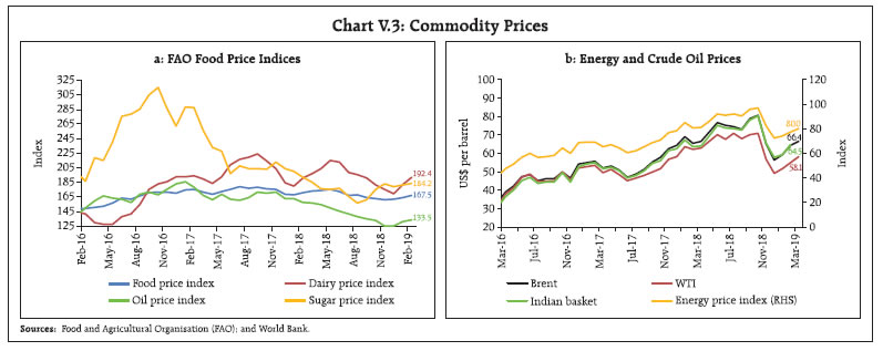
Box V.1: Crude Oil Prices – Near-term Outlook Global crude oil price movements have been volatile in 2018 and 2019 so far. Brent crude oil price, which was at around US$ 69 per barrel in January 2018, moved up to around US$ 80 per barrel by October 2018 before collapsing to US$ 56 per barrel in December 2018. It recovered to around US$ 68 per barrel by end-March 2019 (Chart V.1.1). 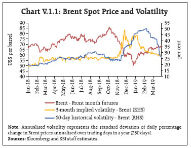 With robust global demand and OPEC plus2 countries’ production cuts in force, crude oil inventories slipped below their long-term averages from early 2018 onwards, leading to a sharp upturn in international crude oil prices to above US$ 80 per barrel in October. Speculative interest in crude also increased significantly during this period. Thereafter, in a matter of two months beginning mid-October, all the gains in prices between October 2017 and mid-October 2018 were reversed under the combined impact of record US shale oil production, OPEC over-production during the latter part of 2018 and significant slowdown in global demand, tilting the global oil balance to oversupply. Reflecting these developments, a sharp backwardation3 in the futures market for crude oil which was seen at the beginning of 2018 shifted to contango4 during November-December 2018. This was coupled with heightened implied and historical volatility of crude oil prices (Chart V.1.1). With the reduction in OPEC crude oil supplies in line with the Vienna agreement of December 20185, prices reversed in 2019 in anticipation of a tight oil market, thereby also switching oil futures markets back to backwardation, as seen in the front-end positive spreads for Brent futures (Chart V.1.2). As crude prices started to pick up, implied volatility in crude oil markets has shown a substantial moderation since mid-January 2019. 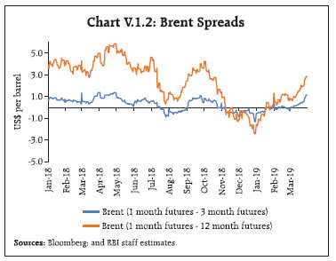 Historically, the prices of crude oil have been influenced mainly by three factors, viz., (i) the demand-supply balance; (ii) crude oil inventory levels; and (iii) the speculative interest in crude oil (Hamilton, 2008; Juvenal and Petrella, 2015). This is corroborated by an analysis on determinants of Brent prices based on monthly data from January 2011 to February 2019. The following equations were estimated to identify the determinants of Brent crude oil prices: Where ΔP is the annualised per cent change in Brent crude oil price; ΔI is the annualised per cent change in global inventory; NS is net supply (global crude oil supply – global crude oil demand); Spec is the annualised per cent change in net long speculative positions in Brent market; pmi is the US Manufacturing Purchasing Managers’ Index representing global aggregate demand; SpecExit = -1* Spec*D; SpecEntry = Spec *(1-D); where D=1, Spec if <0 and 0 otherwise. 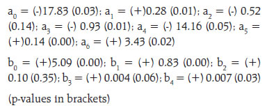 The empirical estimates suggest that any increase in global inventory tends to significantly reduce crude oil prices. As expected, the net supply balance also affects prices negatively. On the other hand, an increase in aggregate demand significantly increases crude oil prices. Further, any increase in speculative activity in the market also tends to increase prices. The volatility in Brent prices is determined by the quantum of speculative activity in markets. While both large exits and entries increase the variability in prices, the speculative entry has a larger impact on the volatility. Going into 2019, the key factor from the point of view of demand supply balance would be the staying power of the OPEC agreement on production cuts. Compliance with recent OPEC production cuts has been as high as 94 per cent6, with reports7 that OPEC is likely to extend production cuts well into 2019 in its meeting scheduled for April 2019. In addition to planned production cuts, the continuing worsening of geo-political tensions relating to Venezuela and sanctions on Iran’s exports have impacted the sour global crude oil supply. Going forward, the implementation of International Maritime Organization’s (IMO) 2020 global sulphur cap on shipping fuel would put additional pressure on sour grade crude oil. A combination of these factors is exerting pressure on global crude oil markets and is also resulting in a narrowing of price spreads between Brent and Dubai/Oman crude. The outlook on crude oil supply in the near-term would also be contingent on the rate of increase in US shale oil production. The outlook is one of the US becoming a net exporter of crude by 2021 driven by shale oil (IEA, 2019). In the near-term, however, there are signs of a slowdown in the rate of increase in shale oil rigs as investors have turned cautious and remain focused more on cash flows. As fresh investment awaits further cues on the direction of prices, some tempering of the shale oil momentum may be expected in the immediate term. 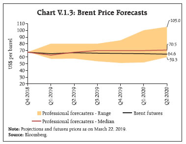 A significant factor impinging on the near-term outlook for crude oil prices is the global oil demand outlook. In 2019 so far, high frequency indicators suggest an increased appetite for commodities with energy indices generating the highest returns to date in 2019. The relationship between equity markets and commodities has also strengthened in the year so far8. Historically, the estimation results on determinants of crude oil prices show that increased financial interest in crude has significantly amplified the volatility in prices during times of large speculative interests and unwinding of such positions. Should there be a resolution of ongoing trade disputes, global demand prospects could brighten, leading to an uptick in crude oil prices. This, in turn, could result in sharp increases in net long speculative positions on crude futures, possibly further pulling up crude oil prices. On the other hand, concerns about the demand outlook, which has been rekindled with the inversion of the 10-year yield curve in the US9, could bring about sharp unwinding of long speculative positions, amplifying price declines. In a baseline case, a strong push by OPEC for higher prices, on the one hand, and the prospects of a massive response from shale oil producers, if prices pick up significantly on the other, may keep crude oil prices range-bound over the course of the year, as is also reflected in the professional forecasters’ median estimates and the futures curve (Chart V.1.3). References: Hamilton, J. D. (2008), “Understanding Crude Oil Prices”, NBER Working Paper No. 14492, November. International Energy Agency (2019), “Oil 2019: Analysis and Forecast to 2024”, March. Juvenal, L., and I. Petrella, (2015), “Speculation in the Oil Markets,” Journal of Applied Economics. 30, pp. 621–649. | Inflation edged lower in major AEs and many key EMEs. Among AEs, CPI inflation in the US has declined since November 2018, remaining below 2.0 per cent on account of a continuous fall in energy prices and weakening of economic activity. Core personal consumption expenditure (PCE) – the Fed’s preferred measure of inflation – moderated to 1.8 per cent (y-o-y) in January 2019 from 2.0 per cent in December and was expected to weaken further in Q1:2019 on increased pessimism about the near-term growth outlook. Inflation in the Euro area has fallen consistently since October 2018 on the back of falling energy prices and weak growth. In Japan, inflation eased to 0.2 per cent (y-o-y) in February 2019, pulled down by falling food, transport and housing prices (Chart V.5a). 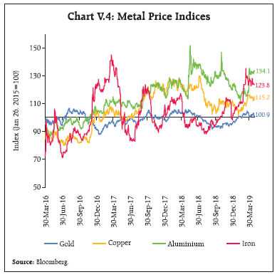 Inflationary pressures are easing in many EMEs (Chart V.5b). China’s consumer price inflation fell to 1.5 per cent in February 2019 due to subdued international and domestic demand on the back of lingering uncertainty over the US-China trade negotiations. In Brazil, inflation has fallen since October 2018 due to a sharp fall in oil prices and a cut in administered prices by the Government. However, inflation inched up slightly in February with increase in prices of food and non-alcoholic beverages. In South Africa, the inflation rate has eased in Q1 on falling energy prices. In Russia, inflation reached its highest level in two years in February at around 5 per cent due to increased value added tax and weaker rouble. In Indonesia, inflation remained below the target of 3.5 per cent through Q4:2018 to touch its lower bound in March due to deflation in administered prices. Inflation in Turkey has fallen consistently since October 2018 on ebbing domestic and global headwinds, along with a tight monetary policy stance. V.3 Monetary Policy Stance Monetary policy is increasingly becoming accommodative in most AEs and EMEs in the face of a slowing global economy and persisting US-China trade frictions. The US Fed left the policy rate unchanged at 2.25-2.50 per cent in its meetings in 2019 so far after raising it four times in 2018 and indicated that it would be patient in future rate adjustments (Chart V.6a). The European Central Bank (ECB) kept its key interest rates unchanged against the backdrop of growing downside risks to the economic outlook. In March 2019, the ECB announced targeted longer-term refinancing operations (TLTRO-III) starting in September 2019 and ending in March 2021, each with a maturity of two years, reflecting its concerns about the growth outlook, and indicated to maintain policy rates at low levels, at least through the end of 2019. The Bank of Japan (BoJ) continued with its highly accommodative monetary policy stance in Q1 as it cut its inflation forecasts in January 2019 on expectations of weakening economic activity due to a consumption tax hike to be implemented in October 2019. 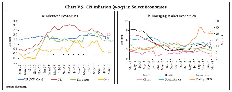  Monetary policy stances in many EMEs are also turning more accommodative with moderation in inflation pressures resulting from lower oil prices and weak demand. Among BRICS countries, the People’s Bank of China (PBOC) maintained its “prudent and neutral” policy stance and indicated more forward-looking, flexible and targeted policy reactions. In order to boost lending, the PBOC eased reserve requirements ratio and adjusted the assessment criteria of loans to small and medium enterprises in January 2019. Brazil kept its policy rate unchanged in February-March. Russia, after hiking its policy rate in December, left it unchanged in Q1:2019. South Africa kept its policy rate unchanged in Q1, after increasing it in November. Among other EMEs, Mexico raised its policy rate twice in Q4:2018 on rising inflation risks and uncertainty around economic policies by the new government. However, it kept its policy rate unchanged during Q1. Chile raised its policy rate twice during October-January, responding to the regained dynamism in economic activity. However, it kept the policy rate unchanged in its March meeting due to moderation of inflation. Indonesia kept its policy rate unchanged in Q1. The Philippines kept its policy rate unchanged on moderating growth and inflation expectations in Q1 (Chart V.6b). V.4 Global Financial Markets Financial markets, which had barely recovered from the impact of currency market pressures in EMEs in August 2018, were unsettled by a renewed bout of volatility as equities witnessed a sell-off in Q4:2018 on adverse macroeconomic and geopolitical developments. Investors faced several disconcerting developments in 2018, including strengthening of the US dollar, trade disputes and sanctions. The economic policy uncertainty index was also on an upswing during Q4 on hostile economic and political developments (Chart V.7). However, some of these headwinds ebbed and markets entered 2019 on a relatively calmer note as central banks signalled accommodation and expectations of a resolution of the China-US trade conflict gained traction. Global equity prices witnessed selling pressures during Q4:2018, with equity markets in both the advanced and emerging economies declining sharply due to a series of events such as spike in bond yields, triggered by Fed tightening, persistent trade frictions and political uncertainty in Europe. US stocks corrected in October, pulled down by the technology index despite better earnings due to the concerns over economic slowdown and trade tensions. Among other AEs, the narrative remained broadly unchanged as markets tumbled on political tensions in Europe surrounding Italy and Brexit. A fall in crude oil prices and rise in the US dollar also contributed adversely to the risk-off sentiment in November. The sell-off in global equity markets continued till the end of Q4, reflecting market reactions to the possibility of a US government shutdown and general discontent surrounding the direction of the Fed’s policy. However, reversing the situation, global equity markets recovered their losses during Q1:2019. Stocks in AEs registered impressive gains in January, rising by 7.7 per cent on improving outlook for US-China trade talks and an accommodative monetary policy stance by the Fed. Equity markets in the US strengthened, reversing most of December’s losses. European equities rose as global markets rallied, but enthusiasm was dulled by soft economic data, Brexit and Italy’s economic woes. Japanese equities firmed up in tandem with global equities, but mixed economic data and downgrade to the inflation outlook by the Bank of Japan weighed on investor sentiment and capped gains. Stock markets in the EMEs gained in Q1 driven by country-specific factors against the background of a less hostile global environment as key central banks paused policy rate hikes. In Brazil, stocks surged on improved business sentiment and announcement of pension reforms. Chinese equities gained on positive developments on trade talks and domestic stimulus. Russian equities increased on strong gains in crude oil and the rouble in Q1 (Chart V.8). 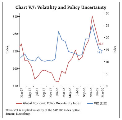 Bond yields edged lower during Q4:2018, reflecting increased risk aversion and volatility amidst uncertainty relating to trade tensions, Brexit and political concerns in Italy. In the US, 10-year Treasury yields fell on dovish comments by the Fed. In Europe, bond yields fell on soft economic data, though the ECB confirmed in its December meeting that it would end the bond purchase programme. Japanese bonds yields fell significantly on weak risk appetite triggered by growth concerns and entered into negative territory in December 2018. In the US, bond yields continued to decline in Q1:2019 due to weak economic data and central banks adopting a more cautionary language, while bond yields in Japan fell deeper into negative territory after a brief uptick in January. In the Euro area, bond yields slipped into negative territory in March. Emerging markets bond yields fell as Q4 progressed, with easing inflation pressures, weaker energy prices, and soft monetary policy stances (Chart V.9a). The US dollar strengthened during much of Q4:2018 on a tighter monetary policy stance by the Fed and strong economic data, though it ended the quarter on a soft note, falling in December 2018 on expectations of a softer Fed stance in 2019. Much of the US dollar’s weakness spilled into 2019 on the Fed’s dovish monetary policy stance and weak manufacturing data, though it ended Q1 on bullish note due to relatively better performance of the US economy vis-a-vis its peers. Persisting trade tensions, coupled with fears of a global growth slowdown, contributed to the strengthening of the Japanese yen, though it lost some ground in Q1:2019 on soft data and buoyant risk appetite. The euro fell against the US dollar in Q4 due to continued fragility in some of the member countries, aggravated by political tensions surrounding Italy and Brexit during November, but staged a mild comeback in December on the US dollar’s weakness. The euro failed to maintain the year-end momentum and witnessed selling pressures in Q1:2019 on fears of a broader slowdown in Europe. Most of the emerging market currencies emerged out of the downward pressure, experienced after the Turkish turmoil, trimming their past losses during the final quarter of 2018. They began 2019 on a bullish note as the Fed indicated an end to its rate normalisation cycle in conjunction with other positive events like soft crude prices, monetary easing by China and abating trade tensions, though it witnessed selling pressures in mid-February due to country-specific events and a weakening global growth outlook. Between October 2018 and March 2019, the JP Morgan emerging markets currency index increased by 0.5 per cent, though currencies are still trading below their levels witnessed in the summer of 2018 (Chart V.9b). V.5 Conclusion In sum, global economic activity is witnessing a synchronised deceleration, though easy policy stances by the fiscal and monetary authorities in several economies are expected to cushion the pace of the slowdown. The global trade outlook is uncertain as the largest economies of the world struggle to strike a deal. Inflation pressures across geographies remain benign on soft commodity prices and slowing demand. Global growth and trade concerns are expected to remain the dominant theme of 2019, which will drive markets and condition future monetary and fiscal actions.
_____________________________________________________________________________
ABBREVIATIONS | ADs | Authorised Dealers | | AEs | Advanced Economies | | AIC | Akaike Information Criteria | | AIFIs | All India Financial Institutions | | AL | Agricultural Labourers | | ARDL | Autoregressive Distributed Lag | | BE | Budget Estimates | | BK | Baxter-King | | BoJ | Bank of Japan | | bps | Basis Points | | BRICS | Brazil, Russia, India, China and South Africa | | CAD | Current Account Deficit | | CBLO | Collateralised Borrowing and Lending Obligation | | CCIL | Clearing Corporation of India Ltd. | | CD | Certificate of Deposit | | CDS | Credit Default Swap | | CF | Christiano-Fitzgerald | | CiC | Currency in Circulation | | CI | Confidence Interval | | CII | Confederation of Indian Industry | | CLI | Composite Leading Indicator | | CMB | Cash Management Bill | | CP | Commercial Paper | | CPC | Central Pay Commission | | CPI | Consumer Price Index | | CPI-AL | Consumer Price Index for Agricultural Labourers | | CPI-IW | Consumer Price Index for Industrial Workers | | CPI-RL | Consumer Price Index for Rural Labourers | | CSO | Central Statistics Office | | CU | Capacity Utilisation | | CU (SA) | Capacity Utilisation (Seasonally Adjusted) | | DEA | Digestive Enzymes and Antacids | | DGCA | Directorate General of Civil Aviation | | DGCI&S | Directorate General of Commercial Intelligence and Statistics | | DISCOMs | Distribution Companies | | DSGE | Dynamic Stochastic General Equilibrium | | ECB | European Central Bank | | ECBs | External Commercial Borrowings | | EMDEs | Emerging Market and Developing Economies | | EMEs | Emerging Market Economies | | EU | European Union | | FAE | First Advance Estimates | | FALLCR | Facility to Avail Liquidity for Liquidity Coverage Ratio | | FAO | Food and Agriculture Organisation | | FBIL | Financial Benchmarks India Pvt. Ltd | | FCCBs | Foreign Currency Convertible Bonds | | FDI | Foreign Direct Investment | | FICCI | Federation of Indian Chambers of Commerce and Industry | | FIT | Flexible Inflation Targeting | | FNOG | Finance Neutral Output Gap | | FIMMDA | Fixed Income Money Markets and Derivatives Association | | FPI | Foreign Portfolio Investment/ Investor | | FRE | First Revised Estimates | | FX | Foreign Exchange | | FY | Financial Year | | GDP | Gross Domestic Product | | GFC | Global Financial Crisis | | GFCE | Government Final Consumption Expenditure | | GFCF | Gross Fixed Capital Formation | | GFD | Gross Fiscal Deficit | | GIC | General Insurance Corporation | | GIC HFL | GIC Housing Finance Limited | | GNDI | Gross National Disposable Income | | GSDP | Gross State Domestic Product | | G-Secs/GS | Government Securities | | GST | Goods and Services Tax | | GSTN | Goods and Services Tax Network | | GVA | Gross Value Added | | H1 | First Half of the Year | | H2 | Second Half of the Year | | HDFC | Housing Development Finance Corporation | | HFC | Housing Finance Company | | HP | Hodrick-Prescott | | HRA | House Rent Allowance | | IBC | Insolvency and Bankruptcy Code | | IEA | International Energy Agency | | IIP | Index of Industrial Production | | IL&FS | Infrastructure Leasing and Financial Services Limited | | IMF | International Monetary Fund | | INR | Indian Rupee | | IOCL | Indian Oil Corporation Limited | | IOS | Industrial Outlook Survey | | IT | Information Technology | | IMO | International Maritime Organisation | | LAF | Liquidity Adjustment Facility | | LCR | Liquidity Coverage Ratio | | LIBOR | London Inter-bank Offered Rate | | LIC | Life Insurance Corporation of India | | LIC HFL | LIC Housing Finance Limited | | LPA | Long Period Average | | LPG | Liquefied Petroleum Gas | | MAE | Mean Absolute Error | | Mb/d | Million Barrels per Day | | MCLR | Marginal Cost of Funds Based Lending Rate | | ME | Mean Error | | MFs | Mutual Funds | | m-o-m | Month-on-Month | | MPC | Monetary Policy Committee | | MPR | Monetary Policy Report | | MSF | Marginal Standing Facility | | MSME | Micro, Small and Medium Enterprises | | MSP | Minimum Support Price | | MVKF | Multivariate Kalman Filter | | NBFCs | Non-Banking Financial Companies | | NBFC-ND-SI | Systemically Important Non-deposit Taking Non-Banking Financial Company | | NCAER | National Council of Applied Economic Research | | NDTL | Net Demand and Time Liabilities | | NEER | Nominal Effective Exchange Rate | | NFC | Non-Food Credit | | NGDP | Nominal Gross Domestic Product | | NGNF | Non-Government Non-Financial | | NHB | National Housing Bank | | NPA | Non-Performing Asset | | NIIP | Net International Investment Position | | NOAA | National Oceanic and Atmospheric Administration | | NSDL | National Securities Depository Limited | | NSE | National Stock Exchange | | OD | Overdraft | | OECD | Organisation for Economic Co-operation and Development | | OG | Output Gap | | OMCs | Oil Marketing Companies | | OMOs | Open Market Operations | | OPEC | Organisation of the Petroleum Exporting Countries | | PADO | Public Administration, Defence and Other Services | | PBOC | People’s Bank of China | | PCA | Prompt Corrective Action | | PCE | Personal Consumption Expenditure | | PD | Primary Dealer | | PFCE | Private Final Consumption Expenditure | | PMI | Purchasing Managers’ Index | | PMKSY | PM Kisan Samman Yojana | | POL | Petroleum, Oil and Lubricants | | PSBs | Public Sector Banks | | PSU | Public Sector Undertaking | | Q1 | First Quarter | | Q2 | Second Quarter | | Q3 | Third Quarter | | Q4 | Fourth Quarter | | q-o-q | Quarter-on-Quarter | | QPM | Quarterly Projection Model | | RBD | Refined, Bleached and Deodorised | | RBI | Reserve Bank of India | | RE | Revenue Expenditure/Revised Estimate | | REER | Real Effective Exchange Rate | | RHS | Right Hand Side | | RL | Rural Labourers | | RMSE | Root Mean Squared Error | | RTGS | Real Time Gross Settlement | | SAAR | Seasonally Adjusted Annualised Rate | | SAE | Second Advance Estimates | | SCBs | Scheduled Commercial Banks | | SDLs | State Development Loans | | SEBI | Securities and Exchange Board of India | | SEM | Structural Macroeconometric Model | | SIAM | Society of Indian Automobile Manufacturers | | SLR | Statutory Liquidity Ratio | | SVAR | Structural Vector Autoregression | | T-Bill | Treasury Bill | | TLTRO | Targeted Longer-term Refinancing Operations | | UCM | Unobserved Components Model | | UDAY | Ujwal DISCOM Assurance Yojana | | UK | United Kingdom | | US | United States | | VAR | Vector Autoregression | | VIX | S&P 500 Volatility Index | | WACR | Weighted Average Call Money Rate | | WADTDR | Weighted Average Domestic Term Deposit Rate | | WALR | Weighted Average Lending Rate | | WMA | Ways and Means Advances | | WPI | Wholesale Price Index | | WTI | West Texas Intermediate | | WTO | World Trade Organisation | | WTOI | World Trade Outlook Indicator | | y-o-y | Year-on-Year | | YTM | Yield to Maturity | |