Against the backdrop of fundamental shifts in the operating procedure of monetary policy and market reforms undertaken over the last decade, a review of the liquidity developments during 2018-19 shows that there was smooth transmission of policy repo rate changes in the inter-bank call money market. Empirical findings highlight the importance of both rate and quantum channels in policy transmission at the short-end of the financial market spectrum. Introduction Liquidity management by central banks typically refers to the operating framework of monetary policy that ensures the first leg of transmission by anchoring an interest rate prevailing at the short end of the market spectrum – the operating target – to the policy interest rate. The framework comprises forward-looking assessment of liquidity conditions, effective communication with markets, appropriate choice of instrument/s and conduct of liquidity operations consistent with the stance of monetary policy. Even though liquidity management has short-term effects in financial markets, its implications are enduring in terms of its impact on consumption, investment and capital formation in the economy. It is from this standpoint that a central bank’s liquidity management strategy links the daily monetary policy operations, through the operating target, to overall macroeconomic developments by influencing the term structure of interest rates (Bindseil, 2004). Efficient liquidity management is critical to the operationalisation of monetary policy, the “plumbing in its architecture” (Patra, et al, 2016). The main challenge before liquidity management is to ensure swift and seamless transmission of changes in the policy instrument to the operating target on a continuous basis. Accordingly, central banks simultaneously modulate liquidity conditions by influencing supply conditions in the market for bank reserves, typically the inter-bank market. The efficacy of liquidity management operations hinges on being prescient in assessing liquidity and market conditions and deploying instruments productively, singly and/or in combinations. In turn, these operations ensure controllability of reserves, the integrity and smooth functioning of the payment and settlement architecture and the orderly evolution of the interest rate structure. The liquidity management framework of the Reserve Bank of India (RBI) has evolved through progressive refinements since 1999 in response to changing domestic and global conditions. Since 2011, the fixed overnight repurchase (repo) rate under the Liquidity Adjustment Facility (LAF) has been formally announced as the single monetary policy rate with the weighted average call money rate (WACR) as the operating target of monetary policy (RBI, 2011). The objective of liquidity management is to align the WACR with the policy rate. The legitimacy of this framework along with the full institutional architecture, accountability mechanisms, and communication requirements were laid out in the monetary policy framework agreement (MPFA) between the RBI and the Government of India (GoI) under the provision of the RBI Act amended in 2016 that inter alia set a medium-term inflation target of 4 ± 2 per cent for the RBI in February 2015 (Patra, 2017). The MPFA enjoins the RBI to set out the operating procedure on liquidity management framework and any changes effected therein from time to time in the public domain. This requirement is fulfilled through the Monetary Policy Report (MPR). This article addresses the trials and tribulations confronting the RBI during 2018-19 when domestic liquidity conditions witnessed large and dramatic swings between surplus and deficits in a setting characterised by the gradual normalisation of the US monetary policy, firming up of global interest rates, oscillating geo-political developments, trade tensions and volatile movements in international crude oil prices. In doing so, it seeks to undertake an analytical assessment of the performance of the RBI in achieving the objectives of liquidity management. An important aspect of this assessment is the management of durable liquidity engendered by large foreign exchange interventions in the context of heighted turbulence in currencies across emerging market economies (EMEs) and unusual surges in the demand for domestic currency. The rest of the article is organised into four sections. The current liquidity management framework is reviewed in Section 2. Developments during the year and outcomes vis-à-vis mandate are discussed in Section 3. An empirical evaluation of the transmission of policy impulses to the operating target is taken up in Section 4. The final section presents concluding observations. 2. Evolution of Liquidity Management Framework In consonance with the changing monetary policy framework in India, the operating procedure of monetary policy has undergone significant refinements. In April 1999, an Interim Liquidity Adjustment Facility (ILAF), operated through repos and lending against collateral of Government of India (GoI) securities, was introduced under which liquidity was injected at various interest rates, but absorbed at the fixed (reverse) repo rate. A collateralised lending facility (CLF) was established alongside an additional collateralised lending facility (ACLF), with export credit refinance and liquidity support to Primary Dealers (PDs) all linked to the Bank Rate. The transition from ILAF to a full-fledged liquidity adjustment facility (LAF) commenced in June 2000. With the introduction of the LAF, steering overnight money market rates emerged as the key challenge in daily liquidity management operations. The LAF was operated through overnight fixed rate repo (liquidity injection rate) and reverse repo (liquidity absorption rate) from October 2004 to guide the evolution of the term structure of interest rates, consistent with monetary policy objectives (Patra and Kapur, 2012). The LAF became the principal instrument of liquidity management, as it set up an interest rate corridor (with repo rate as the ceiling and reverse repo rate as the floor) varying between 100 bps and 300 bps. As an additional instrument, the Market Stabilisation Scheme (MSS) was introduced in April 2004 to relieve the LAF from the burden of sterilisation operations (Mohan, 2006). In the ensuing years, the operative policy rate alternated between repo and reverse repo rates depending on deficit and surplus liquidity conditions in the money market which were, in turn, influenced by dramatic swings in capital inflows/outflows. Such oscillating liquidity conditions resulted in call money rate exhibiting highly volatile movements, often breaching either the ceiling or the floor of the corridor. Accordingly, the operating framework was modified in May 2011. The repo rate was made the single independently varying policy rate for transmitting policy signals, on the premise of keeping the system in a deficit mode for efficient transmission of monetary policy impulses (RBI, 2011).1 A marginal standing facility (MSF) was instituted under which banks could borrow overnight at their discretion by dipping up to 1 per cent into the statutory liquidity ratio (SLR) at 100 basis points (bps) above the repo rate to provide a safety valve against unanticipated liquidity shocks (Patra et. al., 2016). The corridor was re-defined as a symmetric one with a fixed width of 200 bps. The repo rate was placed in the middle of the corridor while the reverse repo rate and the MSF rate were placed 100 bps below and 100 bps above the repo rate, respectively. Several shortcomings of this framework, however, came to the fore in the immediate aftermath of the global financial crisis and particularly, during the taper tantrum of May 2013. The Report of the Expert Committee to Revise and Strengthen the Monetary Policy Framework (Chairman: Dr. Urjit R. Patel; RBI, 2014) noted that excessive reliance of the RBI on the overnight segment of the money market should be avoided by deemphasising overnight repos; instead, liquidity management operations should be conducted through term repos of different tenors. Accordingly, the Committee recommended design changes and refinements in the operating framework with flexibility in the use of instruments but consistent with the overall objectives of monetary policy. Some elements of the revised liquidity management framework were put in place in September 2014. The key change in the framework was doing away with unlimited accommodation of liquidity needs at the fixed LAF repo rate. Other important aspects of the revised framework included: (i) provision of the predominant portion of central bank liquidity through term repo auctions; (ii) introduction of fine-tuning operations through repo/reverse repo auctions of maturities varying from intra-day to 28 days with liquidity assessment undertaken on a continuous basis; (iii) phasing out export credit refinance; and (iv) progressive reduction in the statutory liquidity ratio (SLR). Thus, liquidity modulation became increasingly at the discretion of the RBI than in the earlier framework. The main liquidity provision instrument - the 14-day term repo - is synchronised with the reserve maintenance period which allows market participants to hold central bank liquidity for a relatively longer duration. This facilitates lending in the term money segment of the interbank market and is expected to develop market segments and benchmarks for term transactions. More importantly, term repos wean away market participants from their passive dependence on the RBI for cash/treasury management.2 The liquidity management framework was further fine-tuned in view of the shift of monetary policy stance to an accommodative mode in April 2016. The Reserve Bank also indicated that it would smoothen the supply of durable liquidity3 over the year using asset purchases and sales as per requirements. During 2017-18, liquidity management operations were principally aimed at modulating system liquidity from a surplus mode to a position closer to neutrality, consistent with the stance of monetary policy. Anticipating that surplus liquidity conditions may persist throughout the year, both on account of liquidity overhang and higher capital inflows, the Reserve Bank provided forward guidance on liquidity in April 2017 when it indicated it would (i) conduct variable rate reverse repo auctions with a preference for longer term tenors to absorb the remaining post-demonetisation liquidity surplus; (ii) issue Treasury Bills (T-Bills) and dated securities under the market stabilisation scheme (MSS) to modulate liquidity from other sources; (iii) issue cash management bills (CMBs) of appropriate tenors in accordance with the memorandum of understanding (MoU) with the Government of India (GoI) to manage enduring surpluses due to government operations; (iv) conduct open market operations (OMOs) to manage durable liquidity with a view to moving system level liquidity to neutrality; and (v) fine-tune variable rate reverse repo/repo operations to modulate day-to-day liquidity (RBI, 2018). Moreover, in consonance with the recommendation of the Expert Committee to Revise and Strengthen the Monetary Policy Framework (Chairman: Dr. Urjit R. Patel), the width of the policy rate corridor was narrowed from 100 bps in April 2016 to 50 bps in April 2017 in a symmetric manner. Accordingly, the reverse repo rate under the liquidity adjustment facility (LAF) was placed 25 bps below the policy repo rate, while the marginal standing facility (MSF) rate was placed 25 bps above the policy repo rate. As a result, volatility (standard deviation) in the call money market reduced from 0.19 in 2016-17 to 0.10 in 2017-18 even as the volume of the total overnight market remained broadly unchanged. Liquidity management operations during 2018-19 were further facilitated by several regulatory changes. Based on an assessment of financial market conditions, the RBI progressively increased Facility to Avail Liquidity for Liquidity Coverage Ratio (FALLCR) taking the total carve out from the statutory liquidity ratio (SLR) available to banks to 15.5 per cent of their net demand and time liabilities (NDTL) by December 20184. The increase in FALLCR supplemented the ability of individual banks to avail liquidity, if required, from the repo market against high-quality collateral, which, over time, would improve the distribution of liquidity in the financial system. Moreover, with a view to align the SLR with the LCR requirement, it was proposed in December 2018 to reduce the SLR by 25 basis points every calendar quarter – the first such reduction being effective from the quarter commencing January 2019 – until the SLR reaches 18 per cent of NDTL. Furthermore, forward guidance on OMO auctions through the release of an advance schedule indicating the quantum of operations planned for the month helped in conditioning market expectations. Against the backdrop of these significant changes in the liquidity management framework, it is pertinent to analyse the developments during 2018-19 (April-December) in the next Section. 3. Liquidity Developments During 2018-19 a. Drivers and management of liquidity Reflecting domestic and global financial market conditions, systemic liquidity underwent significant shifts in the first three quarters of 2018-19. Intensification of fears on global trade tensions and faster than anticipated normalisation of the US monetary policy resulted in capital outflows from the beginning of the year exerting depreciation pressure on the domestic currency. Consequently, the RBI had to intervene through sale of foreign assets, which sucked out domestic liquidity (Annex Table 1). Large currency expansion, representing leakage of liquidity from the financial system, has been a feature persisting through 2018-19, exacerbating the pressure on system level liquidity. Around Diwali (November 7, 2018), for instance, weekly expansion in currency in circulation (CiC) of ₹494 billion was unprecedented (Chart 1). 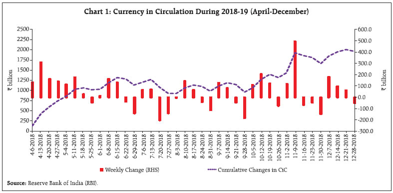 Given the significant changes in systemic liquidity across the first three quarters of 2018-19, it would be useful to introspect on the quarterly developments during the year. In Q1:2018-19, liquidity conditions generally remained in surplus, reflecting the Centres’ transfer of Goods and Services Tax (GST) proceeds to States in April and higher spending right up to June 2018. The resulting flow of liquidity into the system (₹1.4 trillion in April) more than offset the drain on liquidity caused by two autonomous factors5 – currency expansion by ₹743 billion and forex sales of ₹140 billion – during the month. The scale of forex sales picked up in May and June, and currency expansion continued to be higher than the usual seasonal upsurge, resulting in a liquidity deficit in the system for a brief period from mid-June to July 2018 (further exacerbated by advance tax outflows). Accordingly, the RBI injected liquidity through variable rate repo of various tenors, in addition to the regular 14-day repo, to tide over the liquidity tightness. In addition, two OMO purchases of ₹100 billion each were conducted by the RBI in May and June 2018 to infuse durable liquidity into the system (Chart 2). Overall, net liquidity absorption under the LAF moderated progressively during the quarter from an average daily net position of ₹496 billion in April to ₹140 billion in June. During Q2:2018-19, liquidity conditions gyrated. In July, moderation in government spending (especially in the second half) and the RBI’s forex sales, necessitated average daily net injection of ₹107 billion under the LAF, topped up with OMO purchases amounting to ₹100 billion during the month. The system moved back into absorption mode in August (up to August 19) due to increased spending by the Centre which even warranted recourse to ways and means advances (WMA) from the RBI, although indirect tax payments whittled down excess liquidity for a brief period. The RBI absorbed ₹30 billion on an average daily net basis during the month, even as systemic liquidity turned into deficit between August 20 and 30, necessitating liquidity injection. The system moved back into surplus during August 31 - September 10 as Government spending increased in the second half of the month, however, system liquidity swung back into deficit due to advance tax outflows. The RBI undertook daily net injection of liquidity through the LAF to the tune of ₹406 billion along with two OMO purchases amounting to ₹200 billion in the second half of September to meet durable liquidity requirements. Day to day systemic liquidity surplus was managed by the RBI through variable rate reverse repos auctions, with occasional and transient liquidity deficits met through regular 14-day variable rate term repos and other tenors (Chart 3). 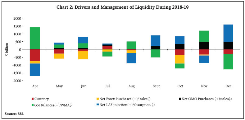 Liquidity conditions generally remained in deficit during Q3:2018-19. From the second week of October, the combination of stepped-up festival related large currency demand and the RBI’s forex sales resulted in a systemic deficit which continued for the rest of the month. With the Centre expanding spending including by resorting to WMA, the deficit moderated in the beginning of November, but increased subsequently as currency expansion was sustained during the festival season, and it increased in the second half of December mainly on the back of advance tax outflows. In order to meet liquidity needs, the RBI conducted variable rate repos auctions of various tenors, including longer term (28-day and 56-day) in addition to regular 14-day repos. Additionally, durable liquidity to the tune of ₹360 billion were injected through OMOs in October, which was subsequently scaled up to ₹500 billion each in November and December, thus taking the total durable liquidity injection to ₹1.36 trillion during the quarter (Table 1). RBI also conducted variable rate reverse repo auctions to mop up sporadic instances of excess liquidity. 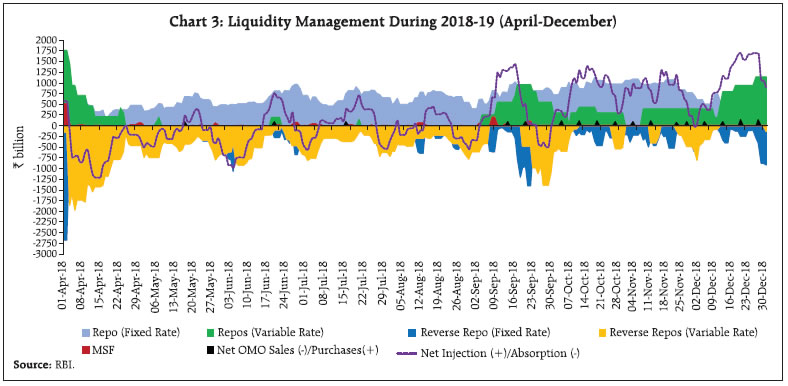
| Table 1: OMO Purchase Auctions During 2018-19 | | (April-December) | | (₹billion) | | Date of Auction | Amount | Month-wise | Quarter | | May 17, 2018 | 100 | May - 100 | | | June 21, 2018 | 100 | June - 100 | Q1 - 200 | | July 19, 2018 | 100 | July - 100 | | | September 19, 2018 | 100 | September - 200 | Q2 - 300 | | September 27, 2018 | 100 | | | | October 11, 2018 | 120 | | | | October 17, 2018 | 120 | October - 360 | | | October 25, 2018 | 120 | | | | November 01, 2018 | 100 | | | | November 06, 2018 | 100 | November - 500 | Q3 – 1,360 | | November 15, 2018 | 120 | | | | November 22, 2018 | 80 | | | | November 29, 2018 | 100 | | | | December 06, 2018 | 100 | | | | December 13, 2018 | 100 | December - 500 | | | December 20, 2018 | 150 | | | | December 27, 2018 | 150 | | | | Total (17 auctions) | 1,860 | 1,860 | 1,860 | | Source: RBI. | To summarise, the RBI’s forex operations and currency expansion turned out to be the prime drivers of durable liquidity in the banking system in 2018-19 whereas the ebb and flow of government spending was the key trigger for frictional liquidity movements. As a result, net LAF positions mirrored movements in government cash balances during the year (Chart 4). The unusual scale of the government’s spending through the availment of ways and means advances (WMA) and overdraft (OD) from June onwards, and the compensating variations in the net LAF positions is illustrative of the changing liquidity scenario during 2018-19 (Table 2). The temporary mismatches between receipts and payments of the government were met through recourse to CMBs on six instances aggregating ₹1.3 trillion during April – December. Large volumes of liquidity injections through longer term maturities (21, 28 and 56 days) were another defining feature of liquidity management during 2018-19, while reverse repos of 7 days maturity was the preferred instrument for absorbing liquidity in terms of frequency of usage - the relatively shorter maturity for absorption instruments perhaps signifying that episodes of surplus liquidity was not endemic (Table 3). | Table 2: Key Liquidity Indicators During 2018-19 | | (Number of days*) | | Month | Net LAF | GoI Cash Balances | | Deficit | Surplus | WMA/OD | Surplus | | April | 1 | 18 | 0 | 19 | | May | 5 | 17 | 4 | 18 | | June | 10 | 11 | 17 | 4 | | July | 16 | 6 | 16 | 6 | | August | 10 | 10 | 14 | 6 | | September | 12 | 6 | 9 | 9 | | October | 17 | 4 | 12 | 9 | | November | 18 | 0 | 14 | 4 | | December | 19 | 1 | 7 | 13 | *: Working days excluding Saturdays.
Source: Daily Press Release on Money Market Operations and RBI records. | The evolution of liquidity conditions and their management by the RBI gets encapsulated in the movement of bank reserves. The market for bank reserves evolves largely through the dynamic interaction between the central bank and depository institutions. If liquidity pressures from autonomous drivers of liquidity are not fully offset by liquidity management measures, it reflects in either drawdown or accumulation of bank reserves. An analytical scrutiny of the liquidity drivers and its management during 2018-19 (April-December) throws interesting insights. During the first quarter (April 1-June 29, 2018), autonomous drivers led to liquidity withdrawal more than what was injected through liquidity management operations; consequently, the deficit was met by large drawdown in bank reserves (Table 4). Large injection through repos under the LAF window along with OMO purchases significantly enhanced liquidity injection to the banking system during the third quarter, which reflected in accumulation of bank reserves. Thus, an aggregative picture of bank reserves (April-December) may be somewhat misleading in decoding liquidity movements during the year. 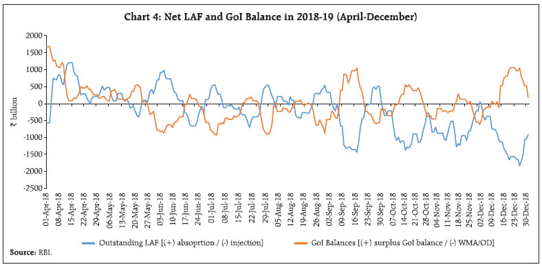
| Table 3: Fine-tuning Operations through Variable Rate Auctions (April-December) | | | Repo (maturity) | Reverse Repo (maturity) | | 7 | 8 | 14 | 21 | 28 | 56 | 2 | 3 | 4 | 6 | 7 | 11 | 13 | 14 | | Frequency (number of days) | 3 | 1 | 1 | 2 | 3 | 2 | 3 | 7 | 5 | 2 | 95 | 1 | 1 | 13 | | Average volume (₹ billion) | 165 | 250 | 142 | 325 | 250 | 225 | 456 | 344 | 249 | 186 | 140 | 41 | 26 | 44 | | Source: RBI. | b. Operating target and marksmanship The effectiveness of liquidity management lies in the precision with which the WACR – the operating target – can be aligned with the policy repo rate within the LAF corridor. During 2018-19 (April-December), the WACR generally remained below the repo rate while liquidity conditions oscillated between surplus and deficit conditions (Chart 5). A marked feature of the WACR’s movements was that it traded below the repo rate even after surplus conditions in the first quarter of 2018-19 ebbed and systemic liquidity was tight warranting net injection through repos (Table 5 and Chart 6). | Table 4: Liquidity and Bank Reserves ** | | {(+) Injection / (-) Absorption of liquidity from banking system} | | (₹billion) | | | April 1- Jun 29 | Jun 29-Sep 28 | Sep 28- Dec 28 | Total | | | (1) | (2) | (3) | 4 = (1+2+3) | | A. Autonomous Drivers of Liquidity (1+2+3+4) | -696 | -113 | -1915 | -2725 | | 1. Net Purchases from Authorised Dealers (ADs) # | -976 | -313 | -591 | -1881 | | 2. Currency in Circulation | -1138 | 179 | -997 | -1956 | | 3. Government of India Cash Balances | 1930 | -319 | -603 | 1007 | | 4. Others* | -512 | 340 | 276 | 104 | | B. Management of Liquidity (5+6+7+8) | 293 | 256 | 2195 | 2744 | | 5. Net Liquidity Adjustment Facility (LAF) @ | -259 | 90 | 1113 | 944 | | 6. Open Market Purchases | 207 | 300 | 1360 | 1867 | | 7. Standing Liquidity Facilities for Primary Dealers (PDs) | -1 | -5 | 2 | -4 | | 8. CRR Balances $ | 347 | -129 | -280 | -63 | | C. Bank Reserves (A+B) | -403 | 142 | 280 | 18 | ** : Calculations are based on data pertaining to last Friday of the month; first quarter variation is calculated over March 31, 2018.
# : Net OMO purchases include outright as also NDS-OM operations
* : include valuation changes, hair cut on operations, etc.
@ : Net LAF represents the liquidity position of fixed rate and variable rate repo and MSF net of reverse repo operations.
$ : Due to increase in NDTL (adjusted for change in excess CRR maintained by banks).
Source: RBI and authors calculations. |
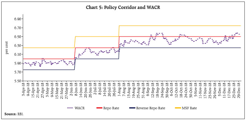 There are several reasons for this anomalous behavior: (i) most of the co-operative banks are not participants in the NDS-Call trading platform. Non-scheduled co-operative banks, District Central co-operative banks and State co-operative banks tend to enter the inter-bank call money market late in the trading hours - after the closure of the collateralised market segments – and their lending activity increases during the second half of the day thus driving rates below the repo rate; | Table 5: WACR, Repo and Net LAF | | Months | WACR < Repo Rate | WACR > Repo Rate | Average net LAF deficit (-) /surplus (+) | | | Number of days* | (₹ billion) | | April | 18 | 1 | 496 | | May | 22 | 0 | 142 | | June | 20 | 1 | 140 | | July | 22 | 0 | -107 | | August | 20 | 0 | 30 | | September | 11 | 7 | -406 | | October | 15 | 6 | -560 | | November | 18 | 0 | -806 | | December | 12 | 8 | -996 | *: Working days excluding Saturdays.
Source: RBI. | (ii) the first hour of trading in the inter-bank call money market usually accounts for about 75-80 per cent of the day’s volume as most of the market participants are unable to assess their inflows/outflows for the day in the absence of a robust liquidity forecasting framework, and as a result, late-hour demand supply mismatches reflect in low call rates; (iii) the absence of uniform market hours across all money market segments (including the collateralised segments), which are not in sync with real time gross settlement (RTGS) timings often have a destabilising impact on the WACR towards the market’s closure. 4. Policy Transmission - Empirical Evaluation We examine the factors determining movements in WACR by augmenting the empirical framework of Patra, et al. (2016) with suitable modifications. The explanatory variable, i.e., the change in WACR is explained by both the level and lagged changes in the WACR, the policy repo rate (RR), and outstanding balances under the net LAF as a proportion of net demand and time liability of scheduled commercial banks (RNLAF). While the impact of RR on the WACR represents the announcement effect of policy changes, the impact of the RNLAF on WACR captures the liquidity effect (Bhattacharyya and Sahoo, 2011). The empirical analysis is based on daily data covering the period January 1, 2014 – December 31, 2018. Unit root tests indicate that the null hypothesis of nonstationarity cannot be rejected for the WACR and RR. The same, however, is rejected for RNLAF. Bound tests reveal that the three variables (WACR, RR and RNLAF) are cointegrated. Therefore, it is appropriate to use the autoregressive distributed lag (ARDL) approach (Pesaran, et al., 2001) instead of differencing the data and losing valuable information / data series properties especially when they are of different orders of integration. The base line specification for capturing short-run dynamics is given below: 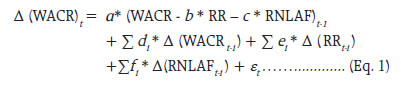 In the next step, we augment Eq.1 with dummies to capture market idiosyncratic factors. Call money rates tend to spike towards the quarter-end when banks generally reduce lending in the call money market in order to avoid higher risk weights on lending in the uncollateralised segment for meeting their capital adequacy requirements. This phenomenon is captured through an end-quarter dummy (D_quarter). Furthermore, maintenance of reserve requirements is subject to a daily end-of-the-day minimum and fortnightly averaging – i.e., banks hold excess reserves in the first week while drawing down during the second week of the fortnightly reserve maintenance period. The shortage of eligible collateral with liquidity deficient banks prevents access to the RBI’s standing facilities on some days of the reserve maintenance period, which can also lead to fluctuations in daily call rates. Accordingly, these effects are sought to be captured by daily dummies (D_daily - represented by dummies D2 to D10)6 in the baseline specification. Thus, the extended specification is: 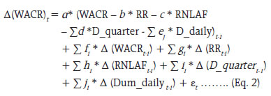 The estimates of the baseline and the augmented models are presented in Annex Table 2. As the results are qualitatively similar, we focus on the augmented specification (Model 3) for the narrative. The long-run coefficient of the policy repo rate is about unity indicating strong announcement effects, i.e., on an average, the call rate gets closely aligned to the policy rate ahead of liquidity modulating operations. At the same time, the liquidity effect is rather muted (a change of 100 bps in RNLAF results in a change of 7 bps in the WACR in the opposite direction), i.e., liquidity surplus (deficit) in the system leads to decline (increase) in the WACR. Moreover, the high value of the coefficient on D_quarter (positive and statistically significant) suggests significant pressure on the WACR at the end of each quarter. The coefficient of D_daily, however, turns out to be marginally positive (weakly significant) for the reporting fortnight. Finally, the short-run dynamics captured by the error correction term indicate that the speed of adjustment to any shock is significant – i.e., around 37 per cent of the deviation gets adjusted on the following trading day. The estimation results for a longer period sample (5 years) are at variance with the developments during the current year. In terms of the liquidity effect, the estimates point to a negative relationship between liquidity conditions and the WACR i.e., liquidity tightness (easing) should result in a hardening (softening) of the WACR above the repo rate. In sharp contrast, developments during the current year indicate that the WACR traded below the repo rate even when systemic liquidity was in deficit. This bears out our hypothesis of issues in market microstructure being at work - asynchronous market closure timings across segments; trading intensity high in early hours; and market timings not in sync with settlement timings. These factors merit greater attention in the ongoing efforts to improve transmission.7 5. Concluding Observations Liquidity management was subjected to conflicting pulls during 2018-19 in an environment suffused with global spillovers, the rapid pace of remonetisation and frictional high tides of budgetary spending. As a consequence, liquidity in the system underwent sizable churns that vitiated patterns of the recent past and necessitated atypical responses from the RBI in terms of the choice of instrument mix and the timing of deployment – for the first time, pre-announced OMO notified amounts entered the RBI’s arsenal of liquidity management instruments. Another defining feature of the 2018-19 experience is that liquidity absorption was conducted through short-tenor (4-7 days) reverse repo whereas liquidity injection was mainly through longer-tenor (28-56 days) repo, indicating that episodes of liquidity surplus in the system were transient. In the event, the combination of one-sided OMOs (purchases) and long-duration repo imparted a downward bias to the WACR which trailed below the policy rate throughout the year, warranting careful review of the framework’s performance in terms of the marksmanship objective that has been pursued with the progressive narrowing of the LAF corridor. The empirical results suggest that announcement effects tend to dominate over liquidity effects so that the market’s reactions to policy innovations are stronger and faster than the responsiveness of actual cost of funds to system liquidity shifts engendered by the policy changes when they fully play out. The results also underscore the need for assigning priority to reforms of the market microstructure if the full effects of the overhaul of the liquidity management framework are to be reaped in terms of marksmanship and efficiency of transmission. Significantly, however, the volatility of the WACR has reduced, stabilising market expectations. An unfinished agenda awaits the evolution of the liquidity framework. The 14-day repo, through which the bulk of primary liquidity is provided to satiate the demand for reserves, needs to replace the fixed rate overnight repo as the single policy rate. Two-way OMOs need to be conducted in a market-based framework so that quantity modulation occurs seamlessly rather than relying on announcement effects. The experience of 2018-19 also suggests that fine-tuning operations should be of short tenors and easily reversible, not overwhelming the durable liquidity operations. A more accurate assessment of liquidity needs is critical, combining top-down methodologies and bottom-up approaches. A roadmap for liquidity management reforms has been laid out (RBI, 2014), and it is apposite to carry its implementation forward. The success of liquidity management in terms of its objectives hinges around clear and transparent communication of intent, content, time frame and target(s). References Bindseil, U. (2004), “The Operational Target of Monetary Policy and the Rise and Fall of Reserve Position Doctrine”, Working Paper No. 372, European Central Bank. Bhattacharyya, I. and Sahoo, S. (2011) “Comparative Statics of Central Bank Liquidity Management: Some Insights,” Economics Research International, vol. 2011, Article ID 930672, available at https://doi.org/10.1155/2011/930672. Mitra, A.K., and Abhilasha, (2012), “Determinants of Liquidity and the Relationship between Liquidity and Money: A Primer”, RBI Working Paper, WPS (DEPR):14/2012. Mohan, R. (2006), “Coping with Liquidity Management in India: A Practitioner’s View”, Reserve Bank of India Bulletin, April. Patra, M. D., and Kapur, M. (2012), “A Monetary Policy Model for India”, Macroeconomics and Finance in Emerging Market Economies, 5(1), 16–39. Patra M.D., Kapur M., Kavediya R., and Lokare S.M. (2016), “Liquidity Management and Monetary Policy: From Corridor Play to Marksmanship”, in Ghate C., and Kletzer K. (eds) Monetary Policy in India, Springer, New Delhi, 257-296. Patra M.D. (2017), “One Year in the Life of India’s Monetary Policy Committee”, Reserve Bank of India Bulletin, December. Pesaran, M., Shin, Y., & Smith, R. (2001), “Bounds testing approaches to the analysis of level Relationships”, Journal of Applied Econometrics, 16, 289–326. Reserve Bank of India, (2011), “Report of the Working Group on Operating Procedure of Monetary Policy” (Chairman: Deepak Mohanty). Reserve Bank of India, (2014), “Expert Committee to Revise and Strengthen the Monetary Policy Framework” (Chairman: Dr. Urjit R Patel). Reserve Bank of India, (2016), “First Bi-monthly Monetary Policy Statement 2015-16”, April 5. Reserve Bank of India, (2018), “Annual Report 2017-18”, August.
Annex | Table 1: Movements in Key Drivers and its Impact on Systemic Liquidity | | Operation/Instrument/Variable | Change in (1) | Impact on Banking System Liquidity | | (1) | (2) | (3) | | Autonomous factors | | | | Currency in circulation | Increase | ↓ | | | Decrease | ↑ | | GoI Cash Balances | Build-up | ↓ | | | Drawdown | ↑ | | Forex intervention by RBI | Purchase | ↓ | | | Sales | ↑ | | Excess Reserves maintained by banks with RBI | Build-up | ↓ | | | Drawdown | ↑ | | Policy driven (Discretionary) factors | | | | Open Market Operations by RBI | Purchase | ↓ | | | Sales | ↑ | | Cash Reserve Requirements (CRR) | Increase | ↓ | | | Reduction | ↑ | | Net LAF position | Injection* | ↓ | | | Absorption# | ↑ | *: (Repos + MSF – Reverse Repos) > 0; #: (Repos + MSF – Reverse Repos) < 0; Increase (↑); Decrease (↓)
Source: Authors adaptation from Mitra and Abhilasha, 2014. |
| Table 2: Policy Rate, Liquidity and the WACR – Alternate Specifications | | Variables | Base Line - Model 1 | Augmented - Model 2 (with quarterly dummies) | Augmented - Model 3 (with both quarterly and daily dummies) | | Selected Modela | ARDL(5, 1, 1) | ARDL(5, 1, 1) | ARDL(5, 1, 1) | | Long-run equation: dependent variable: WACR | | | RR | 1.05 (0.00) | 1.06 (0.00) | 1.06 (0.00) | | RNLAF | -0.08 (0.00) | -0.07 (0.00) | -0.07 (0.00) | | D_quarter | - | 1.33 (0.00) | 1.32 (0.00) | | D_Daily10 | - | - | 0.03 (0.08) | | Error correction (-1) | -0.34 (0.00) | -0.37 (0.00) | -0.37(0.00) | | Adj. R2 | 0.94 | 0.95 | 0.95 | | F-Statistics | 37.75 | 50.51 | 50.81 | | Lower and upper bound critical value | 1% [4.13, 5.00] | 1% [4.13, 5.00] | 1% [4.13, 5.00] | | Q-statistics | 5.52 (0.85) | 21.99 (0.15) | 21.71 (0.17) | Note: Figures in parenthesis indicate p-value. aLag length is selected using Akaike Information Criteria (AIC).
Source: Author’s estimates. |
|