An analysis of the regional inflation dynamics in India reveals the presence of wide dispersion in inflation across states, largely driven by food price inflation. State level inflation tends to converge to the national average over time, however, validating the choice of national level consumer price inflation as the nominal anchor for monetary policy in India. Introduction With the adoption of a flexible inflation targeting (FIT) framework in India with consumer price inflation (all-India combined) as the numerical target, a path of disinflation has brought down inflation from 11.5 per cent in November 2013 to an average level of 3.6 per cent in 2017-18. This receding of inflation has not been even though, marked as it has been by seasonal surges, disruptive shocks including demonetisation, the Goods and Services Tax (GST), farmers’/transporters’ agitations, a deep downturn in food inflation on a combination of cyclical, irregular and policy-related forces and high volatility in international crude prices. As a result, inflation has generally eased across states, but with wide variations. For an inflation targeting (IT) central bank, regional heterogeneity in price movements could have a significant impact on the effectiveness of monetary policy. Large inflation differentials among regions within an economy can lead to significant variations in real interest rates and consequently, in levels of aggregate demand (Cecchetti et al, 2002; Beck et al, 2009). High dispersion of inflation across regions could also have implications for the labour markets in terms of wage rates and standards of living. Ignoring the regional dimensions of inflation may limit the effectiveness of a nationally set monetary policy in satisfying the needs of all regions equally (Beck and Weber, 2005; Weyerstrass et al, 2011). In the Indian context, ensuring that the benefits of low and stable inflation accrue across regions and states is critical for anchoring the credibility of the new monetary policy framework and for incentivising buy-in by the widest sections of society. Wide disparities across Indian states in terms of economic, geographic and structural factors warrant a careful examination of their role in regional inflation dispersion and hence on national inflation. Additionally, as the all-India consumer price index (CPI) is compiled as a weighted average of the state level price indices, i.e., a bottom-up approach, relative price movements across states will have a bearing on overall inflation outcomes. Accordingly, drilling down into the dynamics of regional inflation formation in India is the main motivation for this article. To briefly summarise, it finds that there is considerable regional dispersion, although largely influenced by supply side food price shocks. The estimated kernel density function as well as beta (β) convergence tests confirm that regional inflation tends to converge towards the national average inflation during the sample period. The remainder of the article is structured into five Sections. Section II provides a detailed analysis of inflation and its volatility at the national and regional levels as well as at aggregate and disaggregate levels to understand the pattern and driver of regional inflation dispersion in India. Section III draws on select contributions to the theoretical and empirical literature on regional inflation dynamics and monetary policy from a cross-country perspective. The convergence of inflation rates across states to the national inflation level is tested empirically in Section IV to examine whether an inflation target at the national level is appropriate. Section V provides concluding observations and policy implications. II. Some Stylised National/Regional Features Beginning in December 2013, headline CPI inflation1 has eased from an average of 10.0 per cent in 2012-13 to 3.6 per cent in 2017-18 and 4.2 per cent in the first seven months of the current fiscal year (April-October, 2018). Although a de jure flexible inflation targeting was established in September 2016, the path to its adoption was laid by de facto pre-commitments that initiated the disinflation and consolidated the gains accruing therefrom2 (Chart 1). In line with the all-India trend, inflation also moderated across states (Chart 2), albeit with wide variations relative to the former.
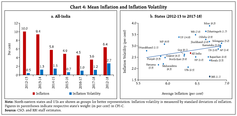
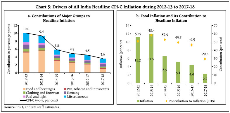
Notably, all the southern states had higher average inflation than northern states like Punjab, Haryana, Uttar Pradesh and Uttarakhand as well as states in other regions like Maharashtra and Madhya Pradesh. Bihar recorded the highest inflation of 16.1 per cent (November 2013), while Chhattisgarh recorded the lowest inflation level of (-) 2.3 per cent (June 2017) as against the national-level maximum of 11.5 per cent (November 2013) and minimum of 1.5 per cent (June 2017). Intra-year volatility (measured by the standard deviation of monthly year-on-year (y-o-y) inflation rates) varied considerably at both all-India and state levels (Chart 3). Generally, headline inflation volatility has increased, barring a blip in 2015-16, in spite of the moderation in mean inflation. A similar pattern is observed at the state level, with inflation volatility becoming more pronounced than at the national level, with states in the central and eastern regions experiencing higher inflation volatility than the other regions and at the all-India level (Table 1). Over this period, inflation and inflation volatility did not exhibit any noteworthy co-movement, which is in contrast with the two-way causality posited in the literature3. In fact, when inflation averaged a high of 10.0 per cent in 2012-13, its volatility was at the lowest in the period of study at 0.5 per cent; volatility rose to 1.2 per cent when average inflation was at its lowest level of 3.6 per cent in 2017-18 (Chart 4a). This relationship alters dramatically, however, in the regional setting. Unlike the all-India pattern, state-level inflation and inflation volatility co-moved during 2012-13 to 2017-18 (Chart 4b). Another interesting observation is that the states/regions that experienced high average inflation (e.g., Bihar, Chhattisgarh, Odisha and West Bengal) also recorded high volatility in inflation. At a disaggregated level, all-India headline inflation was driven largely by the movements in food inflation (Chart 5a). In fact, the sharp moderation in inflation during 2017-18 can be largely attributed to food inflation, with its contribution to overall inflation falling below 30 per cent from an average of 52 per cent in the previous five years (Chart 5b). Other major contributors were the miscellaneous group (which covers miscellaneous goods and services including petroleum products) and housing rentals. 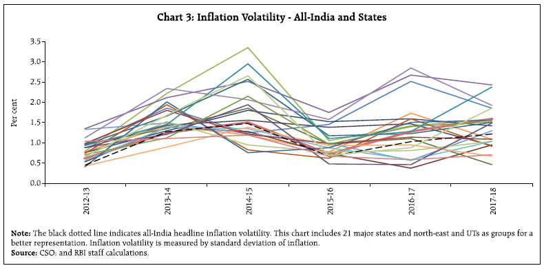
| Table 1: Regional CPI-C Inflation – Key Summary Statistics (2012-13 to 2017-18) | | | Weights in All India CPI | Mean | Maximum | Minimum | Standard Deviation | Skewness | Kurtosis | | Northern Region | 24.67 | 6.1 | 11.8 | 1.4 | 2.9 | 0.4 | -1.2 | | Haryana | 3.30 | 5.8 | 11.1 | 2.5 | 2.2 | 0.5 | -0.8 | | HP | 1.03 | 6.5 | 12.5 | 2.6 | 2.5 | 0.5 | -1.0 | | J&K | 1.14 | 6.7 | 10.6 | 3.2 | 1.7 | -0.2 | -0.2 | | Punjab | 3.31 | 5.9 | 11.0 | 2.1 | 2.6 | 0.4 | -1.1 | | UP | 14.83 | 6.2 | 12.2 | 0.4 | 3.4 | 0.3 | -1.2 | | Uttarakhand | 1.06 | 5.6 | 11.5 | 1.8 | 2.8 | 0.6 | -1.0 | | Western Region | 19.56 | 6.2 | 10.3 | 1.5 | 2.3 | 0.3 | -1.1 | | Gujarat | 4.5 | 6.0 | 10.8 | 0.2 | 2.5 | 0.1 | -0.8 | | Goa | 0.1 | 6.3 | 11.8 | 1.7 | 2.6 | 0.5 | -0.3 | | Maharashtra | 8.3 | 5.9 | 10.3 | 2.1 | 2.2 | 0.5 | -1.0 | | Rajasthan | 6.6 | 6.7 | 11.1 | 1.7 | 2.5 | 0.1 | -1.0 | | Central Region | 6.61 | 6.1 | 12.6 | -0.5 | 3.2 | 0.1 | -1.0 | | Chhattisgarh | 1.68 | 6.7 | 15.2 | -2.3 | 3.7 | -0.2 | -0.3 | | MP | 4.93 | 5.9 | 11.7 | 0.2 | 3.1 | 0.3 | -1.2 | | Eastern Region | 20.09 | 6.6 | 14.8 | 0.8 | 3.5 | 0.3 | -1.1 | | Bihar | 8.21 | 6.7 | 16.1 | 0.8 | 3.9 | 0.4 | -1.1 | | Jharkhand | 1.96 | 6.7 | 13.5 | 0.5 | 3.2 | 0.3 | -1.0 | | Odisha | 2.93 | 6.6 | 15.2 | -0.6 | 3.3 | -0.2 | -0.3 | | WB | 6.99 | 6.5 | 13.6 | 1.2 | 3.5 | 0.2 | -1.3 | | Southern Region | 24.70 | 6.8 | 11.5 | 2.0 | 2.6 | 0.4 | -1.0 | | Andhra Pradesh | 5.40 | 6.9 | 12.0 | 0.7 | 3.0 | -0.2 | -0.9 | | Karnataka | 5.09 | 6.9 | 12.8 | 1.5 | 3.0 | 0.2 | -0.9 | | Kerala | 5.50 | 6.7 | 11.1 | 2.9 | 2.4 | 0.3 | -1.0 | | Tamil Nadu | 5.55 | 6.9 | 11.9 | 1.5 | 2.9 | 0.4 | -0.9 | | Telangana | 3.16 | 6.9 | 13.8 | 1.6 | 3.1 | 0.7 | -0.7 | | North-eastern Region | 3.90 | 6.3 | 11.6 | 2.3 | 2.6 | 0.2 | -1.3 | | Of which, Assam | 2.63 | 6.1 | 11.7 | 1.2 | 3.0 | 0.0 | -1.4 | | Union Territories (UTs) | 0.5 | 6.3 | 10.8 | 3.0 | 2.1 | 0.5 | -0.9 | | All India | 100.00 | 6.4 | 11.5 | 1.5 | 2.7 | 0.3 | -1.2 | Note: North-eastern states and UTs are shown as groups for better representation.
Source: CSO; and RBI staff estimates. |
 Food inflation also exhibited the highest volatility (Chart 6), which, in turn, was transmitted to overall inflation, given the large weight of food (45.9 per cent) in the all-India CPI-C. At the sub-national level, there exists a positive relationship between average food inflation and overall inflation (Chart 7a). Similarly, a positive relationship between overall inflation volatility and food inflation volatility can be observed across states (Chart 7b). Overall, there seems to exist a strong co-movement between the inflation spread (measured as state headline inflation minus all-India headline inflation) and its volatility with the food inflation spread (measured as state food inflation minus all-India food inflation) and its volatility across states (Chart 8), with possible externalities for inflation expectations.
A simple panel regression4 covering all states with the food inflation spread as the explanatory variable and the headline inflation spread as the dependent variable while controlling for differences in income levels across states through gross state domestic product (GSDP) growth spread (measured as state GSDP growth minus all India GDP growth) reveals that 69 per cent of the variation in the inflation spread is explained by food inflation spread alone (Table 2). 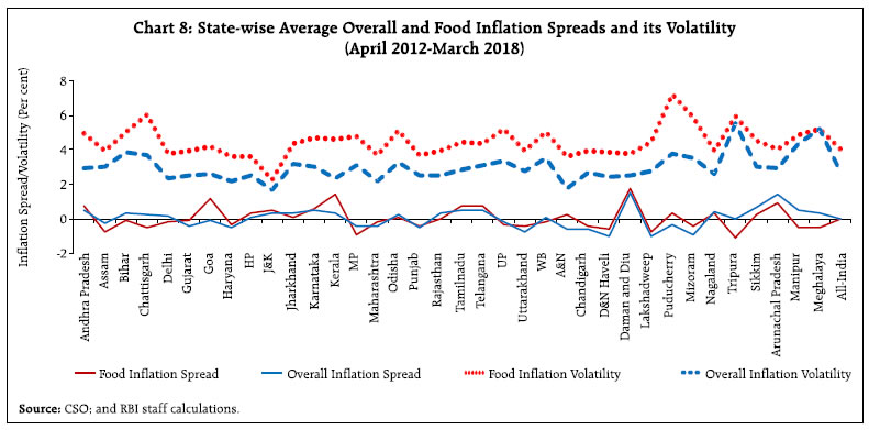
| Table 2: Results of the Panel Regression | | Explanatory Variables | Dependent Variable: Headline Inflation Spread
(20 States#; Period : 2012-13 to 2016-17) | | Coefficient | t-value | | food inflation spreadit | 0.69 | 8.80*** | | GSDP growth spreadit | -0.04 | -1.27 | | constant | 0.11 | 1.13 | | No. of observations | 100 | | F (2, 97) | 39.18*** | | R squared | 0.75 | Note: ***: represents level of significance at 1 per cent.
#: Includes Andhra Pradesh, Assam, Bihar, Gujarat, Haryana, HP, J&K, Karnataka, Kerala, Tamil Nadu, MP, Maharashtra, Odisha, Punjab, Rajasthan, UP, WB, Manipur, Meghalaya, Tripura.
Source: CSO; and RBI staff calculations. | The following equation is estimated in the regression: Headline inflation spreadit = α + β Food inflation spreadit + γGSDP growth spreadit + εit where, i stands for state, t stands for year and ε is the error term. III. The Lessons from the Literature The issue of regional inflation dynamics and convergence has attracted attention, particularly after the introduction of the Euro (Cecchetti et al, 2002; Beck et al, 2005; 2009). The primary focus has been to check the validity of the law of one price in a monetary union. Several factors have been cited - national policies designed by the government; economic, institutional and financial structures; differences in product and factor markets and the stage of economic development that the region is going through (Hendrikx and Chapple, 2002). Regions with high shares of food in consumption baskets as well as those that are heavily dependent on importing food tend to experience higher inflation than other regions. Analysis of inflation dispersion in the Euro area during 1980-2004 has found evidence supporting the convergence hypothesis – an indication of the role played by the exchange rate mechanism (ERM) (Busetti et al, 2007). A single monetary policy for the Euro area appears to have helped to stabilise inflation across member countries to a large extent. Evidence of divergence was also found, with inflation differentials across European regions observed to be large and also long-lasting (Beck et al, 2005; 2009). By contrast, price levels among cities in the US are observed to revert to mean at an exceptionally slow rate (Cecchetti et al, 2002), while socio-economic factors like income, wages, demographic structure and housing price growth explain regional price dispersions in Korea (Chang and Kim, 2017). Regional inflation and its volatility were higher in the post South-East Asian crisis period (September 1999 - July 2006) among 26 regions in Indonesia than during the pre-crisis years (Wimanda, 2006). For OECD economies, the adoption of inflation targeting contributed to a higher degree of disinflation (Ball and Sheridan, 2004). For India, significant cross-sectional dependence in prices across regions is observed for data on centre-wise CPI for Industrial Workers (CPI-IW), although relative price levels in various regions tend to mean revert (Das and Bhattacharya, 2008). The strengthening of institutions on spatial competition – product market reform (measured by state easing barriers to entrepreneurship and opening up to international trade and investment) – could lead to convergence of inflation among states (Pillai et al, 2012). IV. Testing for Convergence Given that food inflation spread drives the overall inflation spread as discussed earlier and that the food inflation spread fluctuates within a narrower range than spreads in respect of other components of inflation (Table 3), the estimated kernel density (Epanechnikov kernel, bandwidth = 0.40) of the annual average deviations of the regional inflation rates from the all-India average between April 2012 and March 2018 moves in a range of about 15 percentage points in the inflation spread experienced by different states in India (Chart 9)5. Further, the plot is more or less symmetric, implying that state-level inflation rates tend towards the national average inflation. The distribution also seems to be quite leptokurtic in nature, which could be due to the role of local price shocks in a few states in certain periods. Table 3: Inflation – Minimum, Maximum and Average Inflation Spread Volatility across States
(April 2012 to March 2018) | | Sub-groups | Minimum Inflation (in per cent) | Maximum Inflation (in per cent) | Difference between Maximum and Minimum | Inflation Spread Volatility (in percentage points) | | Food and beverages (45.9) | 5.8 | 8.7 | 2.9 | 0.67 | | Pan, tobacco and intoxicants (2.4) | 5.1 | 13.2 | 8.1 | 1.36 | | Clothing and footwear (6.5) | 5.0 | 10.2 | 5.2 | 1.03 | | Housing (10.1) | 3.4 | 9.0 | 5.6 | 1.39 | | Fuel and light (6.8) | -0.1 | 11.0 | 11.1 | 2.06 | | Miscellaneous (28.3) | 2.9 | 6.8 | 3.9 | 0.83 | | CPI-C (100) | 5.4 | 7.9 | 2.5 | 0.60 | Note: Figures in parentheses indicate the group’s weight in overall CPI-C. Inflation spread volatility is measured by the cross-sectional standard deviation of inflation divergence from all-India average.
Source: CSO; and RBI staff estimates. |
This observation seems to be validated by trends in cross-sectional variability in inflation differentials and the average inflation differentials (Chart 10). Against this backdrop, inflation convergence is tested in a random effects panel regression model (Table 4). As the Breusch-Pagan Lagrange Multiplier (LM) test suggests that an OLS regression is better suited than a random effects panel regression, the OLS results are also reported as a robustness check here (Table 5). The most widely used measures of convergence available in the literature are beta (β)-convergence and sigma (σ)-convergence (Busetti et al., 2007; Lopez and Papell, 2012; Barro and Sala-i-Martin, 1992; Mankiw et al., 1992). σ-convergence occurs when the dispersion of the levels of a given variable between different regions tends to decrease over time. In contrast, β convergence allows the identification of the speed with which shocks dissipate across regions even as the variable of interest converges towards a common benchmark (Beck and Weber, 2005)7. β convergence requires the estimation of the following equation: | Table 4: Results of the Beta Convergence Test6 | | Explanatory Variables | Dependent Variable: ∆ Inflation Spread
(36 States and UTs; Period : 2012-13 to 2017-18) | | Coefficient | Z-value | | inflation spreadit-1 | -0.77 | -6.06*** | | constant | 0.24 | 2.16** | | No. of observations | 180 | | Wald chi2(1) | 36.75*** | | R-squared | Within: 0.45; Between: 0.19; Overall: 0.41. | Note: ***, ** and * represent levels of significance at 1 per cent, 5 per cent and 10 per cent, respectively.
Source: RBI staff estimates. |
Δ inflation spreadit =α +β inflation spreadit–1+εit where, Δ is the difference operator, inflation spread measures the difference between state inflation and all-India inflation, i stands for state, t stands for year and ε is the error term. The size of β measures the speed of convergence, i.e., the speed at which regional inflation rates converge to the national average. A negative β coefficient signals the existence of convergence and the closer the absolute value of the β coefficient is to 1, the higher is the speed of convergence. The results of our analysis confirm the existence of beta convergence, i.e., convergence of regional inflation towards the national average (Tables 4 and 5). | Table 5: Results of the Beta Convergence Test | | Explanatory Variables | Dependent Variable: ∆ Inflation Spread
(36 States and UTs; Period : 2012-13 to 2017-18) | | Coefficient | t-value | | inflation spreadit-1 | -0.77 | -6.85*** | | constant | 0.24 | 1.85* | | No. of observations | 180 | | F (1, 178) | 46.90*** | | R squared | 0.4148 | Note: ***, ** and * represent levels of significance at 1 per cent, 5 per cent and 10 per cent, respectively.
Source: RBI staff estimates. | This inherent tendency of convergence of state level inflation to the national average supports the adoption of the national level CPI inflation as the nominal anchor for the conduct of monetary policy in India. V. Summary and Concluding Observations Regional inflation dynamics in India are characterised by the presence of high dispersion in inflation across states, largely reflecting regional food inflation dynamics. It is not surprising, therefore, that the food inflation spread turns out to be the primary driver of the overall inflation spread across states in our findings. The stylised facts pointing to co-movement in overall inflation across states with the all-India headline inflation are corroborated by the symmetric distribution of annual average inflation across states represented through a Kernel density function and the stationarity of the trend of cross-sectional mean inflation differentials and inflation differential variability. β convergence test confirms a reasonable pace of reversion of inflation across states towards the national average. These findings underpin the choice of the national-level CPI inflation as the nominal anchor under India’s flexible inflation targeting framework. References Ball, L. M. and N. Sheridan (2004), “Does Inflation Targeting Matter?” in ‘The Inflation-Targeting Debate’, NBER Chapters, National Bureau of Economic Research, pp. 249–282. Barro, Robert. J. and Xavier Sala-i-Martin (1992), “Convergence”, Journal of Political Economy, 100(2): 223-251. Beck, Guenter W. and Axel A. Weber (2005), “Price Stability, Inflation Convergence and Diversity in EMU: Does One Size Fit All?”, Centre for Financial Studies Working Paper No. 2005/30, November. Beck, Guenter W., Kirstin Hubrich and Massimiliano Marcellino (2009), “Regional Inflation Dynamics Within and Across Euro Area Countries and a Comparison with the United States”, Economic Policy, January, pp. 141–184. Busetti, F., F. Forni, A. Harvey and F. Venditti (2007), “Inflation Convergence and Divergence within the European Monetary Union”, International Journal of Central Banking, June. Cecchetti, Stephen G., Nelson C. Mark and Robert J. Sonora (2002), “Price Index Convergence among United States Cities”, International Economic Review, 43(4), November. Chang, Eu Joon and Young Se Kim (2017), “Regional Relative Price Disparities and Their Driving Forces”, East Asian Economic Review, September, 21(3): 201 230. Das, S. and K. Bhattacharya (2008), “Price Convergence across Regions in India”, Empirical Economics 34: 299–313. Hendrikx, M. and B. Chapple (2002), “Regional Inflation Divergence in the Context of EMU,” MEB Series (discontinued) 2002-19, Netherlands Central Bank, Monetary and Economic Policy Department. Hossain, Akhand Akhtar and Popkarn Arwatchanakarn (2016), “Inflation and Inflation Volatility in Thailand”, Applied Economics, 48(30): 2792-2806. Kim, Dong‐Hyeon and Shu‐Chin Lin (2012), “Inflation and Inflation Volatility Revisited”, International Finance, 15(3):327-345. Lopez, C. and D.H Papell (2012), “Convergence of Euro Area Inflation Rates”, Journal of International Money and Finance, Elsevier, 31(6):1440-1458. Mankiw, N.G., D. Romer and D. N. Weil (1992), “A Contribution to the Empirics of Economic Growth”, The Quarterly Journal of Economics, 107 (2): pp. 407- 437. Patra, M.D (2017), “One Year in the Life of India’s Monetary Policy Committee”, Speech delivered at the Jaipur Regional Office of RBI, Jaipur, October 27. Pillai, P.M., N. Shanta and K. Pushpangadan (2012), “Inflation in India - What do the Data Reveal about Regional Dimensions?”, Growth Development and Diversity, Oxford University Press. Weyerstrass, K., B. Aarle, M. Kappler and A. Seymen (2011), “Business Cycle Synchronisation within the Euro Area: In Search of a ‘Euro Effect’”, Open Economies Review, 22(3): 427–446. Wimanda, R.E. (2006), “Regional Inflation in Indonesia: Characteristic, Convergence, and Determinants”, Working Paper No. 13, Bank Indonesia.
|