Snehal S. Herwadkar and Bhanu Pratap* In this paper, we test whether the efficient market hypothesis works in the context of Indian banking sector. In particular, using a panel dataset of 39 publicly listed banks in India for 2009–2017, we test whether equity markets provide any lead information about stress in the banking system before quarterly data becomes available to the supervisors. We find that markets are able to price-in the banking stress concurrently but not much in advance. As the supervisory data are available with a lag, there is some merit in incorporating market-based information to track banking distress. Use of a machine learning technique to reaffirm the results is a novelty of this paper. Interestingly, our findings suggest that markets are relatively less efficient in the case of public sector banks vis-à-vis private sector banks. JEL Classification Codes: C14, C33, C51, G21, G14 Keywords: Banking sector, banking distress, equity markets, financial stability Introduction The face of banking has changed dramatically in the last couple of decades. As the range of banking activities expanded from simple borrowing and lending to more complex operations, supervisors have also tried to proactively keep pace by constantly fine-tuning their supervisory frameworks and updating the underlying models. Besides their own bank inspection data, which is the outcome of both on-site and off-site surveillance, supervisors also employ market information to assess and ensure financial stability. Since market investors require a risk premium unlike secured depositors, they incorporate all available information relating to potential risks while pricing bank stocks and forming their expectations on its likely performance in the future (Distinguin et al., 2006). For example, in the debt market, the market could penalise a bank for excessive risk-taking by demanding higher returns as compensation for higher risk. Similarly, equity prices of banks perceived to have weak financial health could decline as markets expect lower future flow of returns from investing in such scrips. If debt and equity markets are indeed efficient, market prices should accurately reflect the level of risk faced by banks and, therefore, should indicate the likelihood of emerging stress in a given bank (Krainer and Lopez, 2004b). This line of thinking is not without its share of critics. It is often argued that not all the banking equity shares are traded on a stock exchange. Even when they are, the implicit or explicit state guarantees in the form of eventual, unavoidable bailout or even in the form of lender of last resort, inhibit market prices to reflect financial position of a bank realistically. Notwithstanding these scepticisms, the academic appeal of the hypothesis has not waned. This paper attempts to evaluate whether market-based indicators help in predicting banking distress in the Indian context ahead of hard information either through quarterly accounts or through supervisory returns. While we have used stressed asset ratio as an indicator of banking distress, market-based indicators like equity returns, price-to-book value ratio and volatility, are evaluated to assess if financial markets can predict impending stress in banks. The findings suggest that in India, market variables can foretell banking distress in the same quarter, if not well in advance. As the supervisory data are available with a lag, supervisors may benefit by looking at financial market price movements while assessing banking distress. The robustness of these results was confirmed by employing the random forest algorithm from the machine learning genre. We aim to add to the literature in the following ways: first, although the usefulness of market indicators to supervisors has been extensively researched for developed countries, there is limited literature on this topic in the context of developing or emerging market economies like India. It would be a useful exercise to see how far the Indian experience is in conformity with the international evidence. Second, while research in the international arena has used non-performing assets (NPAs) as an indicator of banking stress, we have used the stressed assets ratio – which combines gross NPAs with restructured assets – as a more realistic depiction of stress in the Indian banking sector. Third, in recognition of the peculiar structure of the Indian banking sector – where public sector banks have implicit state guarantees and have also borne larger part of the recent stress – this paper extends the analysis by dividing banks on the basis of their ownership. The aim of this exercise is to examine whether markets differentiate public sector banks from their private counterparts while pricing risk. Fourth, while we present a panel fixed effect model using several alternative specifications, the analysis is complemented with a random forest model which serves as an effective cross-validation without any a priori specification. The rest of the article is organised as follows: Section II presents the review of the literature, while Section III elaborates on the data, the empirical analysis and the results. Section IV concludes the paper and evaluates policy implications. Section II Review of Literature Literature suggests a wide range of market-based predictors, including movements in insured and uninsured deposits, debt instruments and bank equity returns, as potential candidates to supplement the supervisory efforts. Banking stress is reflected in the financial markets through several channels, which can be classified into direct and indirect impact, as well as into quantity and price-based impact. In direct quantity impact, the bank perceived as risk-prone experiences gradual or sudden withdrawal of deposits. In contrast, in the indirect quantity impact, bank creditors restructure their holdings, thereby signalling their concerns to the bank. Another layer could also be involved in this channel, whereby supervisors or private agents make it mandatory for the bank to reduce its risks. Thus, both the direct as well as indirect channels imply movement of funds from ‘risky’ to ‘safer’ banks, converting uninsured funds to insured funds, obtaining collateral, and cancelling existing banking relationships (Bennett et al., 2015). The direct price mechanism manifests itself when a bank is forced to pay higher risk premiums on at-risk liabilities (e.g., uninsured deposits) or suffer other risk-based cost increases (e.g., higher credit default swap spreads) when its risk increases. Finally, indirect price discipline occurs when the equity prices of a risk-prone bank decline more than the market thereby sending signals to investors as well as to the bank management. These adverse wealth effects may be expected to prompt the majority stakeholders or bank supervisors to force the bank to take corrective action. This paper is focussed on India where, partly due to an implicit government guarantee, banking activity is largely perceived to be low risk, and major quantity impact, such as a bank run, has been largely absent. Taking a cue from the literature, which suggests that at low levels of risk the price mechanism dominates the quantity mechanism in disciplining the banks, we focus on price mechanism, particularly in equity markets, and prepare the ground through a detailed survey of the literature on this aspect. Moreover, by focusing on equity market-based predictors for banking stress, we derive motivation from Caldwell (2007), who compared three market instruments, viz., equity, subordinated debentures and uninsured deposits for their effectiveness in disciplining banks’ risk choice and found that equity weakly dominates the other two instruments. Elmer and Fissel (2001) and Krainer and Lopez (2004a, 2004b) found evidence of equity markets providing information that can help in predicting bank distress, thus advocating use of this information in the supervisory review process. Earlier, Flannery (1998), González-Hermosillo (1999) and Jagtiani and Lemieux (2001) also emphasised the importance of combining market-based indicators with macroeconomic data for prior information on banking stress. Curry et al. (2003) documented evidence that stock prices incorporate banking distress as much as two years ahead of the supervisory rating downgrade. In addition, their findings suggested that adding market variables to standard models with bank financial data improved the predictive power of these models, albeit marginally. Based on empirical evidence for banks in the Eurozone, Distinguin et al., (2006) and Gropp et al., (2006) suggested creation of early-warning systems based on market information. Borio and Lowe (2002), who examined three sets of possible predictors of a banking crisis – credit gap, real equity gap and real exchange rate gap, each measured in terms of deviation from Hodrick-Prescott filtered trend – found that while the credit and exchange rate gaps tend to rise one year before the crisis and peak during the crisis year, the equity prices tend to fall in the year immediately preceding the crisis. Their findings also suggest that a composite indicator consisting of credit and asset prices is a superior predictor of banking crises compared with other alternatives because of its high predictive power and lower noise-to-signal ratio, especially at longer horizons. Taking a slightly different stance, some researchers found that bank-specific characteristics such as reliance on short-term funding, more leverage and hunger for quick growth make some banks more sensitive to crisis than others. Analysing a sample of 347 banking firms in the US between 1998 and 2006, Fahlenbrach et al., (2012) showed that a bank’s stock return performance during the 1998 crisis helped in predicting both its stock return performance and probability of failure during the recent global financial crisis. The authors concluded that persistence in a bank’s risk culture and business model make their performance sensitive to crisis. Along with studies that recommend the use of market variables to aid supervisory process, contradictory line of thinking also exists in the literature, making the debate inconclusive. For example, Berger et al. (2000) examined the relationship between supervisory information and several market indicators such as rating changes, and abnormal stock returns. Their results suggested that the supervisory assessments and bond ratings complement each other, partly because both agencies are concerned with bankruptcy risk. In contrast, supervisory assessments and equity indicators are not strongly related reflecting the fact that the latter concentrate more on wealth creation which is essentially a non-default risk feature. In the Indian context, Mishra and Sreeramulu (2017) constructed three separate indices to gauge banking stress, viz., index of speculative pressures, index of macroeconomic vulnerability and index of banking sector vulnerability, using several macro-financial indicators. The present paper takes this strand of literature further by empirically testing the predictive power of equity market variables in predicting banking stress. Section III Data, Methodology and Results We estimate a panel fixed effect model using quarterly accounting and supervisory data of 39 publicly listed, scheduled commercial banks1 (SCBs). The equity market performance of each bank, including excess return on bank scrip compared to the banking sector as a whole, market capitalisation, price-to-book value ratio and 90-day realised volatility of each bank stock, represent the equity market variables. The NPA ratios are widely used in the literature as proxies for banking distress (e.g., Beck et al., 2015). We have, however, used the stressed assets ratio as a proxy, which takes into account not only the NPAs but also the restructured assets, in recognition of the fact that before the asset quality review (AQR) in 2015, the NPA ratio of Indian banks did not portray a realistic picture of the defaults. Lastly, we also use a machine learning method, namely random forest algorithm to reinforce the findings of the panel fixed effects model (Appendix A). Like any other machine learning method, the random forest algorithm makes almost no a priori assumptions on the underlying relationship between the target and predictor variables. Additionally, the algorithm is designed to use bootstrapped method to learn from the data to make predictions. Such features of the random forest approach make it robust even in the presence of a large number of highly collinear variables. In particular, we use the variable importance, computed using the random forest algorithm, to assess the predictive ability of financial market variables. However, unlike econometric techniques, this method does not provide the level of significance or direction of causality for such estimates. Considering factors like availability of data, the time period for the analysis was set from 2009:Q1 to 2017:Q4 (Appendix B and C). Incidentally, this period is crucial for the Indian banking sector as the health of the banking system was considered robust at the beginning of this period but observed sharp deterioration midway through. Thus, this period provides the right window to test the hypothesis whether market indicators are better predictors of banking distress. Bank-wise Stressed Assets and Market Information: Fixed Effects Panel Model A fixed effect model, in line with Beck et al., (2015), is estimated with stressed assets ratio (SAR) as the dependent variable. The basic objective was to test whether financial market variables are able to anticipate banking stress over and above the supervisory data, and if so, then how much in advance. In order to test whether markets anticipate stress in advance, we also introduce up to two lags in the financial market explanatory variables. Thus, ceteris paribus, if the coefficients of the one (two) quarter lagged financial market variables turn out to be significant, we deduce that the financial markets anticipate stress one (two) quarter ahead and that the financial markets are strongly efficient in anticipating the stress in banks. We estimate a baseline model for bank distress that includes one quarter lagged supervisory variables controlling for size (assets), profitability (return on equity i.e., RoE), and capital (capital to risk-weighted assets i.e., CRAR):  The motivation behind the usage of the one-period lagged independent variables is that supervisory returns data for the current quarter are available with a time lag of close to one to three months after the end of a given quarter. Therefore, an assessment of bank-level stress at any given point of time is possible on the basis of one quarter old information, which might be an outdated information from the point of view of financial stability. In addition to cross-section fixed effects to control bank-level heterogeneity, we also allow for time fixed effects2 in the model to control for macroeconomic and regulatory policies that uniformly impact all banks. Finally, to control for cross-sectional dependence3 arising from several factors like sample selection, unobserved shocks and policies, we estimate the model with Driscoll-Kraay robust standard errors (Driscoll and Kraay, 1998) using the algorithmic routine provided by Hoechle (2007). Such standard errors are also robust to heteroscedastic and autocorrelated disturbances. Building on this baseline specification, we then introduce one by one contemporaneous, one- and two-period lagged values of equity market variables in the model to ascertain the predictive power of equity markets. Equation (2) represents weak efficiency of the financial markets, where they anticipate the stress in the same period such that j = 0. In particular, we test a variety of signals provided by the equity markets, viz., stock returns adjusted to NSE Nifty Bank Index (Ret. Niftybank); price-to-book value ratio (PB Ratio) of a bank stock which reflects the value that market participants attach to the bank’s equity relative to its book value; and observed volatility (Volatility) in the bank’s stock4. As mentioned earlier, if financial markets are indeed forward-looking, lagged values of market variables should return statistical significance (for j = 1 or 2). The estimation results for the full sample are provided in Appendix Table D5. The results suggest that financial markets pick up signals of banking distress in the same quarter but not much in advance, and thus are at best, weakly efficient in predicting the same. The results suggest a contemporaneous statistical relationship between market variables and stressed assets ratio; with the coefficients of the lagged values of equity market variables lacking statistical significance except in the case of one-period lagged price-to-book value ratio and two-period lagged volatility. Compared to the baseline, only a marginal improvement in the overall R2 of the models after incorporating market information, also suggests weak statistical power of market information5. Given the heterogeneous nature of the Indian banking system, we also examine whether the ownership pattern of banks makes a difference to equity markets reaction. Thus, we split our sample into public sector bank and private sector banks subsamples and estimate the same model as in equation (2) for both the subsamples. The estimation results are provided in Appendix Tables D6 and D7. For the public sector banks, asset base and CRAR showed inverse association with SAR as expected. However, the coefficient of return on equity (RoE) was not statistically significant. Regarding the predictive power of equity markets, none of the equity market variables were found to have a statistically significant relationship with SAR, even at 10 per cent level of significance. The only exception to this was the two quarter lagged observed volatility in the bank stock price, which might signal trading activity on a bank stock on account of policy announcements such as recapitalisation. On the other hand, results for the private sector banks depict a more sanguine story. Specifically, the price-to-book value ratio was found to contain more meaningful information to predict bank-level distress. Price-to-book value ratio is simply the market price per share divided by the book value per share. Thus, it can be argued that price-to-book value ratio contains information from the balance sheet of a bank as well as the market’s expectations in the form of its share price. In the case of private sector banks, therefore, it seems that equity markets do make their own assessment of impending stress on the balance sheet of a bank. Model 11 in Table D7 incorporates stock returns, price-to-book-value and volatility albeit leading to only a slight improvement in the R2 with respect to the baseline model. The results of the public and private sector banks indicate that the markets differentiate their anticipation of stress based on ownership pattern. Acquisition, verification and pricing of information is costly. For public sector banks, which have implicit state guarantees, these costs seem to outweigh the benefits. In particular, if the investors are confident that the stress on a public sector bank – however grave it may be – would be relieved by the government through various means such as recapitalisation, then the market has little incentive to price-in the stress. Stressed assets affect bank’s balance sheet because they involve higher provisioning and reduce the lendable resources available with banks. However, if the government stands ready to recapitalise the banks then the stress on their balance sheet is relieved automatically. Factoring in these considerations, markets may be providing meaningful information about the impending stress in case of private sector banks but not in the case of public sector banks. Machine Learning-based Assessment The random forest (RF) algorithm6, a popular technique from the machine learning paradigm, is a useful alternative method that can be used to confirm the findings of the econometric model. The RF algorithm allows the computation of variable importance to assess the relative importance of a variable in a regression (when the dependent/target variable is continuous) or classification (when the dependent/target variable is binary) problem. The basic building block of the RF algorithm is a decision tree, which can be depicted in the form of a flowchart-like graph to illustrate all possible outcomes of a decision or a series of decisions. A decision tree splits the input parameter space into non-overlapping subsamples, such that the predicted value of the target variable in each subsample is a constant value contingent on minimisation of overall residual sum of squares (RSS). Decision trees, however, are prone to an overfitting problem. In contrast, as a non-parametric, supervised machine learning model, the RF algorithm avoids this problem by way of bagging or bootstrapped aggregation. First, it grows a collection or ensemble of decision trees. Second, it uses a random, bootstrapped sample of input data as well as a random subset of input variables to grow each tree. This simple modification of using a random subset of input variable for growing each tree, de-correlates individual trees to reduce the variance in the overall prediction. Third, for each tree, it calculates a prediction error using out-of-bag (OOB) data, i.e., data left out from the initial sample for that tree. Lastly, with the aim to minimise prediction error, it averages out the predictions from all individual trees to arrive at a final prediction. Thus, random forests can efficiently deal with very large numbers of correlated explanatory variables, and the predicted model is highly non-linear. As mentioned earlier, while training the model, the algorithm calculates the prediction error on OOB data that was not used during its training. This step allows the computation of variable importance that can be used to select the most important predictors amongst a large batch of potential predictor variables. The algorithm can be trained to solve the following regression task to predict bank-level distress: 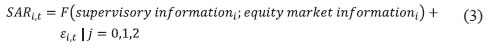 We note that while implementing the panel fixed effect model, only a limited number of dependent variables7 – whether supervisory or market-based – were used in order to achieve a best fit while avoiding the multicollinearity problem. Since the RF algorithm can efficiently deal with correlated variables, the entire set of independent variables (including those on bank size, capital, profitability, deposit ratios, etc.) available at our disposal were utilised as a set of potential predictors. Like the fixed-effect regression approach, we control for bank and time fixed effects by introducing bank-specific dummies and some macroeconomic variables in the set of input variables, respectively. Full sample data is used for training the model since our primary interest is in assessing the importance of a given variable as a predictor of the target variable. The rankings of important predictor variables, in terms of increase in mean squared error (MSE), are provided in Chart 1. The higher the increase in MSE of any given predictor variable, higher the importance of that variable. Clearly, bank regulatory capital and profitability are the strongest predictors of banking distress. Indicators such as Tier-2 capital ratio, total CRAR, return on assets (RoA), net interest margin (NIM) occupy top ranking in the variable importance measure. Similarly, short-term liquidity, proxied by savings deposits ratio and liquid assets ratio, also emerge as important predictors. In line with the findings of the fixed effect panel model, the random forest approach also ranked market variables as the least important predictors of banking distress. Moreover, in a relative sense, most of the market indicators show very low percentage increase in MSE which underlines the low predictive power contained in equity market information. Lagged values of market variables do not even appear in the top predictors. To further analyse the impact of market variables on predicting bank distress, we retrain the model without including market variables in the training data set. We find no meaningful impact of the exclusion of financial market information on the overall predictive accuracy of the model. The findings8 are also robust to changes in the hyper-parameters of the model – number of trees grown, number of nodes on each tree and number of variables used in each iteration. 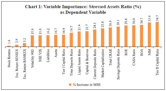 Section V Conclusion The primary aim of this analysis is to determine the incremental predictive value of market information over and above that provided by the supervisory information. The paper finds evidence that the market variables incorporate information about banks’ stress in the same quarter, though not much in advance and thus markets are weakly efficient. Considering, however, that the supervisory data are available with a lag, the paper suggests that there is some merit in using market variables to identify stress in the banking sector. The random forest model – which ranks variables in terms of their importance in predicting stress – also confirms the findings of the fixed effect panel model by allotting lower ranks to market variables as compared with the supervisory variables. More significantly, our results suggest that the markets differentiate between banks on the basis of their ownership while incorporating information about stress in stock prices. This may be because public sector banks are perceived to have an implicit sovereign guarantee against failure, thereby reducing incentives to monitor them, which may be weakening the market discipline channel.
References Beck, R., Jakubik, P., & Piloiu, A. (2015). Key determinants of non-performing loans: New evidence from a global sample. Open Economies Review, 26(3), 525–550. Bennett, R. L., Hwa, V., & Kwast, M. L. (2015). Market discipline by bank creditors during the 2008–2010 crisis. Journal of Financial Stability, 20, 51–69. Berger, A., Davies, S., & Flannery, M. (2000). Comparing market and supervisory assessments of bank performance: Who knows what when? Journal of Money, Credit and Banking, 32(3), 641–667. doi:10.2307/2601200 Borio, C., & Lowe, P. (2002). Assessing the risk of banking crises. BIS Quarterly Review, 7(1), 43–54. Breiman, L. (2001). Random forests. Machine learning, 45(1), 5–32. Caldwell, G. (2007). Best instruments for market discipline in banking, Staff Working Paper No. 2007-9. Bank of Canada. https://www.bankofcanada.ca/2007/02/working-paper-2007-9/ Curry, T. J., Elmer, P. J., & Fissel, G. S. (2003). Using market information to help identify distressed institutions: A regulatory perspective. FDIC Banking Review, 15(3), 1–16. Distinguin, I., Rous, P., & Tarazi, A. (2006). Market discipline and the use of stock market data to predict bank financial distress. Journal of Financial Services Research, 30(2), 151–176. Driscoll, J. C., & Kraay, A. C. (1998). Consistent covariance matrix estimation with spatially dependent panel data. Review of Economics and Statistics, 80(4), 549–560. Elmer, P. J., & Fissel, G. (2001). Forecasting bank failure from momentum patterns in stock returns. Unpublished paper, Federal Deposit Insurance Corporation, US. Fahlenbrach, R., Prilmeier, R., & Stulz, R. M. (2012). This time is the same: Using bank performance in 1998 to explain bank performance during the recent financial crisis. The Journal of Finance, 67(6), 2139–2185. Fisher, A., Rudin, C., & Dominici, F. (2019). All models are wrong, but many are useful: Learning a variable’s importance by studying an entire class of prediction models simultaneously. Journal of Machine Learning Research, 20(177), 1–81. Flannery, M. J. (1998). Using market information in prudential bank supervision: A review of the US empirical evidence. Journal of Money, Credit and Banking, 273–305. González-Hermosillo, B. (1999). Developing indicators to provide early warnings of banking crises. Finance and Development, 36, 36–39. Gropp, R., Vesala, J., & Vulpes, G. (2006). Equity and bond market signals as leading indicators of bank fragility. Journal of Money, Credit and Banking, 38(2), 399–428. Hoechle, D. (2007). Robust standard errors for panel regressions with cross-sectional dependence. The Stata Journal, 7(3), 281–312. Jagtiani, J., & Lemieux, C. (2001). Market discipline prior to bank failure. Journal of Economics and Business, 53(2–3), 313–324. James, G., Witten, D., Hastie, T., & Tibshirani, R. (2013). An introduction to statistical learning (Vol. 112, pp. 3-7). New York: Springer. Krainer, J., & Lopez, J. A. (2004a). Using securities market information for bank supervisory monitoring. FRBSF Working Paper 2004-05. Federal Reserve Bank of San Francisco. https://www.frbsf.org/economic-research/files/wp04-05bk.pdf Krainer, J., & Lopez, J. A. (2004b). Incorporating equity market information into supervisory monitoring models. Journal of Money, Credit and Banking, 36(6), 1043–1067. Liaw, A., & Wiener, M. (2002). Classification and regression by random Forest. R News, 2(3), 18–22. Mishra, Rabi N. and Sreeramulu, M. (2017). Forewarned is forearmed: Configuring an early warning mechanism for macro-financial space in India, September 21. https://ssrn.com/abstract=3040463 or http://dx.doi.org/10.2139/ssrn.3040463 Torres-Reyna, O. (2007). Panel data analysis fixed and random effects using Stata (v. 4.2). Data & Statistical Services, Princeton University. https://www.princeton.edu/~otorres/Panel101.pdf
APPENDIX A Random Forest Algorithm: A Summary Decision Tree In supervised machine learning, tree-based methods are popular for solving both regression (when target variable is continuous) and classification (when target variable is binary) problems. Such methods generate prediction through rules derived from recursive binary partitioning of the covariate space. In other words, a regression tree method splits the predictor space into a number of smaller regions, wherein the mean or mode of all observations falling in that region is used as a prediction for any given observation in the same region. A typical decision tree model to predict a target variable, say Y, given two predictors, say X1, X2, can be represented as shown in Figure A.1. 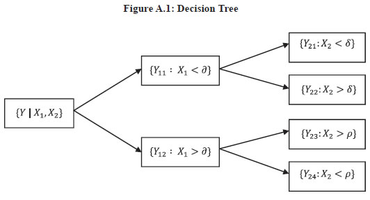 More formally, the covariate space i.e., the set of possible values of X1, X2 ... ... XN is divided into J distinct and non-overlapping regions, R1, R2 ... ... RJ. For each observation in region RJ, the prediction is simply ŶR j i.e., the mean of all observations falling within the same region. Given predictor XN and a cut-off point SNi for each such predictor, the optimal division of the covariate space is achieved by recursively minimising the following residual sum of squares (RSS): Random Forest Algorithm Decision trees discussed above suffer from the issue of high variance or overfitting. To overcome this issue, several strategies have been highlighted in the literature. Bootstrapped aggregation or bagging is one such procedure, which when applied to decision trees is popularly known as the random forest algorithm. Proposed by Breiman (2001), the algorithm includes the construction of T decision trees using distinct bootstrapped subsamples of input data. While constructing each tree, the algorithm uses n < N predictor variables chosen at random. This small tweak over conventional bagging results in a decorrelation of regression trees. After all the trees are constructed, the algorithm generates a final prediction by averaging the prediction of all T regression trees. Formally, each tree in a random forest is built using the following steps where T represents the entire forest and t represents a single tree. For t = 1 to T: Out-of-bag Error Estimation and Variable Importance Recall that the random forest algorithm uses a bootstrapped input sample data for training each regression tree. In Breiman’s proposed algorithm, each bagged regression tree uses two-thirds of the input data for construction. The input data that is left out from such a sample is termed out-of-bag (OOB) data. A straightforward way to estimate the test error of a random forest model is to use the OOB data. A mean prediction for each ith observation can be obtained by averaging the prediction of each tree in which the observation was OOB. This way an OOB mean squared error (MSE) can be computed for the random forest model: which is considered a valid estimate of the test error for the model since the response for each observation is predicted using the trees that were not fit using the same observation. The random forest model, by obtaining an MSEooB, allows the computation of variable importance which can be used to select most important predictors amongst a large batch of potential predictor variables. Variable importance is said to describe the dependence of a model’s prediction accuracy on the information contained in each covariate used by the model (Fisher et al., 2019). The importance of a variable say XN , is estimated by computing the increase in mean prediction error when the OOB data, with the nth input variable randomly permuted, is again passed down the tree(s) to make predictions. Intuitively, the random shuffling of the nth variable would mean that the shuffled variable has no predictive power. The mean increase in prediction error is computed for all variables – the larger the increase in prediction error for any given variable, higher is the predictive power of that variable. The variable importance (VIN ) for each variable is computed as follows:
Appendix B Data Description and Sources | Variable | Description | Frequency | Source | | Stressed Assets Ratio (%) | (Restructured Standard Advances + Gross Non-Performing Advances) / Total Gross Advances | Quarterly | Supervisory Returns, RBI | | Assets (INR billions) | Total Assets of the Bank | Quarterly | Supervisory Returns, RBI | | Current Deposits Ratio (%) | Total Current Deposits / Total Assets | Quarterly | Supervisory Returns, RBI | | Time Deposits Ratio (%) | Total Term Deposits / Total Assets | Quarterly | Supervisory Returns, RBI | | Savings Deposits Ratio (%) | Total Savings Deposits / Total Assets | Quarterly | Supervisory Returns, RBI | | CASA Ratio (%) | (Total Current Deposits + Total Savings Deposits) / Total Assets | Quarterly | Supervisory Returns, RBI | | Capital & Reserves | Total Capital & Reserves / Total Assets | Quarterly | Supervisory Returns, RBI | | Liquid Assets Ratio (%) | Total Liquid Assets / Total Assets | Quarterly | Supervisory Returns, RBI | | Total CRAR (%) | Total Regulatory Capital / Risk-Weighted Total Assets of the Bank | Quarterly | Supervisory Returns, RBI | | Tier 1-Capital Ratio (%) | Total Tier 1 Regulatory Capital / Risk- Weighted Total Assets of the Bank | Quarterly | Supervisory Returns, RBI | | Tier 2-Capital Ratio (%) | Total Tier 2 Regulatory Capital / Risk- Weighted Total Assets of the Bank | Quarterly | Supervisory Returns, RBI | | Return on Assets (%) | Total Net Profits / Average Total Assets | Quarterly | Supervisory Returns, RBI | | Return on Equity (%) | Total Net Profits / Average Total Shareholders' Equity for the Bank | Quarterly | Supervisory Returns, RBI | | Net Interest Margin (%) | Net Interest Income / Average Total Assets | Quarterly | Supervisory Returns, RBI | | VIX | NSE VIX Index | Quarterly | Bloomberg | | Excess Return over NSE Bank (%) | 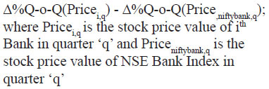 | Quarterly | Bloomberg; Authors’ calculation | | Excess Return over NSE Bank (%) | 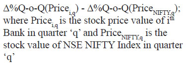 | Quarterly | Bloomberg; Authors’ calculation | | Price-to-Book Ratio | Market price per share / Book value per share; where book value per share is equal to (total assets – total liabilities) / number of shares outstanding | Quarterly | Bloomberg | | Market Capitalisation | (Current market price per share) x (Total number of shares outstanding); | Quarterly | Bloomberg | | 90-d Price Volatility | Standard deviation of daily logarithmic price changes for the 90 most recent trading days closing price | Quarterly | Bloomberg |
Appendix C Summary Statistics | Table C1: All Scheduled Commercial Banks | | Variable | Obs. | Mean | Std. Dev. | Min. | Max. | | Stressed Assets Ratio (%) | 1,404 | 8.65 | 5.85 | 0.00 | 29.49 | | Assets (INR billions) | 1,404 | 2.068 | 2.771 | 0.00 | 2.883 | | Total CRAR (%) | 1,404 | 12.86 | 2.36 | 0.00 | 20.61 | | Return on Equity (%) | 1,404 | 9.59 | 10.51 | -46.97 | 41.48 | | Return over NSE Bank (%) | 1,404 | -0.97 | 6.67 | -25.92 | 41.17 | | Price-to-Book Ratio | 1,404 | 1.14 | 1.14 | 0.00 | 7.17 | | Market Capitalisation (INR billions) | 1,404 | 2.404 | 5.067 | 0.00 | 4.845 | | 90-d Stock Volatility | 1,404 | 36.37 | 11.62 | 0.00 | 88.40 |
| Table C2: Public Sector Banks | | Variable | Obs. | Mean | Std. Dev. | Min. | Max. | | Stressed Assets Ratio (%) | 864 | 11.00 | 5.83 | 0.00 | 29.49 | | Assets (INR billions) | 864 | 2.565 | 3.155 | 0.00 | 2.883 | | Total CRAR (%) | 864 | 11.91 | 1.78 | 0.00 | 18.18 | | Return on Equity (%) | 864 | 7.76 | 11.33 | -46.97 | 41.48 | | Return over NSE Bank (%) | 864 | -1.74 | 6.76 | -25.92 | 37.44 | | Price-to-Book Ratio | 864 | 0.63 | 0.42 | 0.00 | 2.85 | | Market Capitalisation (INR billions) | 864 | 1.515 | 3.361 | 0.00 | 2.675 | | 90-d Stock Volatility | 864 | 37.33 | 11.32 | 0.00 | 88.40 |
| Table C3: Private Sector Banks | | Variable | Obs. | Mean | Std. Dev. | Min. | Max. | | Stressed Assets Ratio (%) | 540 | 4.89 | 3.43 | 0.00 | 21.54 | | Assets (INR billions) | 540 | 1.273 | 1.739 | 0.00 | 9.246 | | Total CRAR (%) | 540 | 14.37 | 2.37 | 7.44 | 20.61 | | Return on Equity (%) | 540 | 12.53 | 8.23 | -33.96 | 29.68 | | Return over NSE Bank (%) | 540 | 0.27 | 6.34 | -25.15 | 41.17 | | Price-to-Book Ratio | 540 | 1.95 | 1.42 | 0.00 | 7.17 | | Market Capitalisation (INR billions) | 540 | 3.826 | 6.743 | 0.00 | 4.850 | | 90-d Stock Volatility | 540 | 34.82 | 11.93 | 12.65 | 86.17 |
Appendix D Diagnostic Tests and Estimation Results Table D1: Joint Wald Test of Significance for Inclusion of Time-Fixed Effects
(Null: αt = 0 for all t) | | F (34, 38) | 39.20 | | Prob. > F | 0.000 |
Table D2: Modified Wald Test for Group-wise Heteroscedasticity in Fixed Effect
Regression Model (Null: sigma(i)^2 = sigma^2 for all i) | | chi2 (39) | 3294.78 | | Prob. > chi2 | 0.000 |
Table D3: Wooldridge Test for Autocorrelation in Panel Data
(Null: No First Order Autocorrelation) | | F (1, 38) | 5.721 | | Prob. > F | 0.0218 |
Table D4: Pesaran's Test of Cross-sectional Independence
(Null: No Cross-sectional Dependence) | | test-stat | -2.687 | | Prob. | 0.0072 |
| Table D5: Estimation Results for Fixed Effect Panel Model (Sample – Full Sample) | | Independent Variable ↓ | (1) | (2) | (3) | (4) | (5) | (6) | (7) | (8) | (9) | (10) | (11) | | Dependent Variable → | SAR | SAR | SAR | SAR | SAR | SAR | SAR | SAR | SAR | SAR | SAR | | Assets (-1) (in Logs) | -0.087***
(0.0055) | -0.089***
(0.0053) | -0.088***
(0.0055) | -0.090***
(0.0051) | -0.084***
(0.0049) | -0.083***
(0.0055) | -0.085***
(0.0059) | -0.083***
(0.0065) | -0.083***
(0.0066) | -0.081***
(0.0050) | -0.067***
(0.0061) | | RoE(-1) | -0.19***
(0.028) | -0.18***
(0.028) | -0.18***
(0.028) | -0.18***
(0.030) | -0.18***
(0.029) | -0.18***
(0.029) | -0.18***
(0.031) | -0.19***
(0.027) | -0.18***
(0.027) | -0.18***
(0.029) | -0.16***
(0.028) | | CRAR (-1) | -0.38***
(0.078) | -0.38***
(0.080) | -0.38***
(0.079) | -0.38***
(0.081) | -0.37***
(0.075) | -0.38***
(0.076) | -0.38***
(0.079) | -0.37***
(0.079) | -0.36***
(0.081) | -0.37***
(0.084) | -0.32***
(0.086) | | Adj.Ret | | -0.041*
(0.018) | | | | | | | | | -0.043*
(0.020) | | Adj.Ret(-1) | | | -0.020
(0.014) | | | | | | | | -0.043*
(0.019) | | Adj.Ret(-2) | | | | -0.034
(0.020) | | | | | | | | | PB Ratio | | | | | -0.0087*
(0.0034) | | | | | | -0.0064**
(0.0018) | | PB Ratio(-1) | | | | | | -0.0066*
(0.0029) | | | | | | | PB Ratio(-2) | | | | | | | -0.0054
(0.0036) | | | | | | Vol.90d | | | | | | | | 0.00030
(0.00016) | | | | | Vol.90d(-1) | | | | | | | | | 0.00033
(0.00018) | | | | Vol.90d(-2) | | | | | | | | | | 0.00050***
(0.00011) | 0.00034**
(0.000099) |
| Constant | 1.23***
(0.069) | 1.25***
(0.066) | 1.24***
(0.069) | 0
(.) | 1.20***
(0.061) | 1.19***
(0.068) | 0
(.) | 1.18***
(0.087) | 1.17***
(0.088) | 0
(.) | 0
(.) | | Bank FE | Y | Y | Y | Y | Y | Y | Y | Y | Y | Y | Y | | Time FE | Y | Y | Y | Y | Y | Y | Y | Y | Y | Y | Y | | N | 1358 | 1358 | 1358 | 1319 | 1358 | 1358 | 1319 | 1358 | 1358 | 1319 | 1303 | | R2(within) | 0.6508 | 0.6538 | 0.6516 | 0.6547 | 0.6550 | 0.6534 | 0.6542 | 0.6537 | 0.6544 | 0.6607 | 0.6589 | | Note: Standard errors in parentheses; * p < 0.05, ** p < 0.01, *** p < 0.001. |
| Table D6: Estimation Results for Fixed Effect Panel Model (Sample – Public Sector Banks) | | Independent Variable ↓ | (1) | (2) | (3) | (4) | (5) | (6) | (7) | (8) | (9) | (10) | (11) | | Dependent Variable → | SAR | SAR | SAR | SAR | SAR | SAR | SAR | SAR | SAR | SAR | SAR | | Assets (-1) (in Logs) | -0.13***
(0.021) | -0.13***
(0.021) | -0.13***
(0.021) | -0.14***
(0.016) | -0.13***
(0.023) | -0.13***
(0.022) | -0.14***
(0.018) | -0.13***
(0.022) | -0.13***
(0.022) | -0.14***
(0.017) | -0.14***
(0.018) | | RoE (-1) | -0.067
(0.037) | -0.061
(0.038) | -0.065
(0.037) | -0.069
(0.038) | -0.067
(0.036) | -0.067
(0.037) | -0.072
(0.038) | -0.069
(0.037) | -0.067
(0.036) | -0.075
(0.037) | -0.065
(0.039) | | CRAR (-1) | -0.84***
(0.21) | -0.83***
(0.20) | -0.84***
(0.21) | -0.85***
(0.20) | -0.84***
(0.22) | -0.84***
(0.23) | -0.85***
(0.23) | -0.84***
(0.22) | -0.84***
(0.22) | -0.84***
(0.22) | -0.82***
(0.21) | | Adj.Ret. | | -0.051
(0.028) | | | | | | | | | -0.052
(0.029) | | Adj.Ret.(-1) | | | -0.024
(0.016) | | | | | | | | -0.040
(0.023) | | Adj.Ret.(-2) | | | | -0.045
(0.027) | | | | | | | | | PB Ratio | | | | | 0.00023
(0.0064) | | | | | | -0.0017
(0.0041) | | PB Ratio(-1) | | | | | | 0.0023
(0.0058) | | | | | | | PB Ratio(-2) | | | | | | | 0.00089
(0.0068) | | | | | | Vol.90d | | | | | | | | 0.00018
(0.00018) | | | | | Vol.90d(-1) | | | | | | | | | 0.00018
(0.00022) | | | | Vol.90d(-2) | | | | | | | | | | 0.00041***
(0.00011) | 0.00030**
(0.000098) |
| Constant | 0
(.) | 0
(.) | 0
(.) | 2.01***
(0.22) | 0
(.) | 0
(.) | 2.00***
(0.25) | 0
(.) | 0
(.) | 1.95***
(0.24) | 0
(.) | | Bank FE | Y | Y | Y | Y | Y | Y | Y | Y | Y | Y | Y | | Time FE | Y | Y | Y | Y | Y | Y | Y | Y | Y | Y | Y | | N | 834 | 834 | 834 | 810 | 834 | 834 | 810 | 834 | 834 | 810 | 798 | | R2(within) | 0.7408 | 0.7436 | 0.7415 | 0.7436 | 0.7408 | 0.7410 | 0.7412 | 0.7416 | 0.7416 | 0.7455 | 0.7374 | | Note: Standard errors in parentheses; * p < 0.05, ** p < 0.01, *** p < 0.001. |
| Table D7: Estimation Results for Fixed Effect Panel Model (Sample – Private Sector Banks) | | Independent Variable ↓ | (1) | (2) | (3) | (4) | (5) | (6) | (7) | (8) | (9) | (10) | (11) | | Dependent Variable → | SAR | SAR | SAR | SAR | SAR | SAR | SAR | SAR | SAR | SAR | SAR | | Asset (-1) (In Logs) | -0.036***
(0.0061) | -0.037***
(0.0059) | -0.036***
(0.0062) | -0.038***
(0.0061) | -0.034***
(0.0056) | -0.033***
(0.0057) | -0.034***
(0.0059) | -0.036***
(0.0067) | -0.035***
(0.0066) | -0.037***
(0.0059) | -0.028**
(0.0091) | | RoE (-1) | -0.23***
(0.026) | -0.23***
(0.026) | -0.23***
(0.026) | -0.22***
(0.027) | -0.21***
(0.028) | -0.22***
(0.028) | -0.22***
(0.029) | -0.23***
(0.026) | -0.22***
(0.026) | -0.22***
(0.028) | -0.20***
(0.029) | | CRAR (-1) | -0.21**
(0.070) | -0.21**
(0.069) | -0.21**
(0.070) | -0.22**
(0.075) | -0.20**
(0.073) | -0.22**
(0.076) | -0.22*
(0.082) | -0.21**
(0.072) | -0.20**
(0.067) | -0.22**
(0.077) | -0.20*
(0.097) | | Adj.Ret. | | -0.031**
(0.0090) | | | | | | | | | -0.030**
(0.0096) | | Adj.Ret. (-1) | | | -0.0042
(0.014) | | | | | | | | -0.027*
(0.012) | | Adj.Ret. (-2) | | | | -0.015
(0.013) | | | | | | | | | PB Ratio | | | | | -0.0071**
(0.0025) | | | | | | -0.0065***
(0.0017) | | PB Ratio(-1) | | | | | | -0.0057*
(0.0024) | | | | | | | PB Ratio(-2) | | | | | | | -0.0053*
(0.0024) | | | | | | Vol.90d | | | | | | | | -0.000016 (0.00013) | | | | | Vol.90d (-1) | | | | | | | | | 0.00014
(0.00010) | | | | Vol.90d (-2) | | | | | | | | | | 0.00006
(0.0001) | 0.00004
(0.0001) |
| Constant | 0.53***
(0.072) | 0.54***
(0.069) | 0.53*** (0.073) | 0.55***
(0.071) | 0.51***
(0.065) | 0.51***
(0.067) | 0.52***
(0.067) | 0.52***
(0.081) | 0.50***
(0.077) | 0.54***
(0.067) | 0.51***
(0.074) | | Bank FE | Y | Y | Y | Y | Y | Y | Y | Y | Y | Y | Y | | Time FE | Y | Y | Y | Y | Y | Y | Y | Y | Y | Y | Y | | N | 524 | 524 | 524 | 509 | 524 | 524 | 509 | 524 | 524 | 509 | 505 | | R2(within) | 0.5158 | 0.5216 | 0.5160 | 0.5173 | 0.5291 | 0.5246 | 0.5233 | 0.5159 | 0.5174 | 0.5159 | 0.5396 | | Note: Standard errors in parentheses; * p < 0.05, ** p < 0.01, *** p < 0.001. |
|