I. Macroeconomic Outlook Inflation is expected to pick up from its recent lows as favourable base effects reverse and enhanced house rent allowances are disbursed to central government employees. Economic activity is expected to recover, with an improvement in the services sector, even as investment activity remains anaemic. Since the Monetary Policy Report (MPR) of April 2017, the macroeconomic setting for the conduct of monetary policy has undergone significant shifts. The gradual firming up of global growth, especially in advanced economies (AEs), has whetted a renewed search for returns that has buoyed global financial markets. Capital flows to emerging market economies (EMEs) have resumed strongly, albeit with some differentiation in favour of jurisdictions that have relatively resilient fundamentals. These flows are likely to abate to an extent due to the upcoming unwinding of quantitative easing (QE) by the US Federal Reserve. In India, the slowdown of economic activity that set in from Q1 of 2016-17 and became pronounced in the second half of the year appears to have extended into the first half of 2017-18. Looking ahead, some improvement in services may counterbalance the persisting weakness in industrial production. Inflation underwent a dramatic decline, reaching a historic low in June, but as the prints for July and August portend, a gradually rising trajectory may take hold over the rest of 2017-18. Alongside these developments, there has been an improvement in external viability; the foreign exchange reserves were around 11.5 months of imports in September 2017 and over 4 times short-term external debt. Monetary Policy Committee: April-August 2017 Against this backdrop, the monetary policy committee (MPC) met in June and August under its pre-announced bi-monthly schedule. Following up on its decision to keep the policy rate unchanged in April 2017, the MPC maintained status quo in its June 2017 meeting. While taking note of the significant easing of inflation, the MPC observed that there is considerable uncertainty around the evolving inflation trajectory. Accordingly, it persevered with a neutral stance, while remaining watchful of incoming data, and noted that premature action risked disruptive policy reversals later and loss of credibility. In its August 2017 meeting, the MPC decided to reduce the policy repo rate by 25 basis points (bps), noting that (i) the baseline path of headline inflation excluding the impact of house rent allowances (HRA) awarded under the recommendation of the seventh central pay commission (CPC) was likely to fall below the projection made in June to a little above 4 per cent by Q4; (ii) inflation excluding food and fuel had fallen significantly since May after remaining sticky through 2016-17; (iii) the roll-out of the GST during July 2017 had been relatively smooth; and (iv) the monsoon was expected to be normal. It judged, therefore, that several upside risks to the baseline inflation path had either reduced or not materialised. These factors opened up some space for monetary accommodation, especially after accounting for risks to the growth outlook. An interesting development has been the changing profile of voting in the MPC. After a unanimous vote in its April meeting, the MPC’s decision in June was by a majority. While five members voted for keeping the policy repo rate unchanged, one member voted in favour of a 50 bps cut in the policy repo rate. In the August meeting of the MPC, four members voted for a policy repo rate cut of 25 bps, one member voted for a cut in the policy repo rate by 50 bps and one member voted for status quo. These patterns reflect diversity, individual experiences and intellectual independence. This development is in consonance with the cross-country evidence on MPCs with external membership (Table I.1). Macroeconomic Outlook Chapters II and III present analyses of macroeconomic developments during 2017-18 so far that explain why inflation and growth of gross value added (GVA) undershot staff’s projections set out in the April 2017 MPR. Moving on to the outlook, staff’s assessment of the likely evolution of domestic and global macroeconomic and financial conditions over the forecast horizon remains broadly consistent with the baseline assumptions made in the April 2017 MPR (Table I.2). | Table I.1: Monetary Policy Committees and Voting Patterns | | Country | Number of policy meetings during April-September 2017 | | Total meetings | Meetings with full consensus | Meetings with dissent | | Brazil | 4 | 4 | 0 | | Chile | 6 | 3 | 3 | | Colombia | 6 | 0 | 6 | | Czech Republic | 4 | 3 | 1 | | Hungary | 6 | 6 | 0 | | Japan | 4 | 0 | 4 | | Thailand | 4 | 4 | 0 | | Sweden | 3 | 3 | 0 | | UK | 4 | 0 | 4 | | US | 4 | 3 | 1 | | Source: Central bank websites. | First, the spatial and temporal distribution of the south-west monsoon has been uneven and deficient in some parts of the country, which is expected to lead to a decline in kharif output. Second, global crude oil prices have moved in a relatively wide range of US$ 44- 57 per barrel over the past six months. Futures prices juxtaposed with the outlook for global production, demand and inventories suggest that crude prices could be around US$ 55 per barrel during the second half of 2017-18 (Chart I.1). Third, the exchange rate of the rupee has exhibited two-way movements vis-à-vis the US dollar since March 2017 with an appreciating bias until July 2017, given the strength of capital inflows and the weakening of the US dollar vis-à-vis other major currencies. The rupee has, however, reversed some recent gains with the announcement of the unwinding of QE by the Fed. 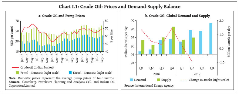
| Table I.2: Baseline Assumptions for Near-Term Projections | | Variable | April 2017 MPR | Current (October 2017) MPR | | Crude oil (Indian Basket) | US$ 50 per barrel during FY 2017-18 | US$ 55 per barrel during 2017-18: H2 | | Exchange rate | ₹65/US$ | Current level | | Monsoon | Normal for 2017 | 5 per cent below LPA | | Global growth | 3.4 per cent in 2017 3.6 per cent in 2018 | 3.5 per cent in 2017 3.6 per cent in 2018 | | Fiscal deficit | To remain within BE 2017- 18 (3.2 per cent of GDP) | To remain within BE 2017- 18 (3.2 per cent of GDP) | | Domestic macroeconomic/ structural policies during the forecast period | No major change | No major change | Notes: 1. The Indian basket of crude oil represents a derived numeraire comprising sour grade (Oman and Dubai average) and sweet grade (Brent) crude oil processed in Indian refineries in the ratio of 72:28.
2. The exchange rate path assumed here is for the purpose of generating staff’s baseline growth and inflation projections and does not indicate any ‘view’ on the level of the exchange rate. The Reserve Bank is guided by the need to contain volatility in the foreign exchange market and not by any specific level of/band around the exchange rate.
3. Global growth projections are from the World Economic Outlook (January 2017 and July 2017 updates), International Monetary Fund (IMF).
4. BE: Budget estimates.
5. LPA: Long period average (average rainfall during 1951-2000). |
Fourth, the outlook for global growth and trade remains broadly unchanged from the April 2017 assessment, with some acceleration relative to 2016 for both AEs and emerging market and developing economies (EMDEs) (Chart I.2). During 2018, AEs are expected to lose some momentum, with fiscal policy in the US projected to be less expansionary than expected in April. In contrast, EMDEs are expected to sustain the recent pick-up in growth. Increases in international air freight and container port throughput along with the plateauing of export orders suggest that the world trade volume growth, after some strengthening in the third quarter of 2017, could moderate towards the end of the year.1 This could have implications for staff’s baseline outlook for external demand. I.1 The Outlook for Inflation The softness in headline inflation observed during April-June 2017 is projected to reverse in the coming months. First, the prices of food items, especially of vegetables – which declined sharply in Q1 (April-June) as against the typical seasonal firming up in these months – have started edging higher. Second, the Central Government has implemented the increase in HRA for its employees effective July 2017. Third, there was a broad-based rebound in the various underlying measures of inflation in July-August 2017, reversing in large part the softness seen during April-June. Inflation expectations of economic agents play a key role in shaping the actual outcome through wages and price-setting behaviour. Quantitative inflation expectations of urban households eased by 30-60 bps in the September 2017 round of the Reserve Bank’s survey from the June 2017 round.2 Respondent households expected inflation to be 7.2 per cent three months ahead and 8.0 per cent a year ahead. In terms of qualitative responses, however, the proportion of respondents expecting the general price level to increase by more than the current rate rose over both the three-month and the one year horizons (Chart I.3). 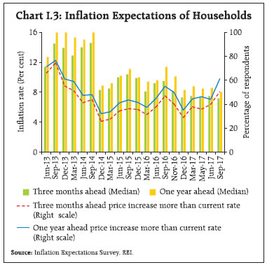 Manufacturing firms polled in the September 2017 round of the Reserve Bank’s industrial outlook survey expected some softening in inputs costs a quarter ahead, both for raw materials and staff costs.3 The respondents also expected some moderation in selling prices, indicating weak pricing power (Chart I.4). In the Nikkei’s purchasing managers’ survey for September 2017, firms in the manufacturing sector faced input and output price pressures from higher tax rates and prices of steel and petroleum products; firms in the services sector in August 2017 faced price pressures from higher tax rates. Professional forecasters surveyed by the Reserve Bank in September 2017 expected CPI inflation to pick up to 4.5 per cent by Q4:2017-18, with the ebbing away of favourable base effects (Chart I.5)4. Their medium-term inflation expectations (5 years ahead) remained unchanged at 4.3 per cent, while the longer-term inflation expectations (10 years ahead) rose by 10 bps to 4.1 per cent. 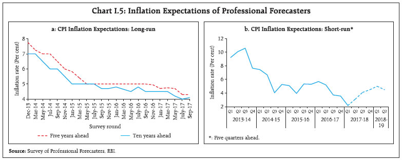 Taking into account the revised assumptions on initial conditions, signals from forward looking surveys and estimates from structural and other models, CPI inflation is projected to pick up from 3.4 per cent during August 2017 to 4.2 per cent in Q3:2017-18 and 4.6 per cent in Q4, reflecting the combined effects of unfavourable base effects, the upturn in food prices and the impact of the increase in the HRA (a statistical effect on the CPI index) announced by the Central Government (Chart I.6). The 50 per cent and the 70 per cent confidence intervals for inflation in Q4:2017-18 are 3.3-6.0 per cent and 2.6-6.8 per cent, respectively. For 2018-19, assuming a normal monsoon and no major exogenous shocks, structural model estimates indicate that inflation is expected to increase from 4.6 per cent in Q1 to 4.9 per cent in Q3 and then soften to 4.5 per cent by Q4:2018-19 as the statistical impact of the Central Government’s HRA enhancement fades. The 50 per cent and the 70 per cent confidence intervals for Q4:2018-19 are 2.7-6.5 per cent and 1.7- 7.5 per cent, respectively. 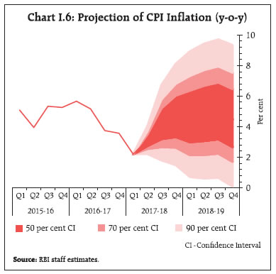 There are upside as well as downside risks to these baseline forecasts. The major upside risks emanate from the expected increases in salaries and allowances by State Governments; the possible fiscal slippages due to farm loan waivers by some States and potential stimulus measures by the Central Government (Box I.1); short-term uncertainty around the GST impact; and the expected decline in the production of kharif foodgrains. In terms of downside risks, adequate food stocks and effective supply management measures by the government could keep food inflation lower than expected and pull down headline inflation below the baseline. Box I.1: Farm Loan Waivers, Fiscal Stimulus and Inflation Five States – Maharashtra, Uttar Pradesh, Punjab, Karnataka and Rajasthan – have announced farm loan waivers in 2017-18 so far. Two of these states – Uttar Pradesh and Punjab – have made provisions for the likely increase in expenditure in their budgets for 2017- 18. During 2014-2016, three States – Andhra Pradesh, Telangana, and Tamil Nadu – had announced farm loan waivers aggregating ₹470 billion, but staggered over five years. There are reports of a few more States considering farm loan waivers. Furthermore, against the backdrop of the growth slowdown, there are reports that the Central Government might undertake policy actions to provide a boost to growth. Slowing growth could also have some adverse impact on tax revenues. The Central Government’s fiscal deficit could potentially widen on account of these factors. Taking these developments into considerations, the combined (Centre plus States) fiscal deficit to GDP ratio may increase by around 100 bps in 2017-18. Higher fiscal deficits per se can lead to an increase in inflation expectations and actual inflation (Catao and Terrones, 2005). Moreover, budget constraints might force some of the States to reduce their capital expenditure. If capital/infrastructural constraints are binding, a reduction in capital expenditure may turn out to be inflationary as costs – including time value/ opportunity cost of delays and material damages – go up as a result of capacity restraints becoming even more acute and due to attendant “congestion charges”. Higher market borrowings on the back of higher deficits can also put upward pressure on borrowing costs for the Centre and the States, which could spill over to the broader economy. Empirical assessment suggests that: (a) there exists a long-run relationship between fiscal deficits and inflation in India; (b) causality runs from fiscal deficits to inflation; and (c) the impact of fiscal deficits on inflation is non-linear, i.e., higher the initial levels of the fiscal deficit and inflation, higher is the impact of an increase in the fiscal deficit on inflation (Mitra et al., 2017) (Chart A).5 With the combined fiscal deficit budgeted at 5.9 per cent for 2017-18, empirical estimates suggest that an increase in the fiscal deficit to GDP ratio by 100 bps could lead to a permanent increase of about 50 bps in inflation. References: Catao, L.A. and M.E. Terrones (2005), “Fiscal Deficits and Inflation”, Journal of Monetary Economics, 52(3), 529-554. Mitra, P., I. Bhattacharyya, J. John, I. Manna and A.T. George (2017), “Farm Loan Waivers, Fiscal Deficit and Inflation”, Mint Street Memo No.5, Reserve Bank of India. Pesaran, M.H., Y. Shin and R.J. Smith (2001), “Bounds Testing Approaches to the Analysis of Level Relationships”, Journal of Applied Econometrics, 16(3), 289-326. | I.2 The Outlook for Growth The April 2017 MPR had projected an acceleration in real GVA for 2017-18 on the back of (a) a recovery in discretionary spending spurred by the pace of remonetisation; (b) the reduction in banks’ lending rates on fresh loans brought about by demonetisation-induced liquidity; (c) the growth stimulating proposals in the Union Budget 2017-18; (d) a normal south-west monsoon; and (e) an improvement in external demand. Stressed balance sheets of banks and the possibility of higher global commodity prices were seen as downside risks to growth prospects. Some of these expectations have materialised, whereas the recovery in discretionary and investment spending has been weaker than expected and kharif foodgrains production is expected to be lower than last year in view of the shortfall and irregular rainfall during the south-west monsoon this year. The uncertainty about the implementation of GST also appears to have had some impact on economic activity, although it is expected to be offset by productivity-enhancing effects in the medium- and long-run. Consumer confidence dipped in the September 2017 round of the RBI’s survey on declining optimism about prospects of income and employment a year ahead (Chart I.7).6 Overall optimism in the manufacturing sector for the quarter ahead improved in the September round of the RBI’s industrial outlook survey on account of better prospects for production, order books, capacity utilisation, exports and profit margins, even as the current assessment dropped further (Chart I.8). Surveys conducted by other agencies indicate a dip in business confidence over the previous round (Table I.3). In the Nikkei’s purchasing managers’ survey, firms in the manufacturing sector (September 2017) and the services sector (August 2017) were optimistic about future output prospects. | Table I.3: Business Expectations Surveys | | Item | NCAER Business Confidence Index (July 2017) | FICCI Overall Business Confidence Index (August 2017) | Dun and Bradstreet Composite Business Optimism Index (June 2017) | CII Business Confidence Index (September 2017) | | Current level of the index | 136.0 | 66.1 | 72.1 | 58.3 | | Index as per previous Survey | 139.5 | 68.3 | 78.9 | 64.4 | | % change (q-o-q) sequential | -2.5 | -3.2 | -8.6 | -9.5 | | % change (y-o-y) | 9.4 | -1.8@ | -13.3 | 0.5 | Notes: 1. NCAER: National Council of Applied Economic Research.
2. FICCI: Federation of Indian Chambers of Commerce and Industry.
3. CII: Confederation of Indian Industry.
@: Change over the October 2016 round. | 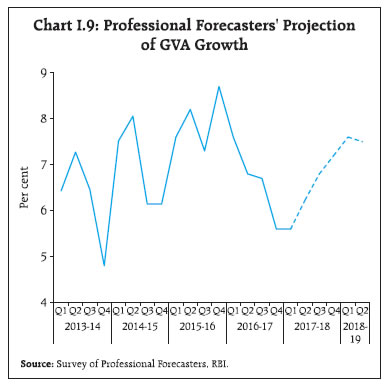
| Table I.4: Reserve Bank’s Baseline and Professional Forecasters’ Median Projections | | (Per cent) | | | 2017-18 | 2018-19 | | Reserve Bank’s Baseline Projections | | | | Inflation, Q4 (y-o-y) | 4.6 | 4.5 | | Real Gross Value Added (GVA) Growth | 6.7 | 7.4 | | Assessment of Professional Forecasters@ | | | | Inflation, Q4 (y-o-y) | 4.5 | 4.5# | | GVA Growth | 6.6 | 7.4 | | Agriculture and Allied Activities | 3.2 | 3.0 | | Industry | 4.8 | 7.0 | | Services | 8.1 | 8.7 | | Gross Domestic Saving (per cent of GNDI) | 31.2 | 32.3 | | Gross Fixed Capital Formation (per cent of GDP) | 26.5 | 27.6 | | Credit Growth of Scheduled Commercial Banks | 8.0 | 10.0 | | Combined Gross Fiscal Deficit (per cent of GDP) | 6.5 | 6.0 | | Central Government Gross Fiscal Deficit (per cent of GDP) | 3.2 | 3.0 | | Repo Rate (end period) | 6.00 | 6.00# | | Yield on 91-days Treasury Bills (end period) | 6.0 | 6.1 | | Yield on 10-years Central Government Securities (end period) | 6.7 | 6.9 | | Overall Balance of Payments (US $ billion.) | 30.0 | 25.0 | | Merchandise Export Growth | 6.5 | 7.9 | | Merchandise Import Growth | 11.5 | 9.5 | | Current Account Balance (per cent of GDP) | -1.5 | -1.8 | @: Median forecasts; GNDI: Gross National Disposable Income.
#: Forecast for Q2:2018-19.
Source: RBI staff estimates; and Survey of Professional Forecasters (September 2017). | 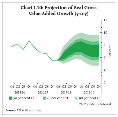 In the September round of the RBI’s survey, professional forecasters expected real GVA growth to pick up from 5.6 per cent in Q1:2017-18 to 7.2 per cent in Q4:2017-18 and to 7.5 per cent in Q2:2018-19, led by improvement in industry and services sector activity (Chart I.9 and Table I.4). Taking into account the outturn in the first half, the baseline assumptions, survey indicators and model forecasts, real GVA growth is projected at 6.7 per cent for 2017-18 – 6.4 per cent in Q2, 7.1 per cent in Q3 and 7.7 per cent in Q4 – with risks evenly balanced around this baseline path. For 2018-19, structural model estimates indicate that real GVA may grow by 7.4 per cent, assuming a normal monsoon, fiscal consolidation in line with the announced trajectory, and no major exogenous/policy shocks (Chart I.10). Dynamic Stochastic General Equilibrium (DSGE) models are workhorse tools for policy analysis by a number of central banks. In the RBI, efforts are underway to develop such a model to enrich analytical inputs for the conduct of future monetary policy (Box I.2). Box I.2: Towards a Prototype Dynamic Stochastic General Equilibrium (DSGE) Model for India Built on microeconomic foundations, DSGE models emphasise agents’ inter-temporal choice and assign a central role to agents’ expectations around the determination of macroeconomic outcomes. These models are able to generate outcomes from policy simulations (or counterfactuals) that are not explicitly susceptible to the Lucas (1976) critique of traditional macro-econometric models using reduced-form representations that may not be robust to shifts in the underlying economic structure induced by changes in policy. Given the general equilibrium nature, the DSGE models can capture the interplay between policy actions and agents’ behaviour (Sbordone et al, 2010). The earliest DSGE model, representing an economy without distortions, was the real business cycle model that focused on the effects of productivity shocks (Kydland and Prescott, 1982). Since then, there has been considerable improvement in specification and estimation techniques. Current DSGE models embody a wider set of distortions and shocks than earlier generation efforts (Christiano et al., 2005; Smets and Wouters, 2007). Several central banks, both in AEs and EMEs – Bank of Canada; Bank of England; European Central Bank; Central Bank of Chile to name a few – have developed such models for policy analysis and employ them extensively to evaluate alternative policy scenarios and instrument choices. A prototype New Keynesian DSGE model for India would need to be calibrated to country specific conditions. Drawing on Ireland (2004), the economy is hypothesised to be inhabited by a representative household which maximises a lifetime expected utility function, subject to an inter-temporal budget constraint. The felicity function7 depends on consumption (C) and labour (l) supplied to the intermediate goods producing sector. The first-order condition of household optimisation consists of (i) the Euler equation which relates the real interest rate to the inter-temporal marginal rate of substitution; and (ii) an inter-temporal optimality condition linking the real wage to the marginal rate of substitution between leisure and consumption. policy shock. Equations (1)-(5), along with the marketclearing condition, constitute the system of equations which can be solved using standard DSGE methods.9 The model parameters can be calibrated to various Indian studies (Patra and Kapur, 2012). In this prototype model, it is possible then to run counter-factual exercises, e.g., simulate the economy wide effect of an expansionary monetary policy a la the reduction in the policy repo rate as in the third bi-monthly monetary policy statement of August 2, 2017. An expansionary monetary policy shock reduces interest rate and raises output, consumption and inflation, as illustrated in Chart B. References: Christiano, L.J., L. Eichenbaum, and C.L. Evans (2005), “Nominal Rigidities and Dynamic Effects of a Shock to Monetary Policy”, Journal of Political Economy, 113 (1), 1-45. Ireland, P. (2004), “Technology Shocks in the New Keynesian Model”, NBER Working Paper, No.10309, February. Kydland, F.E. and E.C. Prescott (1982), “Time to Build and Aggregate Fluctuations”, Econometrica: Journal of Econometric Society, 50, 1345-1370. Lucas, R. (1976), “Econometric Policy Valuation: A Critique”, In Carnegie-Rochester Conference Series on Public Policy, Vol.1, 19-46, North Holland. Mumtaz, H. and F. Zanetti (2013), “The Impact of the Volatility of Monetary Policy Shocks”, Journal of Money, Credit and Banking, 45(4), 535-558. Patra, M.D. and M. Kapur (2012), “Alternative Monetary Policy Rules for India”, IMF Working Paper, WP/12/118. Sbordone, A.M., A. Tambalotti, K. Rao and K. Walsh (2010), “Policy Analysis using DSGE Models – An Introduction”, FRBNY Economic Policy Review, October, 23-43. Smets, F. and R. Wouters (2007), “Shocks and Frictions in US Business Cycles”, ECB Working Paper Series, No.722, February. | I.3 Balance of Risks The baseline projections of growth and inflation are inter alia conditional on the assumptions set out in Table I.1. A caveat is that the baseline growth and inflation trajectories do not incorporate the impact of the likely increases in pay and allowances by State Governments for their employees. This section makes an assessment of the balance of risks around the baseline projections from a set of plausible alternative scenarios. (i) International Crude Oil Prices In the baseline forecasts, the crude oil (Indian basket) price is assumed to average around US$ 55 per barrel in the second half of 2017-18 on the expectation that the global oil supply would be sufficient to meet increasing global demand. However, supply disruptions due to geo-political developments with oil demand remaining robust could push crude oil prices higher. The upward pressures on oil prices could, however, get mitigated by the increased production of shale gas in response to higher prices. Assuming that crude oil prices reach US$ 65 in the second half of 2017-18 in this scenario, inflation could be higher by about 30 bps in 2017-18. Real GVA growth could weaken by around 15 bps in 2017-18 due to the direct impact of higher input costs as well as spillovers from lower world demand. If, in contrast, crude oil prices soften below the baseline due to oversupply by the Organisation of the Petroleum Exporting Countries (OPEC) and/or weaker than anticipated global demand and in particular, fall to around US$ 50, inflation may moderate by about 15 bps, with a boost to real GVA growth of around 5-10 bps above the baseline in 2017-18 (Charts I.11 and I.12). 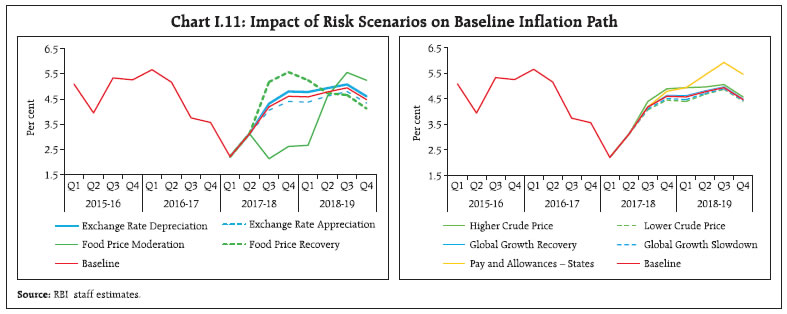 (ii) Global Demand Global demand is expected to be higher in 2017 and 2018 in the baseline scenario with both upside and downside risks to the outlook. On the downside, the expected demand boost from expansionary US fiscal policy may not materialise, given recent developments in the US. In China, growth has remained resilient, but concerns over its sustainability remain in view of the large overhang of debt. Persisting disconnect between market participants’ assessment and that of the US Federal Open Market Committee (FOMC) over the pace of US monetary policy normalisation could trigger volatility in financial markets, especially in view of stretched market valuations. The ensuing tightening of global financial conditions in a milieu of inward-looking protectionist tendencies could amplify downside risks, especially for EMEs. Assuming global growth turns out to be 50 bps below the baseline, domestic growth and inflation could fall below the baseline forecasts by around 20 bps and 10 bps, respectively. However, reduced political risks in the euro area could lead to a more sustained and stronger cyclical rebound, providing a boost to global growth. Assuming that global growth is higher by 25 bps, real GVA growth and inflation could turn out to be around 10 bps and 5 bps, respectively, above the baseline. 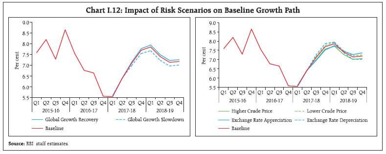 (iii) Exchange Rate The exchange rate of the Indian rupee has exhibited two-way movements vis-à-vis the US dollar during the first half of 2017-18. Going forward, the normalisation of monetary policy in the US (and possibly other central banks in AEs) and protectionist policies of major AEs and EMEs could lead to some volatility in the foreign exchange market and downward pressures on the exchange rate. A depreciation of the Indian rupee by around 5 per cent relative to the baseline could raise inflation by around 20 bps in 2017-18, while producing some positive impact on net exports and growth. On the other hand, in view of the robust growth prospects of the Indian economy in a cross-country perspective and the various initiatives to attract foreign direct investment, India is likely to remain an attractive destination for foreign investors and this could lead to an appreciation of the domestic currency. An appreciation of the Indian rupee by 5 per cent could soften inflation by around 20 bps but also deliver a negative impact of 10-15 bps on real GVA growth. (iv) Food Inflation The substantial softening of headline inflation in the first quarter of 2017-18 reflected the absence of the usual seasonal pick up in food prices in the post-winter period, especially pulses and vegetables. These food price dynamics may have both structural and cyclical elements, although it is difficult to disentangle them at this juncture. If the softening in food inflation observed since the second half of 2016 is largely structural, then the momentum in food prices in the rest of 2017-18 could be negligible and headline inflation could be below the baseline by up to 2 percentage points. If however, low food inflation turns out to be largely cyclical, food prices are likely to revert to trend. Assuming that the momentum in the food prices in the coming months is in line with the average of the past five years, headline inflation may turn out to be 100 bps above the baseline. (v) Pay and Allowances – Implementation by States The impact of increased salaries and pensions of Central Government employees in 2016 and the implementation of HRA effective July 2017 has been embedded in the baseline forecasts. Assuming that State Governments implement a similar order of increase in their pay and allowances, CPI inflation could go up to 100 bps above the baseline on account of the direct statistical effect of higher house rents with possible indirect effects emanating from higher demand and increase in inflation expectations. (vi) Fiscal Slippage As noted earlier, there are upside risks to the Central Government’s fiscal deficit from possible measures to provide a boost to domestic demand and from lower tax revenues. Assuming that the Central Government’s fiscal deficit/GDP ratio widens by 50 bps in 2017-18, inflation could be around 25 bps above the baseline. To conclude, the growth outlook is expected to improve in the second half of 2017-18, although it could be weighed down by still sluggish investment and export activity. Higher food prices and the increase in house rent allowances by the Central Government for its employees are expected to result in an increase in headline inflation in the second half of 2017-18. There are upside risks to the inflation outlook from (i) the lower kharif foodgrains output; (ii) farm loan waivers by some State Governments and possibility of Central Government stimulus; and (iii) the implementation of higher pay and allowances by the State Governments for their employees, which will impact the baseline projections of growth and inflation as they materialise.
II. Prices and Costs Consumer price inflation fell sharply in the first quarter of 2017-18, driven down by a collapse in food inflation and a marked moderation in inflation in other components. The trajectory reversed in July and August as vegetable prices spiked and prices of other goods and services firmed up. Input costs tracked movements in international commodity prices, while wage growth in the organised and rural sectors firmed up modestly. The MPR of April 2017 had projected consumer price index (CPI) inflation1 to increase to 4.2 per cent in Q1:2017-18 and further to 4.7 per cent in Q2 on the expectation that the compression imposed by demonetisation on perishable food prices would wane, and the usual seasonal uptick that characterises pre-monsoon months would take over. In the event, inflation developments in the first half of 2017- 18 were foreshadowed by the prolonged impact of food supply shocks. Consequently, actual inflation outcomes were pushed much below their projected path. First, food prices sank into deflation in May and June 2017. Second, crude prices fell in April, remaining soft and range-bound in ensuing months; combined with an appreciating exchange rate, this resulted in a sharp disinflation in petrol and diesel prices in the early part of 2017-18. In the fuel group, liquefied petroleum gas (LPG) prices declined in the first quarter of 2017-18, tracking international prices. Third, inflation excluding food and fuel also eased significantly in Q1:2017-18, pending price revisions ahead of goods and services tax (GST) implementation. The cumulative impact was that headline inflation plunged to 2.2 per cent in Q1:2017-18 and 2.9 per cent in the first two months of Q2 – significantly lower than the assessment made at the time of the April MPR. Although these forces continue to drive a wedge between actual and projected inflation in terms of levels, a directional alignment is gradually occurring since July (Chart II.1a). Large and unanticipated supply shocks have produced at least two systematic deviations of actual and projected inflation in terms of the new index (Chart II.1b). Both capture significant underlying shifts in demand-supply balances in key inflation-sensitive goods and services, which should have warranted policy responses of a scale and range beyond the narrow remit of monetary policy. II.1 Consumer Prices After the January 2017 trough, consumer price inflation increased for two months in succession to reach 3.9 per cent in March. Thereafter, inflation started declining sharply to reach a historic low of 1.5 per cent in June (Chart II.2), driven by the sequential decline in the momentum of food prices and the overwhelming downward pull of favourable base effects that took the prices of food items down into a deflation of (-)1.2 per cent by June. This dramatic decline was accentuated by the dampening of the usual seasonal spikes in prices of vegetables that typically manifest ahead of the onset of the monsoon. Inflation excluding food and fuel also declined sharply from 5 per cent in March to 3.8 per cent by June, after a long hiatus of stickiness. The sharp disinflation during April to June 2017 in prices of goods and services constituting this category came from favourable base effects offsetting positive but weak momentum (Chart II.3a, b and c). 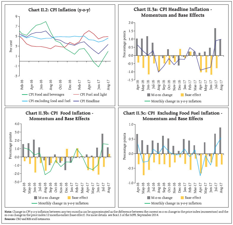 The sharp disinflation in CPI from 3.7 per cent in the second half of 2016-17 to 2.5 per cent in the first half of this year impacted the inflation distribution. The moderation in the central tendency of the distribution was also accompanied by an increase in kurtosis and a considerable negative skew, as against a positive skew during the corresponding period a year ago (Chart II.4). On a seasonally adjusted basis, prices of most items registered increases and the diffusion indices2 for goods, services and the overall CPI were well above 50 (Chart II.5). In July and August 2017, the incidence of delayed spikes in prices of vegetables within an overall firming up of prices of goods and services in the run up to the GST implementation reversed the trajectory of headline inflation and diffusion indices rose sharply, indicating renewed broad-basing of price pressures.
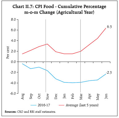
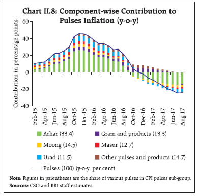
II.2 Drivers of Inflation A historical decomposition3 of inflation shows that large supply shocks dominated the disinflation of the first half of 2017-18, contributing 3.6 percentage points to it. This confirms the vulnerability of the Indian economy to exogenous shocks, viz., oil prices, and disruptions impacting the agriculture sector in spite of the diversification and weather proofing of the agricultural sector sought to be achieved by policy interventions over time. These developments may warrant a re-appraisal of the scope and quality of food management strategies that seem prone to failure in the face of shocks in either direction. In the past too, supply shocks, of which large one-sided deviations of inflation from projections are merely a symptom, drove disinflation episodes. The softening of oil prices in conjunction with exchange rate appreciation and the negative output gap, possibly due to weak credit growth, also contributed to the disinflation (Chart II.6a). Drilling down into granular constituents, non-durable goods, which account for 66 per cent of the CPI basket and include items such as petrol and diesel in addition to food items, were the main drivers of the disinflation. The contribution of services, on the other hand, remained broadly unchanged. The reversal in July and August was driven by inflation in non-durables which rebounded, led by food prices (Chart II.6b). Turning to a disaggregated analysis of food inflation, this recent experience with a disinflation episode yields several lessons that should inform the setting of macroeconomic policies going forward in order to pre-empt widespread distress in the farm economy or at least, to mitigate it. The precipitous decline in food prices appears to have overwhelmed supply management efforts, despite the fact that the downshift in momentum commenced as early as the second half of 2016-17 and continued well into the first quarter of 2017-18, affording lead time for course corrections. This decline in food prices during August 2016 to June 2017 [(-)2.3 per cent] was in stark contrast to the pattern of the last five years (2011-12 to 2015- 16) when food prices increased at an average annual rate of 6.3 per cent (Chart II.7). Two factors stand out in this experience as noteworthy. First, the unusually low and delayed seasonal upticks in vegetables prices coincided with larger than usual arrivals in mandis which did not get contemporaneously picked up by agri-information alerts. Also highly unusual were the spillovers to prices of vegetables other than the usual suspects – potatoes; onions; tomatoes – indicating the extent of dislocation caused by oversupply, since other vegetables do not typically exhibit significant seasonal swings. Second, there was a massive deflation in respect of prices of pulses – (-)24.6 per cent by July-August 2017 contributed by all items in the pulses group (Chart II.8). It was preceded, however, by a steady and sizable disinflation from the second half of 2015-16 which should have flashed in lead monitors of the pulses economy. In the absence of corrective action, the combination of augmented availability and inadequate procurement/marketing operations yielded a supply glut with which food supply management logistics failed to cope. 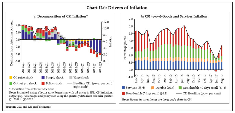
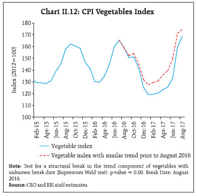
 As regards specific components in the food category, pulses constitute 2.4 per cent of the CPI and 5.2 per cent of the food category. The decline in prices of pulses contributed (-)1.4 percentage points to the food deflation during May and June and (-)0.7 percentage points to headline disinflation (Chart II.9). Historically, domestic production and imports of pulses have consistently lagged behind the level of domestic demand, resulting in inflationary pressures on the headline. Drawing upon this experience, the Government put in place several measures to augment supply during 2016-17, which inter alia included increasing the minimum support prices (MSPs) to incentivise farmers to increase acreage (MSP for kharif and rabi pulses increased in the range of 7.7-9.2 per cent and 14.3-16.2 per cent, respectively, in 2016-17); continuing zero import duty on pulses to augment domestic availability of pulses at reasonable prices (import duty of 10 per cent was imposed on tur in March 2017 to prevent prices from falling below MSPs); restricting exports (tur, moong and urad dal have been made free for exports, effective September 15, 2017); creating buffer stocks of pulses for the first time through involvement of agencies such as the Food Corporation of India (FCI), the National Agricultural Cooperative Marketing Federation of India Ltd. (NAFED), and the Small Farmers’ Agri Business Consortium (SFAC); discouraging hoarding by putting stock limits on pulses for traders (which were lifted in May 2017); and taking measures for revitalising the agriculture sector in general.4  With the domestic availability of pulses (domestic production and imports) increasing to 29.6 million tonnes in 2016-17 from 22.2 million tonnes in 2015- 16, the prices of pulses declined below their long-term trend as well as the MSPs in several mandis (Charts II.10a, b and c). This reflected the large gap in procurement relative to supply and the unanticipated shock to farmers’ expectations on price support. In the case of vegetables, prices fell significantly since August 2016, with statistical tests suggesting a trend break5 that altered their evolution incipiently under the cover of the transitory effects of demonetisation. A sequence of positive shocks brought about this sub-trend deviation. What started off as the reversal of the summer spike in August was followed by the sharp and more than seasonal winter price correction. Firesales post demonetisation set the stage for a plunge in the prices of other vegetables (cabbage; cauliflower; palak/other leafy vegetables; brinjal; gourd, peas and beans) during November-December 2016, which usually exhibit little seasonality, as stated earlier. Finally, there has been an unusually soft pickup in vegetable prices during the early months of 2017 (Charts II.11 and II.12). This was due to large arrivals of key vegetables during these months. These developments underscore the need for high frequency data and monitoring of prices, mandi arrivals, supply-demand balances and stock positions, especially with respect to horticulture. 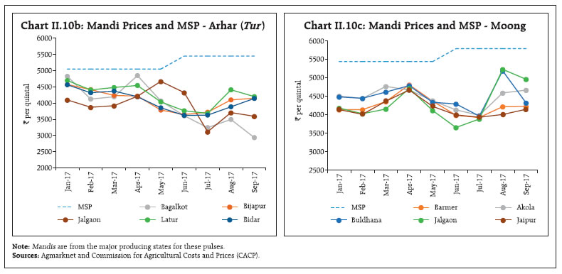 In Q2 so far, food inflation has edged up on the back of a sharp rise in vegetables prices, driven by a spike in tomato and onion prices (Chart II.11). In the case of tomatoes, sudden price movements propelled inflation in the item from (-)40.8 per cent in June 2017 to 49.9 per cent in July and further to 94.0 per cent in August. This was mainly on account of supply disruptions due to farmers’ agitations in Maharashtra in June and adverse weather conditions in important production centres. In early August, upside pressures also built up in onion prices, pushing onion inflation to 49.3 per cent in August from (-)10 per cent in July, reportedly due to damage caused by July rains and large procurement by a few State Governments. The sharp increase in these prices in retail markets reflects a statistically significant increase in margins6 in Q2:2017-18. Further analysis based on CPI regional prices data suggests that there is no significant difference in the changes in vegetable prices in urban and rural areas – the spike in vegetable prices has uniformly impacted rural and urban India.7 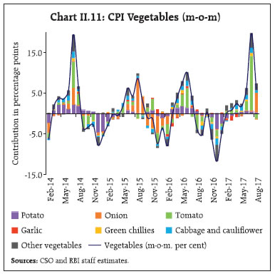
 Among other food items, prices of spices moved into deflation territory since June 2017 on account of a fall in prices of chillies, dhania and black pepper. As per the 3rd advance estimates of the Ministry of Agriculture, production of spices recorded a growth of 17.4 per cent in 2016-17, up from 14.4 per cent a year ago. Sugar inflation, which was in double digits during 2016-17 (averaging 20 per cent), also eased in 2017-18 so far (up to August), largely due to measures facilitating imports and on expectations of higher domestic production. inflation in prices of animal proteins and milk has declined as momentum was weak and base effects favourable. Cereal inflation remained low and moved with a softening bias due to higher availability – production was higher and stocks were up by 5.09 million tonnes.8 Import duty on wheat that was reduced to zero in December 2016 was re-imposed in March 2017. In the fuel and light group, inflation picked up at the start of the financial year but softened transiently in May-June before resuming an upturn in July and August. The decision to allow oil marketing companies (OMCs) to raise subsidised kerosene and LPG prices in a calibrated manner has enhanced the responsiveness of prices of domestic household fuel items to international price benchmarks. The contribution of electricity to overall fuel inflation remained more or less unchanged in H1:2017-18 in relation to the corresponding period of last year, while that of firewood moderated (Chart II.13). Growth in electricity generation9 decelerated during Q1:2017- 18 to 5.3 per cent (from a robust base of 10 per cent last year) on account of subdued performance of the manufacturing sector; though it has accelerated significantly in the months of July and August with a growth rate of 7.5 per cent (from 2.1 per cent last year) with reports of surge in rural demand for irrigation. The long-term thermal-based power tariff through power purchasing agreements (PPA) by distribution companies (DISCOMs), the dominant source of electricity, has remained broadly unchanged. However, spot price of electricity reported on energy exchanges, which was broadly the same as last year till April 2017, have started rising from May 2017 onwards. 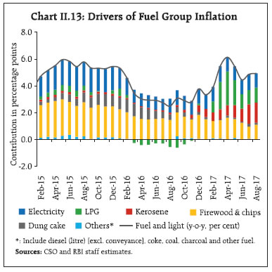 Turning to the underlying inflation dynamics, CPI inflation excluding food and fuel edged down by 120 basis points during the year up to June. The softness in prices of petrol and diesel within the transport and communication group contributed substantially to the observed moderation in Q1 (Chart II.14). Excluding petrol and diesel prices from this category too, inflation moderated (Chart II.15). The sudden and sharp decline in inflation excluding food, fuel, petrol and diesel in Q1:2017-18 was driven by goods as well as services. Among goods, much of the moderation was in prices of personal care and effects due to a fall in the rate of change of domestic gold prices in tandem with international prices. inflation in respect of goods within the health sub-group and clothing also eased, pending price revisions held back ahead of GST, while clearance sales depressed inflation in the case of clothing (Chart II.16a). 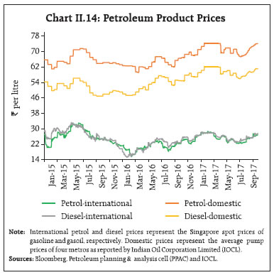
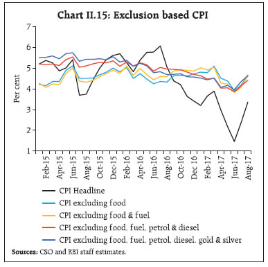 Services inflation eased during Q1:2017-18 in a broad-based manner. inflation in respect of education services moderated significantly, possibly on account of the revised school fee payment cycle for central school boards for the academic year. Lower inflation was recorded in transportation fares as fuel prices remained range-bound, coupled with food inflation – a major determinant of the cost of living – being lower than in the recent past. Prices of mobile communication expenses eased significantly, triggered by pricing war in the telecommunication sector. Housing inflation also moderated in Q1, reflecting lower rates of increase in rentals (Chart II.16b). Thereafter, in July and August, there was a broad based pickup in CPI inflation excluding food and fuel. inflation in transport and communication registered sharp increase driven by petrol and diesel (Chart II.14). Household goods and services; pan, tobacco and intoxicants; health; recreation; and clothing and footwear sub-groups also rose. This partly reflected the hike in the service tax rate under GST and the impact of GST on certain goods, especially packaged/ processed food; clothing and footwear; and recreation and amusement services. Housing inflation reversed with the implementation of house rent allowance (HRA) increases by the Centre from July. As a result, all other exclusion based measures also registered a pickup in Q2 so far (Chart II.15). The GST was rolled out in July 2017. The assessment at the current juncture is that price changes are not likely to have any material impact on headline inflation. However, in case the price increases show downward rigidity due to uncertainty in GST implementation, inflationary impact may emerge (Box II.1). 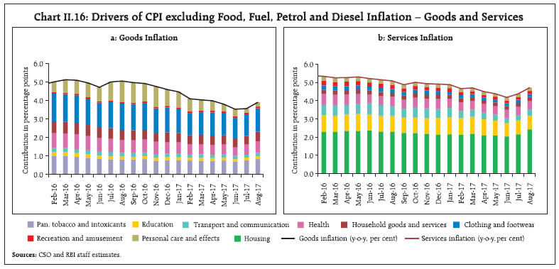 Box II.1: Impact of GST on CPI inflation The goods and services tax (GST) has been implemented from July 1, 2017 with the GST Council broadly approving a five-tier rate structure, viz., 0 per cent for commodities such as fruits, vegetables, milk, handloom, select agricultural implements and newspapers; 5 per cent for coal, sugar, tea, coffee, edible oil, economy air fares among others; 12 per cent for select processed foods among others; 18 per cent for non-durables and most of the services; and 28 per cent for most consumer durable goods and recreation services. Non-processed food items, education, health care, real estate, electricity and fuel items like petrol and diesel are exempted from the GST. A rate of 3 per cent has also been specified for gold. The major indirect taxes that were subsumed under the GST include the excise duty, the service tax, Central sales tax and State value added tax (VAT). In order to arrive at the direct impact of the GST structure on the CPI, a comparison of the existing excise and State VAT/sales tax rates on CPI items vis-à-vis the GST rate structure is in order. Almost half of the CPI basket comprises food items that attracted zero excise and sales tax and they continue to be taxed at the zero rate under the new GST rate structure. Furthermore, petrol and diesel are outside the purview of the GST on which the existing taxation system (VAT and central excise duty) will continue. Hence, the impact of GST on CPI stems mainly from the tax rate differentials in respect of the remaining elements of the CPI basket. From an item level mapping of the earlier tax rates and the new GST rate structure, it is observed that among the major sub-groups, much of the increase in prices post-GST is estimated to occur in prepared meals, clothing and footwear and other sub-groups dominated by services such as recreation and amusement. The increase in prices of these items is to a large extent likely to be offset by declines in post- GST goods prices – particularly those in the household goods and services sub-group and personal care and effects as well as in select food sub-groups such as spices and pulses. Overall, taking into account the weighted contribution of the changes in the major sub-groups, CPI prices could increase by around 10 basis points on account of the new GST rate structure (Chart 1). As such, it is not expected to have any significant impact on CPI inflation. Estimates by other agencies also point to a muted impact of the new GST rate structure on CPI inflation10. However, as noted in the October 2016 MPR (Box II.I: inflation Impact of GST – Cross Country Evidence), the cross-country experience shows a one-off increase in prices in the first year following the introduction of GST. This is likely on account of firms choosing to increase prices initially in response to the uncertainties surrounding the implementation of a new tax system and its impact on business processes. Similar behaviour by firms in India in response to GST implementation could result in some upside risk to the inflation assessment presented here. A dip stick survey was conducted by the Reserve Bank in select cities to assess the impact of implementation of GST on prices of eighteen commodities. The survey results suggest that the weighted average price of these commodities, with a weight of around 10.0 per cent in the CPI basket, is likely to have gone up by 0.8 per cent including the regular price change. Post-GST price rise is witnessed in textiles, footwear and utensils, whereas prices of two-wheelers and some fast moving consumer goods (FMCG) items have moderated. In case prices of commodities that have gone up show downward rigidity, the weighted average price increase could be higher at 1.5 per cent [Table 1, Column (4)]. | Table 1: Impact of GST on Inflation Based on Survey Conducted by the RBI in mid-September 2017 | | Items | Weights in CPI basket | Per cent change | Max [0, Per cent change] | | (1) | (2) | (3) | (4) | | Biscuits | 0.9 | 3.9 | 3.9 | | Ice Cream | 0.0 | 7.6 | 7.6 | | Prepared Sweets | 0.6 | 2.5 | 2.5 | | Tea | 1.0 | -1.5 | 0.0 | | Edible Oil | 3.0 | 0.1 | 0.1 | | Shirts | 0.6 | 3.7 | 3.7 | | Sarees | 0.9 | 5.7 | 5.7 | | Leather Shoes | 0.2 | 4.6 | 4.6 | | Rubber / PVC Footwear | 0.3 | 3.6 | 3.6 | | Televisions | 0.2 | 1.0 | 1.0 | | Refrigerators | 0.1 | 0.6 | 0.6 | | Stainless steel utensils | 0.2 | 2.3 | 2.3 | | Pressure-cooker/ Pan | 0.0 | 1.9 | 1.9 | | Electric-bulb / Tubelight | 0.2 | 0.8 | 0.8 | | Washing-soap / Powder | 0.9 | -2.3 | 0.0 | | Motorcycle / Scooter | 0.8 | -2.9 | 0.0 | | Hair-oil / Shampoo | 0.5 | 0.9 | 0.9 | | Toothpaste | 0.4 | -4.1 | 0.0 | | Total | 10.4 | 0.8 | 1.5 | | Source: RBI survey. | | Other Measures of inflation In May 2017, the base year of wholesale price index (WPI) was revised from 2004-05 to 2011-12 to align it with the base year of other macroeconomic indicators such as gross domestic product (GDP) and the index of industrial production (IIP). The revision in the base year is also intended to capture structural changes in the economy and to improve the quality, coverage and representativeness of the index. In addition to an updated item basket, the revised WPI has included two new features in line with international best practices: (i) the use of the geometric mean for compilation of item-level indices; and (ii) the exclusion of indirect taxes from wholesale prices, thus bringing it conceptually closer to a producer price index. Reflecting these changes, headline WPI inflation in the new series declined by an average of one percentage point as compared with inflation calculated from the index with 2004-05 as base year during April 2013 to March 2017. 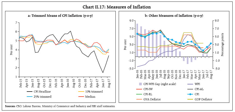 After peaking in February, WPI inflation fell sharply up to June, but ticked up again in July and August following a sharp pickup in food prices. Between April and July, CPI trimmed means11 have softened; however, in August these registered an increase. Median inflation, a particular case of the trimmed mean, also declined, averaging 4.2 per cent since March 2017 (Chart II.17a). inflation measured by sectoral consumer price indices continued to undershoot headline CPI inflation, reflecting inter alia the higher weight of food in the former. Changes in GDP and gross value added (GVA) deflators have moved along with WPI inflation since the beginning of the year (Chart II.17b). In July and August, the movement in WPI inflation was consistent with that of headline CPI and all sectoral CPIs. II.3 Costs Underlying cost conditions have largely co-moved with measures of inflation, with the pickup in the last quarter of 2016-17 turning out to be transient. Industrial and farm costs captured under the WPI eased significantly in Q1:2017-18 (Chart II.18). The fall in global crude oil prices and the easing of metal prices due to the slowdown of demand from China12, the world’s biggest metals consumer, also contributed to the significant decline in domestic farm and nonfarm input costs as they got passed on to inputs such as high speed diesel, aviation turbine fuel, naptha, bitumen, furnace oil and lube oils. In Q2, metal prices rose from the June trough, underpinned by expectations of strong global demand, particularly from China. However, prices moderated somewhat by end-September. 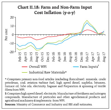 Among other industrial raw materials, domestic coal prices remained range-bound while prices of other inputs such as fibres, oil seeds and pulp either declined or moved with a softening bias; and among farm sector inputs, diesel prices declined sharply, tracking international prices. Prices of other agricultural inputs such as electricity, fertilisers, pesticides and tractors softened. Due to excess inventory, supply of fertiliser remained comfortable despite deceleration in production in Q1:2017-18 which softened prices. Tractor shipments decelerated to 8.0 per cent in Q1:2017-18 (12.1 per cent last year) largely due to destocking in the pre-GST period, with discounts imparting low momentum to prices. However, the decline in inflation in both farm inputs and industrial raw materials was arrested in the August prints as the prices of urea, high speed diesel and other minerals oil rose tracking international prices. Following the monsoon and the pickup in agricultural activity, demand for agricultural labourers remained strong in 2017-18. This was reflected in a modest increase in the rate of wage growth for rural agricultural labourers, a key determinant of farm costs (Chart II.19). In the organised sector, the decline in growth of unit employee costs in listed private sector companies in manufacturing during 2016-17 reversed to register an uptick in Q1:2017-18. However, unit employee costs for companies in the services sector continued to decline in a pattern that has set in since Q2:2016-17.13 Unit labour costs14 in the manufacturing sector continued to rise as staff cost growth outpaced the growth in value of production.15 The growth in the ratio of staff costs to value of production in the manufacturing sector accelerated modestly in the first quarter of 2017-1816 after declining for the last two quarters of 2016-17 (Chart II.20). The value of production for manufacturing companies declined (probably due to de-stocking undertaken by the companies with respect to pre-GST sales) and staff costs rose marginally. 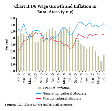 The cost of raw materials, based on responses of manufacturing firms covered in the Reserve Bank’s industrial outlook survey, remained high in Q1:2017- 18, albeit with some moderation in relation to the previous quarter, possibly reflecting softer commodity prices. Firms assessed that the cost of raw materials remained elevated in Q2 as well; however, their inability to increase selling prices suggests that pricing power is still weak. The manufacturing purchasing managers’ index (PMI) also suggest that the cost of raw materials remained high in Q1 and Q2:2017-18, but failed to impact selling prices in view of weak pricing power. In contrast, the services PMI reported a sharp pickup in prices charged in Q2 – the upward revision in prices likely reflecting higher tax rates under GST. 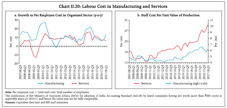 Globally, low inflation across AEs and EMEs is coexisting with a modest strengthening of demand. In India, uncertainty surrounds the path of inflation over the rest of the year. Overall inflation outcomes going forward will depend on the durability of the recent disinflation in food, given that base effects have turned unfavourable from August. Furthermore, there are likely headwinds from temporary price adjustments post-GST, the direct and second round impact of HRA increases (see MPR, April 2017, Chapter 1) and a recovery in demand in the second half of 2017-18 which would narrow the output gap. Consequently, the inflation trajectory is poised to firm up over the rest of the year. Finally, considerable upside risk to inflation stems also from the rather large scale of state level farm loan waivers and the reports of a likely fiscal stimulus (Chapter I, Box I.1).
III. Demand and Output Aggregate demand has been impacted by slowing consumption demand, still subdued investment and a slump in export performance in the early months of 2017-18. Manufacturing activity, which was dragged down by one-off effects of the implementation of GST, weighed heavily on aggregate supply conditions. Notwithstanding initial deceleration, agricultural prospects remain stable and acceleration in services sector activity could impart resilience to the overall supply situation in the rest of 2017-18. Aggregate demand slackened in Q1:2017-18 in a sequence that began a year ago; yet, it surprised expectations on the downside. Restrained by languishing investment and a distinct slowdown in exports, real GDP growth fell below 6 per cent in Q1:2017-18 for the first time in thirteen quarters. The deceleration in economic activity would have been more pronounced, but for the front loading of public spending which boosted government consumption and provided a cushion. Private consumption demand, still the fulcrum of overall demand in the economy, started losing momentum in Q4:2016-17 and slumped further in Q1:2017-18. Although gross fixed capital formation (GFCF) broke out of the steady decline since the beginning of 2016-17, the uptick in Q1:2017-18 was weak and will warrant more incoming data to confirm if a reversal has commenced. Aggregate supply conditions were flattened by the loss of momentum in agriculture and allied activities in spite of a sharp rise in rabi production. Industrial GVA slumped to a 20-quarter low in Q1:2017-18, impacted by one-off effects of the implementation of the goods and services tax (GST), rising input costs and the deepening weakness in aggregate demand. In the services sector, however, an upturn spread to several constituent parts. Looking ahead, supply conditions are poised to receive some boost from the agricultural sector and rising expectations of a durable upswing in services. The decline in momentum in manufacturing activity remains an area of significant concern. III.1 Aggregate Demand Measured by year-on-year (y-o-y) changes in real gross domestic product (GDP) at market prices, aggregate demand decelerated to 6.1 per cent in Q4:2016-17 and further to a thirteen-quarter low of 5.7 per cent in Q1:2017-18, extending the protracted slowdown that has already spanned five consecutive quarters. The loss of momentum was also evident on a seasonally adjusted basis (Chart III.1). Excluding the support from the robust growth of government final consumption expenditure (GFCE), real GDP growth would have slumped to a mere 4 per cent in Q4:2016- 17 and 4.3 per cent in Q1:2017-18, respectively. Demand conditions were debilitated by a collapse in GFCF that set in from Q2:2016-17; even though GFCF recovered from contraction, its growth was feeble in Q1:2017-18. Private final consumption expenditure (PFCE) slumped in Q1:2017-18 to record the slowest growth over the last six quarters. The high growth of exports in Q4:2016-17 could not be sustained and a levelling off in Q1:2017-18 appears to have prolonged into Q2 as well. Consequently, net exports depleted aggregate demand in the economy (Table III.1). 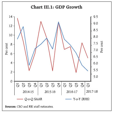
| Table III.1: Real GDP Growth | | (Per cent) | | Item | 2015-16 | 2016-17 | Weighted contribution to growth in 2016-17 (percentage points)* | 2015-16 | 2016-17 | 2017-18 | | Q1 | Q2 | Q3 | Q4 | Q1 | Q2 | Q3 | Q4 | Q1 | | Private Final Consumption Expenditure | 6.1 | 8.7 | 4.8 | 2.8 | 5.2 | 6.7 | 9.3 | 8.4 | 7.9 | 11.1 | 7.3 | 6.7 | | Government Final Consumption Expenditure | 3.3 | 20.8 | 2.0 | 0.9 | 4.3 | 4.2 | 4.1 | 16.6 | 16.5 | 21.0 | 31.9 | 17.2 | | Gross Fixed Capital Formation | 6.5 | 2.4 | 0.7 | 4.3 | 3.4 | 10.1 | 8.3 | 7.4 | 3.0 | 1.7 | -2.1 | 1.6 | | Net Exports | 15.1 | 37.4 | 0.4 | 1.6 | -5.3 | 27.4 | 95.3 | 36.6 | 59.3 | 30.8 | - | - | | Exports | -5.3 | 4.5 | 0.9 | -6.1 | -4.1 | -8.7 | -2.3 | 2.0 | 1.5 | 4.0 | 10.3 | 1.2 | | Imports | -5.9 | 2.3 | 0.5 | -5.9 | -3.4 | -9.9 | -4.3 | -0.5 | -3.8 | 2.1 | 11.9 | 13.4 | | GDP at Market Prices | 8.0 | 7.1 | 7.1 | 7.6 | 8.0 | 7.2 | 9.1 | 7.9 | 7.5 | 7.0 | 6.1 | 5.7 | *: Component-wise contributions to growth do not add up to GDP growth in the table because change in stocks, valuables and discrepancies are not included.
Source: Central Statistics Office (CSO). | III.1.1 Private Final Consumption Expenditure Even as PFCE remained the key driver of aggregate demand in the economy, contributing 54 per cent to real GDP, a marked deceleration has characterised its evolution in Q4:2016-17 and Q1:2017-18 in comparison with the preceding three quarters (Chart III.2). 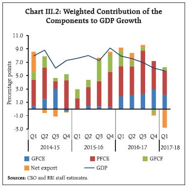 High frequency indicators for urban consumption paint a mixed picture, with sales of passenger cars and international air passenger traffic remaining robust, but consumer durables production having contracted (Chart III.3a). Going forward, urban consumption is expected to revive, following the upward revision in house rent allowances (HRA) for central government employees as also the likely implementation of the 7th Central Pay Commission (CPC) award at the sub-national level. High frequency indicators of rural demand, viz., growth in sales of two-wheelers and tractors, have witnessed sequential improvement in the recent months. The production of consumer non-durables, representing cash-intensive fast moving consumer goods (FMCG) demand, has, however, decelerated, though still exhibiting high growth among the components of industrial production (Chart III.3b). 
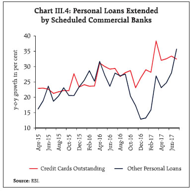 Retail consumption activity, reflected in drawals of personal loans from scheduled commercial banks (SCBs), suggests that underlying conditions are supportive of consumption demand, going forward (Chart III.4). III.1.2 Investment Demand Investment demand remained depressed, with its share in GDP declining from 34.3 per cent in 2011-12 to 29.5 per cent in 2016-17. Although GFCF exhibited a slender recovery in Q1:2017-18, the overall investment climate remains bleak. Subdued levels of investment activity were also reflected in the contraction of capital goods production, notwithstanding robust growth in imports of certain capital goods (III.5a). The corporate investment cycle is weighed down by excess capacity in the manufacturing sector. Capacity utilisation (CU) improved in Q4:2016-17, but it again dipped in Q1:2017-18, reflecting weak demand (Chart III.5b). High levels of stress in the balance sheets of banks and corporations continued to act as a drag on investment activity. Besides, households’ investment in dwellings, other buildings and structures also remained subdued due to high levels of inventories of residential houses and expectations of correction in prices. 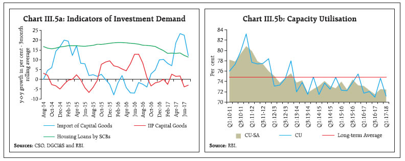 According to the Centre for Monitoring Indian Economy (CMIE), new investment proposals significantly declined in Q2: 2017-18 in terms of both numbers and value (Chart III.6a). Only 403 new projects were announced, the lowest since Q1:2004-05. The implementation of stalled projects still lacks adequate traction – there was a significant increase in stalled projects in Q1:2017-18; however, an improvement was reported in Q2:2017-18 (Chart III.6b). At the same time, anecdotal evidence suggests that awarding and construction of highway projects in the road sector have reached an all-time high and the daily additions of road construction have touched a peak. Some momentum in investment activity is also visible in sectors such as electricity transmission, roads and renewable power. Going forward, an increase in allocation of capital expenditure by 6.7 per cent in 2017-18 is expected to generate some multiplier and crowding-in effects, although a durable turnaround in the investment cycle largely hinges on a revival in private investment appetite. III.1.3 Government Expenditure As stated earlier, the slowdown in aggregate demand in Q1:2017-18 was cushioned by GFCE. Following advancement of the announcement of the Union Budget, the Centre undertook massive frontloading of expenditure. The disbursement of subsidies during April-August 2017, in particular, increased sharply. Consequently, revenue expenditure accounted for about 46 per cent of the budgeted expenditure (Table III.2). During Q2 so far (July-August 2017), revenue expenditure propped up GFCE with y-o-y growth of 4.4 per cent (-7.6 per cent in July-August 2016). | Table III.2: Key Fiscal Indicators – Central Government Finances (April-August) | | Indicator | Actual as per cent of BE | | 2016-17 | 2017-18 | | 1. Revenue Receipts | 28.0 | 27.0 | | a. Tax Revenue (Net) | 26.6 | 27.8 | | b. Non-Tax Revenue | 32.5 | 24.0 | | 2. Total Non-Debt Receipts | 12.7 | 18.4 | | 3. Revenue Expenditure | 41.0 | 45.8 | | 4. Capital Expenditure | 37.0 | 35.4 | | 5. Total Expenditure | 40.5 | 44.3 | | 6. Gross Fiscal Deficit | 76.4 | 96.1 | | 7. Revenue Deficit | 91.8 | 134.2 | | 8. Primary Deficit | 565.9 | 1401.3 | BE: Budget estimates.
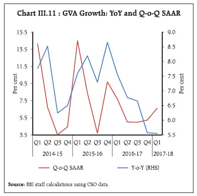
Source: Controller General of Accounts (CGA). | Tax revenues (net) were higher during April-August 2017 than their levels a year ago on account of higher collections under corporate and income taxes. Receipts under customs duties, union excise duties and service tax moderated, however, mainly due to the ongoing migration of select indirect taxes to the GST (Chart III.7a). Uncertainty on the revenue front can have adverse implications for the viability of government finances, going ahead. The GST Council recommended a four-tier rate structure – 5, 12, 18 and 28 per cent – for the fitment of all 1,211 items of goods and services, including exemptions on basic necessities (Chart III.7b). After the introduction of the GST, the total tax incidence on motor vehicles (GST plus Compensation Cess) has come down vis-a-vis the total tax incidence in the pre-GST regime. Accordingly, the GST Council has recommended that the central government moves legislative amendments for increasing the maximum ceiling of cess to be levied on motor vehicles to 25 per cent from 15 per cent. Meanwhile, the government has also indicated that it would further rationalise rates, depending on the progress of implementation. The number of new taxpayers who registered with the GSTN up to August 29, 2017 reached around 1.9 million. As per the latest information (up to September 25, 2017), revenue collections under GST for the month of August amounted to ₹906.7 billion as against ₹940.6 billion for the month of July, 2017.1 Going forward, the gains from expansion of the tax base due to introduction of the GST and improved tax compliance post-demonetisation are expected to improve tax buoyancy over the medium-term. 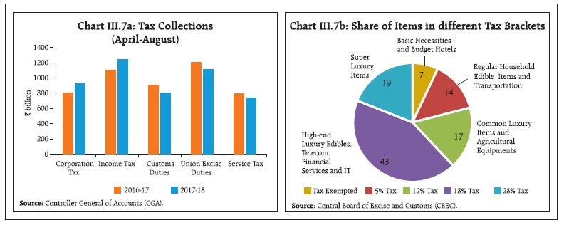 Nevertheless, businesses have been facing some IT challenges during the initial stage of implementation which are being looked into by the GST Council. After GST implementation, exporters can avail input tax credit only after sale within the domestic tariff area or after sending their shipments outside the country. They can subsequently claim the unutilised credit as refund, a process in which their working capital gets immobilised, thereby raising their operating cost. As exporters raised concerns over blockage of refunds and working capital on account of rollout of GST, the government has decided to refund substantial amount of taxes paid by them to provide immediate relief. In view of the difficulties being faced by taxpayers in filing returns, the dates for filing various GSTR have been extended. Furthermore, comprehending GST provisions and their impact on business along with the requirements for GST-compliance is still premature. Moreover, provisions for anti-profiteering as well as the now-deferred e-way bill which tracks consignments across states are unclear. After the fitment committee observed anomalies in GST levied on 40 items, the GST Council has lowered taxes on these products. In view of the above, it may be challenging to realise the projected tax revenues in the Union Budget 2017-18. The Centre’s borrowing programme was conducted as per the planned issuance schedule within the overall contour of its debt management strategy. Following the strategy of front loading of issuances, the central government completed 64.1 per cent (58.6 per cent in corresponding period of 2016-17) of its budgeted gross borrowings (₹5,800 billion) by September 2017 (Table III.3). The spate of increased borrowing by the state governments may, however, exert pressure on the finite pool of investible resources and crowd out private investment. | Table III.3: Government Market Borrowings | | (₹ billion) | | Item | 2015-16 | 2016- 17 | 2017- 18 (up to Sept 29) | | Centre | States | Total | Centre | States | Total | Centre | States | Total | | Net Borrowings | 4,406 | 2,594 | 7,000 | 4,082 | 3,426 | 7,508 | 2,493 | 1,598 | 4,091 | | Gross Borrowings | 5,850 | 2,946 | 8,796 | 5,820 | 3,820 | 9,640 | 3,720 | 1,779 | 5,499 | | Source: RBI. | Consolidated state finances are budgeted to improve in 2017-18 on account of a lower gross fiscal deficit- GDP ratio. While the capital expenditure-GDP ratio is budgeted to be lower in 2017-18 than in the previous year, capital outlay is projected to remain unchanged, which augurs well for the quality of expenditure. State finances, however, are likely to come under stress during 2017-18 from farm loan waivers announced during the year so far, which are estimated at around 0.5 per cent of GDP, and partial implementation of the seventh pay commission recommendations. This, in turn, has to be financed by additional market borrowings which push up interest rates, not just for the States but for the entire economy. A collateral damage could be that private borrowers are crowded out as the cost of borrowing rises. Even if the loan waiver is accommodated within budgetary provisions, it may force cutbacks in other heads of expenditure. Experience has shown that the most vulnerable category is capital expenditure. Illustratively, Uttar Pradesh, which presented its budget after the announcement of the loan waiver, has built in a decline in capital outlay and capital expenditure by 26.2 per cent and 30.4 per cent, respectively, during 2017-18. On the other hand, Maharashtra, which presented its budget before the announcement, projected a decline of around 4.2 per cent in capital expenditure. This, in turn, might entail deterioration in the quality of expenditure with attendant implications for productivity. III.1.4 External Demand With import growth far outpacing that of exports, the contribution of net external demand to GDP turned negative in Q1:2017-18, as in the preceding quarter. The slowdown in exports in Q1: 2017-18 was broad-based and encompassed oil and non-oil segments accounting for 74 per cent of the export basket. During July 2017, export growth slowed further despite a sharp increase in oil exports, but revived in August 2017 largely due to an increase in engineering goods, electronic goods and drugs and pharmaceuticals exports. Merchandise import growth accelerated in Q1:2017-18, taking the trade deficit to its highest level since Q2:2013-14, despite crude oil prices being half the level that prevailed in 2013-14 (Chart III.8a). In July-August too, the merchandise trade deficit expanded unrelentingly on the back of sustained import demand. Notwithstanding declining oil import volumes, gold imports grew strongly in Q1:2017-18 in anticipation of GST implementation. However, they moderated sequentially during June-August 2017 as stockpiling eased, while remaining high on a y-o-y basis (Chart III.8b). 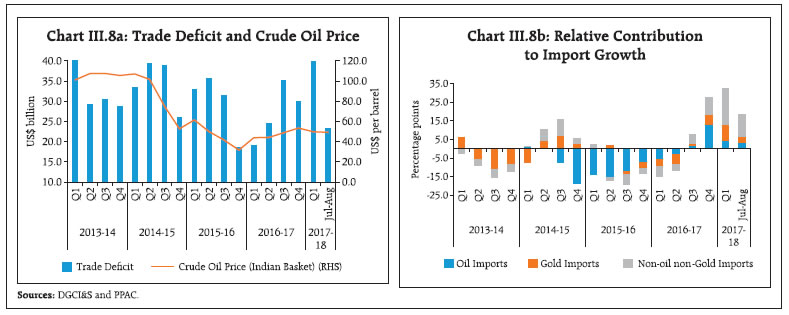 Among non-oil non-gold imports, which have been growing in double digits since Q4:2016-17, pearls and precious stones, electronics goods, coal and other goods contributed sizably, underlining the role of international commodity prices and increased domestic demand for electric, construction and dairy machinery even as a decline in imports of transport equipment coincided with an increase in domestic production (Chart III.9). While there has been a contraction in domestic production of capital goods, imports of capital goods, except transport equipment, gradually increased during April-August 2017. Similarly, higher imports of sugar reflected domestic consumption exceeding production in 2016-17. 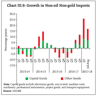 Net services receipts increased by 15.7 per cent on a y-o-y basis during Q1: 2017-18 largely driven by a rise in net earnings from travel, construction and other business services. While outflows of primary income remain a drag on the current account deficit (CAD), a modest rise in secondary income, primarily in the form of workers’ remittances, provided a partial offset. Both net FDI and net FPI flows to India rose during Q1:2017-18 over their levels a year ago, attesting to the attractiveness of the Indian economy as an investment destination. External commercial borrowings (ECBs) inflows also picked up modestly on the back of a sharp increase in issuance of rupee denominated bonds. In contrast, net accretion to NRI deposits declined marginally, reflecting lower inflows into Non-Resident External (NRE) rupee accounts. reflecting external sector resilience, foreign exchange reserves reached a level of US$ 399.7 billion on September 29, 2017 equivalent to 11.5 months of imports.2 III.2 Aggregate Supply The cyclical slowdown that set in at the beginning of 2016-17 pulled the growth of output measured by gross value added (GVA) at basic prices down to 5.6 per cent in Q1:2017-18, flat at the level of the preceding quarter (Table III.4). | Table III.4: Sector-wise Growth in GVA | | (Per cent) | | Sector | Weighted Contribution 2016-17 | 2015-16 | 2016-17 | 2015-16 | 2016-17 | 2017-18 | | Q1 | Q2 | Q3 | Q4 | Q1 | Q2 | Q3 | Q4 | Q1 | | Agriculture and Allied Activities | 0.8 | 0.7 | 4.9 | 2.4 | 2.3 | -2.1 | 1.5 | 2.5 | 4.1 | 6.9 | 5.2 | 2.3 | | Industry | 1.6 | 10.2 | 7.0 | 7.7 | 9.2 | 12.0 | 11.9 | 9.0 | 6.5 | 7.2 | 5.5 | 1.5 | | Mining and Quarrying | 0.1 | 10.5 | 1.8 | 8.3 | 12.2 | 11.7 | 10.5 | -0.9 | -1.3 | 1.9 | 6.4 | -0.7 | | Manufacturing | 1.4 | 10.8 | 7.9 | 8.2 | 9.3 | 13.2 | 12.7 | 10.7 | 7.7 | 8.2 | 5.3 | 1.2 | | Electricity, gas, water supply and other utilities | 0.2 | 5.0 | 7.2 | 2.8 | 5.7 | 4.0 | 7.6 | 10.3 | 5.1 | 7.4 | 6.1 | 7.0 | | Services | 4.3 | 9.1 | 6.9 | 8.9 | 9.0 | 9.0 | 9.4 | 8.2 | 7.4 | 6.4 | 5.7 | 7.8 | | Construction | 0.1 | 5.0 | 1.7 | 6.2 | 1.6 | 6.0 | 6.0 | 3.1 | 4.3 | 3.4 | -3.7 | 2.0 | | Trade, hotels, transport, communication | 1.5 | 10.5 | 7.8 | 10.3 | 8.3 | 10.1 | 12.8 | 8.9 | 7.7 | 8.3 | 6.5 | 11.1 | | Financial, real estate and professional services | 1.2 | 10.8 | 5.7 | 10.1 | 13.0 | 10.5 | 9.0 | 9.4 | 7.0 | 3.3 | 2.2 | 6.4 | | Public administration, defence and other services | 1.4 | 6.9 | 11.3 | 6.2 | 7.2 | 7.5 | 6.7 | 8.6 | 9.5 | 10.3 | 17.0 | 9.5 | | GVA at Basic Prices | 6.6 | 7.9 | 6.6 | 7.6 | 8.2 | 7.3 | 8.7 | 7.6 | 6.8 | 6.7 | 5.6 | 5.6 | | Source: Central Statistics Office (CSO). | Underlying this subdued performance was the depressed state of industrial activity, particularly manufacturing. Although agricultural and allied activities also decelerated sequentially from Q3:2016- 17, they were in alignment with the typical outturn in the first quarter of the year. Services sector activity, however, posted a strong performance, dispelling the slack that had manifested itself through 2016- 17. In fact, the deceleration of GVA was cushioned by continuing strong growth in public administration, defence and other services (PADO) growth, a constituent of the services sector which has been buoyed by frontloading of Government expenditure in Q1:2017-18. Excluding this component, the GVA growth would have slipped to 5 per cent in Q1:2017-18 (Chart III.10). However, seasonally adjusted q-o-q annualised GVA growth suggests a modest strengthening of momentum in Q1:2017-18 vis-à-vis Q4:2016-17 (Chart III.11). 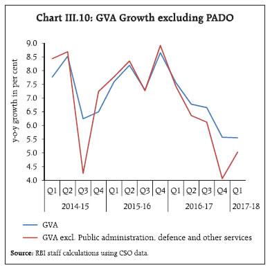
 The April MPR had projected GVA growth of 6.7 per cent for Q1:2017-18. The actual outcome undershot this projection by more than a full percentage point, indicative of the larger than expected loss of momentum (Chart III.12). The unexpected moderation in allied activities weighed heavily on the rate of growth of agricultural sector. In addition, the deceleration in the manufacturing sector reflected uncertainties surrounding GST implementation and higher than expected rise in input costs. III.2.1 Agriculture Agriculture and allied activities recorded a significant deceleration in Q1:2017-18 from Q4:2016-17, notwithstanding the jump of 8.5 per cent in rabi foodgrain production, the highest growth recorded in the last 13 years. Moreover, the area under horticulture grew by 2.6 per cent in 2016-17 from a year ago, while production increased by 4.8 per cent, reaching a record of 300 million tonnes. The moderation in agricultural GVA growth in relation to the preceding quarters mainly reflects the slowdown in ‘livestock products, forestry and fisheries’. South-west monsoon rainfall was higher than the long period average (LPA) till the fourth week of July, but turned significantly weak thereafter (Chart III.13). As of September 30, 2017, out of the 36 sub-divisions in the country, 30 divisions received excess/normal rainfall, while the remaining divisions (east and west UP, Haryana, Chandigarh & Delhi, Punjab, east MP and Vidarbha), covering 17 per cent of the sub-divisional area of the country, received deficient rainfall. In terms of the production weighted rainfall index (PRN), rainfall was lower than the previous year by 5 per cent, resulting in contraction in the area sown under key crops (Chart III.14). 
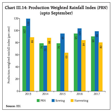 Although kharif sowing started on a high note, the momentum slowed down in August due to a lull in the south-west monsoon and lower than expected increase in MSPs (Table III.5) and decline in wholesale prices of major food items across mandis on account of the bumper harvest. The latest data suggest that sowing picked up again in September; however, kharif sowing for the year as a whole has remained lower than last year’s acreage (Chart III.15). In terms of crops, sown area was lower in the case of rice, coarse cereals, oilseeds pulses and jute and mesta, but it was higher in the case of sugarcane and cotton (Chart III.16). According to the first advance estimate (AE), the production of kharif foodgrains for 2017-18 at 134.7 million tonnes was 2.8 per cent lower than last year (4th AE). | Table III.5: Minimum Support Price (MSP) for Kharif Crops | | | MSP (Rs/Quintal) | y-o-y growth in per cent | | 2015-16 | 2016-17 | 2017-18 | 2016-17 | 2017-18 | | Paddy Common | 1410 | 1470 | 1550 | 4.3 | 5.4 | | Paddy (F)/Grade 'A' | 1450 | 1510 | 1590 | 4.1 | 5.3 | | Jowar-Hybrid | 1570 | 1625 | 1700 | 3.5 | 4.6 | | Jowar-Maldandi | 1590 | 1650 | 1725 | 3.8 | 4.5 | | Bajra | 1275 | 1330 | 1425 | 4.3 | 7.1 | | Ragi | 1650 | 1725 | 1900 | 4.5 | 10.1 | | Maize | 1325 | 1365 | 1425 | 3.0 | 4.4 | | Tur (Arhar) | 4625 | 5050 | 5450 | 9.2 | 7.9 | | Moong | 4850 | 5225 | 5575 | 7.7 | 6.7 | | Urad | 4625 | 5000 | 5400 | 8.1 | 8.0 | | Groundnut | 4030 | 4220 | 4450 | 4.7 | 5.5 | | Sunflower Seed | 3800 | 3950 | 4100 | 3.9 | 3.8 | | Soyabean Black | 2600 | 2775 | 3050 | 6.7 | 9.9 | | Soyabean Yellow | 2600 | 2775 | 3050 | 6.7 | 9.9 | | Sesamum | 4700 | 5000 | 5300 | 6.4 | 6.0 | | Nigerseed | 3650 | 3825 | 4050 | 4.8 | 5.9 | | Medium Staple Cotton | 3800 | 3860 | 4020 | 1.6 | 4.1 | | Long Staple Cotton | 4100 | 4160 | 4320 | 1.5 | 3.8 | | Source: Ministry of Agriculture and Farmers’ Welfare, Government of India. |
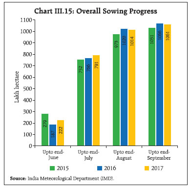
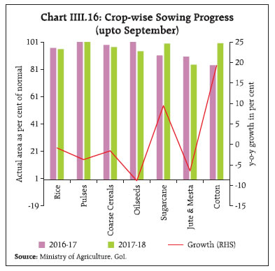 Water storage levels in 91 reservoirs across the country were lower at 66 per cent of the full reservoir level (74 per cent last year) as on September 28, 2017. Apart from the northern region, reservoirs in all other regions received less water than in the corresponding period last year. This could pose a challenge to the attainment of the crop production target set at 274.6 million tonnes for 2017-18. III.2.2 Industrial Sector Industrial GVA growth dipped to 1.5 per cent in Q1 of 2017-18 – the lowest in the last 20 quarters, mainly due to GST-related uncertainties. The index of industrial production (IIP) exhibited a broad-based deceleration in Q1. Large negative production effects partly offset positive base effects, especially in April and July (Chart III.17a). On a use-based analysis, the output of both capital goods and consumer durables contracted, highlighting weak investment appetite and slowing consumption demand. In terms of weighted contributions, the slowdown was led by capital goods, followed by intermediate goods (Chart III.17b). 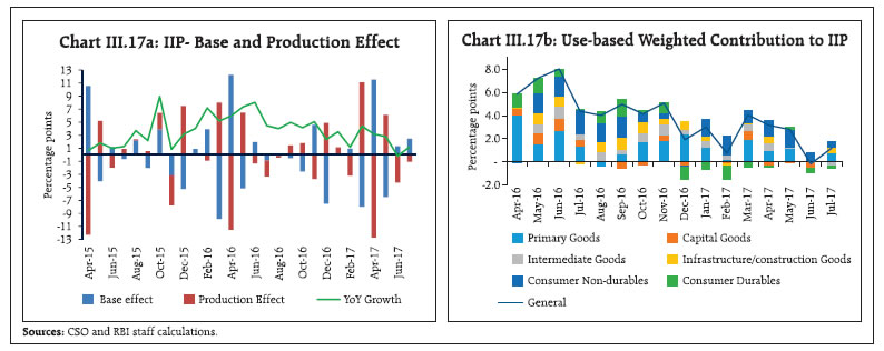
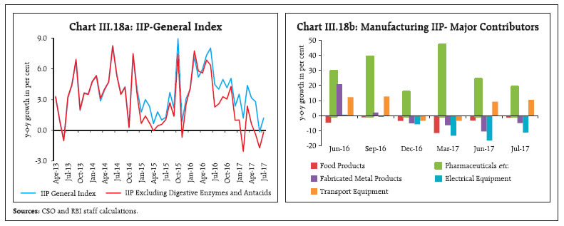 Acceleration in consumer non-durables was driven mainly by the contribution of a single item, viz., digestive enzymes and antacids (DEA); excluding this component, the overall index would have contracted by 0.2 per cent in July 2017 as compared with the growth of 2.2 per cent in July 2016 (Chart III.18a). Of the 23 industry groups that form the manufacturing sector, production in 15 industries contracted during July 2017. The strong performance in a few industries such as pharmaceuticals and transport equipment was pulled down by a broad-based slowdown in other industries, most notably electrical equipment (Chart III.18b). The sharp deceleration in manufacturing in Q1:2017- 18 was due to a combination of factors playing out simultaneously. While the uncertainties relating to GST implementation affected overall business sentiment, value added declined as sales decelerated and expenditure accelerated (Chart III.19). The mining and quarrying segment, which showed some signs of revival in the second half of 2016-17, sank back again to contraction mode in Q1:2017- 18. Although natural gas production has sustained the revival that set in from the second half of the previous year, contraction in crude oil production and subdued coal production pulled down mining output. Contraction in coal production was on account of lower demand for electricity generation, which has undergone significant transformation in the recent period. While renewable energy has made rapid strides due to falling costs and Government’s incentives, reports suggest that some of these projects are facing challenges in terms of collapse in prices resulting in low tariffs/renegotiations of tariffs, weak demand and exhausted tax benefits. These factors have raised concerns about the viability of such projects. Going forward, this segment may remain subdued until there is a significant pick-up in demand. The slowdown in IIP mirrored the lukewarm performance of eight core industries, except natural gas, coal and electricity. Contraction in cement, fertilisers and crude oil accentuated the overall slowdown. Early indicators for 2017-18 point to subdued industrial activity. The 79th round of the Reserve Bank’s Industrial Outlook Survey (IOS) signaled subdued demand conditions in Q2:2017-18.
III.2.3 Services The services sector, which decelerated sequentially through 2016-17, recorded a significant improvement in Q1:2017-18 (7.8 per cent, up from 5.7 per cent in Q4:2016-17), driven mainly by trade, hotels, transport and communication as well as public administration, defence and other services. Financial, real and professional services also showed improvement in Q1:2017-18. Although the construction sector switched from contraction mode in Q4:2016-17 into expansion, it may be too early to conclude that the upturn is durable (Chart III.20). In the housing sector, new units launched have slowed down although units sold have shown an uptick in some cities in recent quarters (Chart III.21a and b). This is expected to continue as the industry gears up for further consolidation, and as greater clarity on the implementation of Real Estate Regulatory Act (RERA) across States emerges. With large unsold inventories, property prices showed a correction in Q4:2016-17 in major cities (Chart III.22a). Cement production – an indicator of construction activity – is still in contraction mode, while steel consumption improved in recent months (Chart III.22b). Activity in trade, hotels, transport and communication, which was affected post-demonetisation, bounced back to register a five-quarter high growth of 11.1 per cent in Q1:2017-18. Indirect taxes, a major indicator of activity of this segment, grew by 14 per cent in Q1:2017-18. Most of the lead indicators of activity in this segment, viz., foreign tourist arrivals, international passenger and air freight traffic, railway traffic, and telephone subscribers showed an uptick in recent months. Financial, real estate and professional services also accelerated in Q1:2017-18, partly reflecting robust value addition by information technology companies in the professional services segment. The financial sector’s growth decelerated in the recent period, mirrored in weak growth in aggregate deposits and bank credit. Notwithstanding low credit growth, high deposit growth in the second half of 2016-17 had helped in propping up activity in this sub-sector, maintaining the weighted average of the two. In Q1:2017-18, however, both credit growth and deposit growth declined, pulling down the sub-sectoral activity (Chart III.23). As in the previous quarter, public administration, defence and other services benefitted from higher revenue expenditure of the Centre in Q1 and continued to provide support to GVA growth (Chart III.24). III.3 Output Gap The output gap measured by the deviation of actual output from its potential level and expressed as a percentage of potential output, is a gauge of demand conditions. Despite its usefulness as a summary measure of the cyclical component of aggregate demand, infirmities arise from the fact that the output gap is unobservable and needs to be estimated from the data. As different filtering techniques are highly sensitive to the choice of period, methodology and the availability of data, a pragmatic approach is followed by staff that involves various methodologies including univariate filters like Baxter-King (BK), Hodrick–Prescott (HP) and Christiano- Fitzgerald (CF), Multivariate Kalman filters (MVKF) and production functions. A finance adjusted measure of the output gap, which controls for the imbalances emanating from the financial sector, has also been introduced in this MPR (Box III.1). All these output gap measures are aggregated by using principal component analysis in order to construct a composite measure (Chart III.25 a and b). This measure indicates that the output gap has been negative since Q3:2016-17. 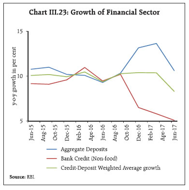
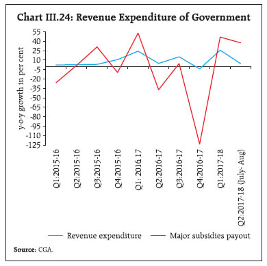 Box III.1: Finance Neutral Output Gap The estimation of potential output - the level of output that an economy can produce sustainably over the medium-term consistent with low and stable inflation – enables an assessment of the output gap as the deviation of actual output from this potential level. Conventional estimates of the output gap largely ignore the role of financial sector (Borio et al., 2016). The preglobal financial crisis (GFC) period was characterised by high output growth, benign inflation and financial sector imbalances emanating from rapid growth in credit and asset prices, which eventually culminated in the GFC in 2008. It is plausible for inflation to remain low and stable in times when output growth is on an unsustainable path due to buildup of imbalances in financial sector. Taking these into consideration Borio et al. (2016) present an alternate measure of the output gap – “finance neutral output gap” – which incorporates the role of financial sector variables in the evolution of economic cycles. India also recorded high credit and asset prices growth along with rising output growth and moderately low inflation in the pre-GFC period. For instance, during 2002-03 to 2007-08 the average annual growth in nonfood credit and annual return on assets (measured by the Sensex) were 27 per cent and 32 per cent, respectively, while the CPI inflation was, on an average, about 5 per cent. Output growth was close to double digits during 2005-06 to 2007-08 (Chart a). Guided by empirical evidence of a significant relationship between financial factors and business cycles, real credit growth and real asset price growth were included along with the real policy rate to estimate the output gap in a semi-structural multivariate Kalman filter framework. The finance neutral output gap was estimated using quarterly data from Q1:2006-07 to Q1:2017-18 by the quasi maximum likelihood method on the following state space model:
The historical decomposition of the output gap, portraying the contribution of various factors on its evolution, suggests that financial factors have been contributing negatively to the output gap since 2012-13 (Rath et.al, 2017) (Chart c). High inflation and low real interest rates during the period 2010-13 contributed positively to the output gap. More recently, subdued credit growth has contributed negatively to demand conditions. References: Borio, C., Disyatat, P., & Juselius, M. (2016), “Rethinking Potential Output: Embedding Information about the Financial Cycle’’, Oxford Economic Papers, 69(3), 655- 677. Rath, D.P., Mitra, P. and John, J. (2017), “A Measure of Finance-Neutral Output Gap for India”, RBI Working Paper Series, WPS (DEPR): 03 / 2017. Conclusion Early indicators for Q2:2017-18 point to subdued industrial activity, in particular in the manufacturing sector. While many high frequency services sector indicators show signs of improvement, some others such as port traffic and domestic air freight traffic still show tepid growth. The Government’s initiatives in essential infrastructure, affordable housing, improved customer protection and transparency through the real estate regulatory act should be positive for construction activity, if they are implemented with speed and efficiency. The GST is likely to result in greater formalisation of the economy in due course as firms register to receive input tax credits even though teething problems remain a challenge at the current juncture. Improved prospects for rural incomes during 2017-18, higher MSPs, and large budgetary allocations for MGNREGA could lead to improvement in rural demand. Household consumption demand in urban areas may get a boost from the upward revision in HRA for government employees and implementation of the 7th CPC announced by States. The key to achieving a higher growth trajectory lies, however, in reviving investment activity. Major structural reforms already initiated, including the GST, enactment of the Insolvency and Bankruptcy Code (IBC), the likely recapitalisation of public sector banks and speedy resolution of stressed assets augur well for the outlook. 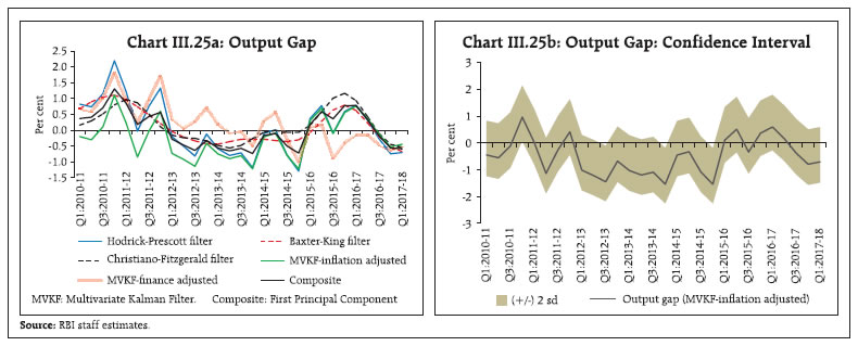
|
IV. Financial Markets and Liquidity Conditions Financial market conditions in the first half of 2017-18 remained stable, with the weighted average call money rate (WACR) moving progressively closer to the policy repo rate, stock markets scaling new highs, bond yields oscillating with fluctuations in inflation readings and the foreign exchange market buoyed by large portfolio flows. Credit offtake from risk-averse banks remained low, though monetary policy transmission strengthened for new loans in conditions of sizable surplus liquidity. Through the first half of 2017-18, global financial markets were lifted by record low volatility, declining credit spreads and stretched market valuations, as concerns about the pace of reflation and normalisation of monetary policy in advanced economies (AEs) receded. Equity markets scaled new peaks relative to earnings, propelled by a renewed reach for returns. Bond yields, which had firmed up till early 2017, reversed course from April on softer than expected commodity prices and expectations of a more relaxed pace of monetary policy normalisation in the US on easing inflation risks. The US dollar depreciated against major currencies, partly correcting for the upside it had gained post-Presidential elections in the US. Geopolitical risks, however, sparked bouts of volatility in August. Global financial markets remained largely resilient to the September communication of the Federal Reserve on its balance sheet normalisation. Financial markets in emerging market economies (EMEs) remained tranquil, with equity markets surging and the return of large portfolio flows exerting appreciation pressures on their currencies. Domestic financial markets were influenced by a variety of factors: the dramatic swings in inflation; surplus liquidity conditions; the implementation of GST; and remonetisation. The weighted average call money rate (WACR) – the operating target of monetary policy – moved closer to the policy repo rate, notwithstanding persistent surplus liquidity conditions. Equity markets were buoyed to new peaks by a surge in investment by mutual funds, even as foreign portfolio investment reached close to exhausting macro-prudential limits in some debt markets. Corporate bond yields softened, tracking G-sec yields and moderation in credit spreads. The exchange rate of the rupee moved in a narrow range, with an appreciating bias on the back of waves of portfolio flows. Markets were impacted in September by the announcement of the Fed that it will initiate balance sheet normalisation in October and certain domestic developments, in particular, higher inflation print and concerns about the rise in the fiscal deficit, leading to hardening of yields, correction in stock prices and depreciation of the rupee. Deposit rates declined as banks were flush with liquidity. Credit flows from banks improved modestly, though still hamstrung by stressed assets induced deleveraging and weak investment demand. A cumulative 200 basis points (bps) cut in the repo rate since January 2015 has been, by and large, transmitted to lending rates on new loans; however, transmission to past loans remains incomplete. IV.1 Financial Markets Different market segments in the domestic financial system responded variedly to domestic cues, with the impact of global spillovers remaining relatively contained until mid-September. Excess liquidity in money markets, high valuations in the bond and equity markets and an upside tone in the forex market co-existed with subdued activity in the credit market in the first half of 2017-18. IV.1.1 Money Market: A large liquidity overhang, fuelled mainly by the front-loading of government spend, which necessitated frequent recourse to ways and means advances (WMAs) and overdrafts (ODs) over the greater part of this period, imparted a downside bias to overnight money market rates in H1 of 2017-18. While the liquidity adjustment facility (LAF) corridor was narrowed from +/- 50 bps to +/- 25 bps in April 2017, active liquidity operations (described in Section IV.3) progressively whittled away at the overhang and narrowed the spread between the WACR and the policy rate from 31 bps in April to 13 bps in September (Charts IV.1 and IV.2). In combination with the liquidity impact of the RBI’s forex operations and scheduled redemptions of G-secs, these autonomous flows more than offset the liquidity tightening impact of remonetisation. 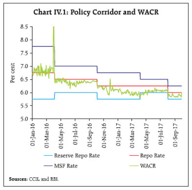 Money market rates adjusted seamlessly to the narrowing of the LAF corridor. Virtually no effect was observed on volumes traded in the call money market (Charts IV.3 and IV.4). Empirical evidence suggests that volatility in the WACR has a relatively muted role in monetary policy transmission (Box IV.1). 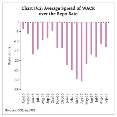 Other money market rates traded in alignment with the WACR (Chart IV.5). In view of comfortable access to liquidity and weak demand for credit, banks reduced their recourse to certificates of deposit (CDs). Fresh issuances of CDs were lower at ₹1,302 billion during H1 of 2017-18 (up to September 1, 2017) as against ₹1,518 billion during the corresponding period of 2016-17. With the lower-than-expected CPI inflation reading in May 2017, money market rates traded with an easing bias, especially in the secondary segments. Since May 12, 2017, 3-month commercial paper (CP), 3-month CDs and 91-day Treasury Bill (T-Bill) rates declined by 15 bps, 20 bps and 20 bps, respectively. After the repo rate was cut in August 2017, the 3-month CD and 91-day T-Bill rates declined by about 10 bps and 5 bps, respectively, while the 3-month CP rate inched up by about 4 bps, indicating that markets had already priced in a repo rate cut. 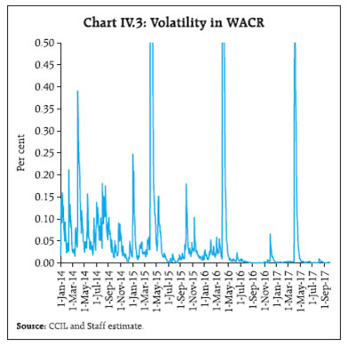
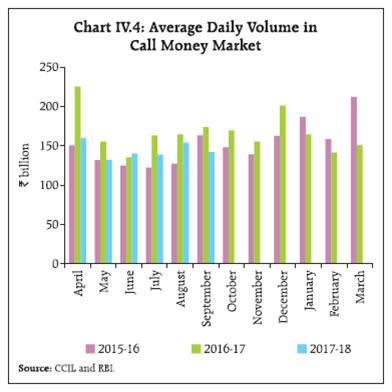 Box IV.1: Operating Target Volatility and Monetary Policy Transmission High volatility in the operating target can potentially dampen transmission of monetary policy. Changes in long-term interest rates, which are vital to monetary policy transmission for influencing aggregate demand, are conditioned by the expected path of future short-term rates and variations in the term premium. Higher volatility in overnight rates can potentially spillover into the term premium, thereby influencing “equilibrium levels of nominal and real long-term rates and disturbing the transmission mechanism of monetary policy impulses” (Colarossi and Zaghini, 2009). In the empirical literature, the transmission of volatility from the overnight interest rate along the yield curve is typically validated by the statistical significance of conditional volatility relating the overnight rate in variants of generalised autoregressive conditional heteroscedasticity (GARCH) specifications. Country experiences yield scant evidence of transmission of volatility from the overnight rate. Pro-active liquidity management and greater transparency along with more effective communication may help in better anchoring of market expectations (Osborne, 2016). With a view to studying the impact of conditional volatility of the WACR – the operating target of monetary policy in India – on interest rates across the term structure, the following GARCH (1,1) mean and volatility equations were specified.
| Table IV.B.1: Conditional Volatility of WACR using GARCH (1,1)* | | Dependent Variable: ∆WACR | | | Co-efficient | p-value | | Co-efficient | p-value | | Mean Equation | Volatility Equation | | Constant | -0.001 | 0.19 | RESID(-1)^2 | 0.244 | 0.00 | | Σ∆WACR | -0.24 | 0.00 | GARCH(-1)^2 | 0.756 | 0.00 | | Σ∆Repo Rate | 0.8 | 0.03 | Dum_March | 0.342 | 0.00 | | Net Liquidity | 0.002 | 0.00 | | | | | ECM | -0.050 | 0.00 | | | | | Dum_March | 1.186 | 0.00 | | | | | Dum_April | -1.413 | 0.00 | | | | | Dum_Taper | 0.136 | 0.00 | | | | | D3 | 0.039 | 0.00 | | | | | D10 | 0.004 | 0.09 | | | | | D11 | -0.010 | 0.00 | | | | | D13 | -0.004 | 0.04 | | | | | T-DIST. DOF | 3.244 | 0.000 | | | | | Q(10) | 12.446 | 0.256 | | | | | Q(20) | 23.144 | 0.282 | | | | | ARCH LM (5) | 0.430 | 0.828 | | | | *: Using dalily data since January 2009.
Source: RBI staff estimates. | Conditional volatility of the WACR extracted from equations (1) and (2) is then used as an explicit determinant of daily change in other interest rates (i.e., nominal yield on government paper of 3-month, 6-month, 9-month, 12-month, 2-year and 10-year maturities), in their respective mean and volatility equations, while retaining the same structural specifications as in equations 1 and 2. The coefficients of conditional volatility of WACR in the mean and variance equations of other interest rates are reported in Table IV.B.2. Two inferences could be derived from these results: (a) WACR volatility is not a statistically significant determinant of the mean values of daily changes in other interest rates across the yield curve; and (b) even while WACR volatility has a statistically significant conditioning influence on the volatility of other interest rates, particularly up to one year tenor, the values of the relevant coefficients are too small to impact the transmission of monetary policy. A one percentage point increase in volatility of the WACR is estimated to increase the volatility of short-term yields by about 0.02 to 0.08 bps, while the impact on volatility of longer-term yields is even more negligible. These findings suggest that occasional surges in volatility triggered by specific developments are likely anticipated and contained quickly through proactive liquidity management, which helps avert any potential impediments to the transmission of monetary policy. | Table IV.B.2: Impact of WACR Volatility Across the Term-structure of Interest Rates* | | (coefficients) | | | 3-month TB | 6-month TB | 9-month TB | 12-month TB | 2-year G-sec | 10-year G-sec | | Mean equation | -0.0059 | -0.0019 | -0.0042 | -0.0044 | -0.0001 | -0.0003 | | | (0.31) | (0.65) | (0.35) | (0.42) | (0.52) | (0.94) | | Variance equation | 0.0004 | 0.0002 | 0.0003 | 0.0008 | 0.0000 | 0.0001 | | | (0.00) | (0.00) | (0.00) | (0.00) | (0.04) | (0.00) | *: Using daily data since January 2009.
Note: Figures in parentheses indicate the p-values.
Source: RBI staff estimates. | References: Matthew Osborne (2016), “Monetary Policy and Volatility in the Sterling Money Market”, Bank of England Staff Working paper No. 588, April. Silvio Colarossi, and Andrea Zaghini (2009), “Gradualism, Transparency and the Improved Operational Framework: A Look at Overnight Volatility Transmission”, International Finance, Volume 12, Issue 2, Summer, Pages 151–170. | IV.1.2 Government Securities (G-sec) Market: G-sec yields generally softened during the most part of H1 of 2017-18, driven by lower inflation data, sustained demand from foreign portfolio investors, and the 25 bps cut in the repo rate by the Monetary Policy Committee (MPC) in August 2017. However, G-sec yields hardened thereafter reacting to the higher-than-expected August inflation print and the Fed communication on September 20, 2017 signalling one more possible rate hike in 2017 and the initiation of balance sheet normalisation from October 2017 (Chart IV.6). Market concerns about the likely increase in the domestic fiscal deficit due to a possible fiscal stimulus to boost the economy also impacted yields. 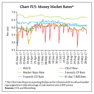
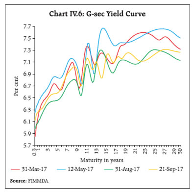 G-sec yields hardened by 12 bps in early April in anticipation of oversupply of paper because of the likely use of market stabilisation scheme (MSS) and open market operations (OMOs) by the RBI to absorb surplus liquidity. Two developments in the month of May, however, contributed to considerable softening of yields (Chart IV.7). First, a new benchmark Government of India Security of 10-year tenor (NI GS 2027) was auctioned on May 12, 2017 at a cut-off of 6.79 per cent, evincing an enthusiastic bid-cover ratio of 6.61. Second, the CSO’s May 12 release on CPI – coinciding with the date of auction of the new benchmark – showed headline inflation softening in April 2017. In June, yields softened even further in response to headline inflation for May 2017 printing lower. In Q2, CPI inflation’s historic low reading for June 2017 at 1.5 per cent combined with the normal progress of the monsoon further boosted sentiment in the G-sec market. With the July CPI inflation moving up, however, expectations reversed and yields commenced hardening in August, notwithstanding the 25 bps cut in the repo rate. Notably, the normalisation of the US monetary policy during H1 of 2017 (on March 15 and on June 14) did not have much influence on domestic yields. However, G-sec yields hardened thereafter on the faster-than-expected rise in August headline inflation, the prospect of a fiscal stimulus in India, and the Fed communication of September 20, 2017, as mentioned earlier. 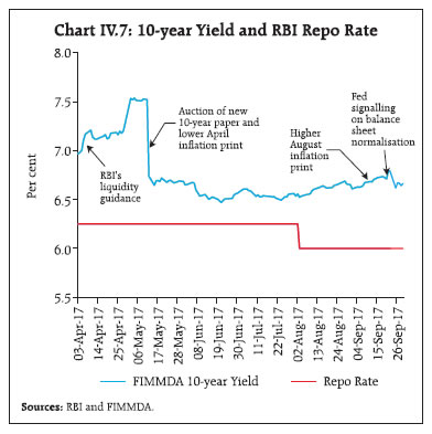 Persisting positive yield differentials with the rest of the world and the stable exchange rate of the rupee created congenial conditions for foreign portfolio inflows. Net foreign portfolio investment in G-secs was ₹617 billion (including investment in state development loans of ₹26.2 billion) during H1, resulting in 99 per cent of the limit for FPI investment in G-secs being utilised1. FPIs continued to be net buyers in the debt market in every month during H1 (Chart IV.8). In the short end of the G-sec market, the impact of the larger supply of paper – issuances of T-Bills of ₹1 trillion under the MSS and of cash management bills (CMBs) cumulatively aggregating to ₹2.5 trillion – was reflected in the hardening of T-Bills rates during H1 (Chart IV.9). Issuances of state development loans (SDLs) remained subdued in Q1 of 2017-18, but picked up in Q2. The spread of SDLs’ cut-off over the 10-year G-sec remained in the range of 74-87 bps in September 2017 as compared with 77-81 bps in April 2017 (Chart IV.10). In H1 of 2017-18, there were no issuances of Ujwal DISCOM Assurance Yojana (UDAY) bonds in contrast to 2016-17 when thirteen States issued UDAY bonds of ₹1,091 billion as against ₹990 billion issued by eight States in the previous year2. The total secondary market trading volume (face value) of UDAY bonds during H1 of 2017-18 (up to September 29, 2017) was ₹626 billion. 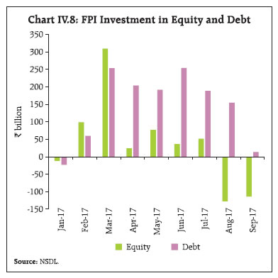
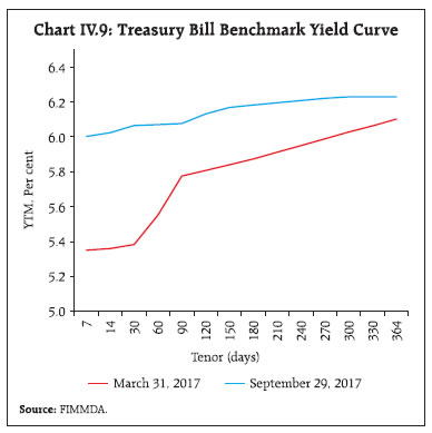
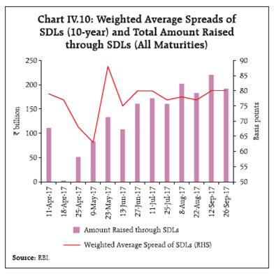 There is no significant relationship between the borrowing spreads on SDLs and States’ fiscal deficits and debt positions. The inter-State spread was, on average, within 9 bps during H1 of 2017-18 as against 7 bps in 2016-17 and 2015-16. Cost considerations have drastically reduced the dependence of State Governments on the National Small Savings Fund (NSSF). Following the recommendations of the 14th Finance Commission (FC), all States (barring four3) have been allowed to be excluded from the NSSF financing facility beginning 2016-17. The share of market borrowings, which can be raised at relatively lower costs, particularly when markets do not differentiate between States on the basis of their respective fiscal deficits and debt, has increased, including for discharging past NSSF liabilities. IV.1.3 Corporate Bond Market: Corporate bond yields softened during H1 of 2017-18, tracking the decline in G-sec yields (Chart IV.11a). The decline in 5-year AAA corporate yield was, however, interspersed with occasional spikes at the end of June and in early-July. The spread of 5-year AAA rated corporate bonds over 5-year G-secs declined by 56 bps, possibly reflecting improvement in overall credit risk perceptions on expectation of faster resolution of stressed assets under the Banking Regulation (Amendment) Ordinance promulgated on May 4, 2017. The average daily turnover in the corporate bond market increased sharply to ₹73.2 billion during April-August 2017 from ₹47.5 billion during the corresponding period of last year. Resources mobilised through issuances of corporate bonds in the primary market increased by 7.1 per cent to ₹2,770 billion during April-August 2017 from ₹2,588 billion a year ago. Of the total resources mobilised from the private corporate bond market, private placements constituted 98.6 per cent (Chart IV.11b). Foreign portfolio investment (FPI) in corporate bonds increased to ₹2.42 trillion as on September 28, 2017 from ₹1.86 trillion at end-March 2017. As a result, the utilisation of the approved limit rose to 99.2 per cent from about 76 per cent at end-March 2017. On September 22, 2017, the Reserve Bank announced the removal of Masala bonds or rupee denominated bonds issued overseas from the corporate bond investment limit effective October 3, 2017. This will release additional space for investment by FPIs in corporate bonds. The total investment in Masala bonds amounted to ₹440 billion at end-September 2017. The stable exchange rate of the rupee, uncertainty around policies of the US administration, and market expectations of a more gradual Fed normalisation increased the attractiveness of Indian bonds. 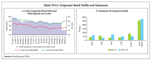 IV.1.4 Stock Market: The equity market remained buoyant through the greater part of H1 of 2017-18, with the BSE Sensex crossing the 32,000 mark on July 13, 2017 and the NSE Nifty crossing the 10,000 mark on July 26, 2017. Upbeat market sentiment appeared impervious to the perception of overvaluation in terms of a high price to earnings ratio (about 23.4) at end-September 2017 relative to AEs (21.0) and EMEs (15.8). Market ebullience was largely generated by domestic factors: expectations of reform intensification after introduction of the GST; the resolution of bank stressed assets and smooth progress of the insolvency regime; satisfactory monsoon; and lower inflation in May and June. The BSE Sensex gained 5.6 per cent during H1 of 2017-18 (Chart IV.12a). Net buying by domestic institutional investors, particularly by mutual funds, overwhelmed volatile foreign portfolio flows and sustained the rally (Chart IV.12b). After a late April recovery from downside global cues and sporadic volatility in June, stock markets surged in July 2017, with both the BSE Sensex and the NSE Nifty touching historic highs. In August 2017, markets corrected somewhat amidst volatility following the SEBI’s directions to stock exchanges to ban shell companies, concerns over high valuations, lower than expected corporate earnings results for Q1 of 2017-18, downside risks to growth in 2017-18, uncertainty over the GST rollout, net selling by foreign portfolio investors and global sell-offs over geopolitical tensions in the Korean peninsula. 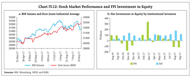 Reduction in deposit interest rates by banks and the decline in gold prices enhanced the relative attractiveness of mutual fund schemes. Resources mobilised under equity oriented schemes during April-August 2017 were higher at ₹614 billion than ₹185 billion during the corresponding period last year. Mutual funds are emerging as a counterweight to foreign institutional investors in the equity market. Net investment by mutual funds in equity during April-September 2017 was at ₹752.7 billion as against outflows of ₹87.7 billion by foreign portfolio investors. The post-demonetisation shift in the composition of financial saving of households into financial assets expanded assets under management (AUM) of mutual funds sizably from about ₹17.5 trillion at end-March 2017 to a record of ₹20.6 trillion at end-August 2017 as against assets under custody of FPIs of ₹30.4 trillion. In the primary market, resources mobilised through public issues of equity (initial public offers and rights issues) increased by 9.0 per cent during April-August 2017 over the corresponding period a year ago. Companies mobilised a total of ₹104.7 billion through 53 initial public offer (IPO) issues of which 41 were listed on the Small and Medium Enterprise (SME) platform of the BSE and the NSE. Financial entities accounted for 32.8 per cent of the total resources mobilised through public issues of equity. Among non-financial entities, the healthcare sector raised the largest amount of ₹19.5 billion, accounting for 26.1 per cent of the total, followed by engineering (20.1 per cent) and consumer service (10.6 per cent) sectors. The IPOs in the pipeline suggest that the upbeat primary market conditions are likely to continue in the short run. IV.1.5 Foreign Exchange Market: The rupee traded with an appreciating bias against the US dollar, strengthening by around 4 per cent in H1 of 2017-18 after six consecutive years of depreciation. A weaker US dollar and strong inflows drawn in by the resilience of macro fundamentals, especially the narrowing of inflation differentials, also provided sustained upside to the rupee, as in the case of the EME currencies (Chart IV.13). Expectations of bolder reforms after the State election results, the narrowing of the current account deficit in 2016-17 – in its July 2017 External Sector Report, the IMF assessed India’s external positions as “broadly in line” with medium-term fundamentals – and the implementation of the GST combined to lend an upside bias to the rupee. Notably, exchange rate volatility declined considerably: the coefficient of variation4 of the INR/USD exchange rate at 0.6 per cent during the first half of 2017-18 was lowest since 2005-06. 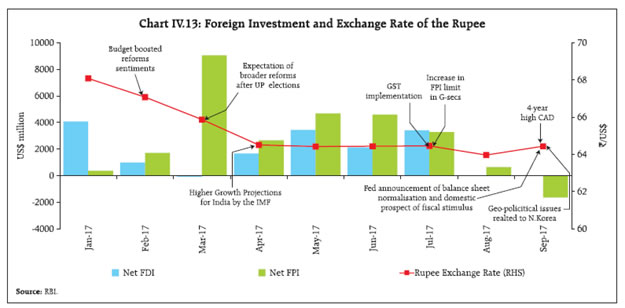
| Table IV.1: Nominal and Real Effective Exchange Rates: Trade-based (Base: 2004-05=100) | | Item | Index: September 29, 2017 (P) | Appreciation (+) / Depreciation (-) (Per cent) | | September 2017 over March 2017 | March 2017 over March 2016 | | 36-currency REER | 116.0 | -0.6 | 6.3 | | 36-currency NEER | 76.1 | -0.7 | 4.8 | | 6-currency REER | 130.3 | 0.1 | 8.0 | | 6-currency NEER | 67.2 | -2.7 | 5.5 | | ₹/ US$ (As on September 29, 2017) | 65.4 | 2.2 | 1.7 | P: Provisional.
Note: REER figures are based on the Consumer Price Index (Combined).
Source: RBI. | In terms of both the 36-currency nominal effective exchange rate (NEER) and the real effective exchange rate (REER), the rupee depreciated by 0.7 per cent and 0.6 per cent, respectively, between September 2017 and March 2017 (Table IV.1). Currencies of several major AEs and EMEs have appreciated against the US dollar since January 2017, largely reflecting the weakness of the US dollar, with the US dollar index depreciating by 8.9 per cent over end-December 2016 (Chart IV.14). IV.1.6 Credit Market: In the credit market, activity remained subdued although non-food credit staged a modest recovery during H1 of 2017-18, after a sharp deceleration in the preceding six months (Chart IV.15). A part of the credit slowdown in H2 of 2016-17 was overstated by the swapping of loans into UDAY bonds and the use of demonetised currency notes for repaying bank loans. As stated in the MPR of April 2017, stressed assets – gross NPAs of scheduled commercial banks (SCBs) at 10.3 per cent of total advances and the stressed advances ratio at 12.6 per cent as on June 30, 2017 – and capital constraints, particularly in public sector banks, have hindered a robust revival in the flow of bank credit. The large divergence in credit growth across bank groups is striking, suggesting the role of several factors at play from both demand side and supply side (Chart IV.16). 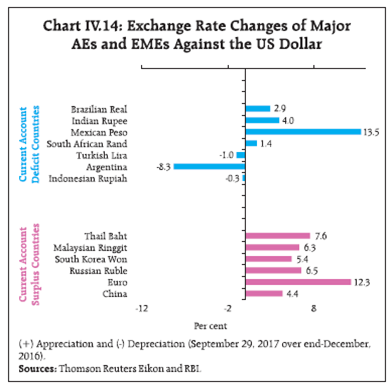 The adverse impact of stressed assets in the banking system is also visible in the sectoral deployment of credit (Chart IV.17). Industry has the largest share of stressed assets in the banking system and, correspondingly, credit growth to industry remains in contraction mode. Within industry, sectors facing acute stress are also experiencing the largest declines in bank credit exposure, reflecting stepped-up efforts to deleverage and free up balance sheets from impairment (Chart IV.18).
Banks also extend finance to the commercial sector of the economy by way of non-SLR investments, mainly in the form of investment in CPs and bonds/shares/debentures issued by non-financial corporates. In H1 of 2017-18, however, banks’ non-SLR investment was lower than in previous years (Chart IV.19). 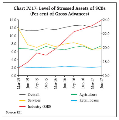 With the gradual reduction in surplus liquidity in the system and the pick-up in credit growth, the level of excess maintenance under the Statutory Liquidity Ratio (SLR) by the banking system declined from a high of 11.8 per cent in December 2016 to 9.2 per cent by June 2017 (Chart IV.20). The prescribed SLR was reduced by 50 bps to 20.0 per cent of NDTL effective the fortnight beginning June 24, 2017, aimed at freeing up resources of banks for lending to productive sectors of the economy. After the reduction in the SLR, however, excess SLR increased in July to 9.8 per cent and further to 10.3 per cent in August, reflecting banks’ reluctance to lend in the face of their asset quality concerns and capital constraints, lacklustre investment demand and stalled progress in unlocking stranded investment. The increase in excess SLR occurred across bank groups, but was the sharpest for foreign banks. Private banks, which have the lowest excess SLR among SCBs, also registered a sharp increase in August to 5.9 per cent of NDTL. High excess SLR has enabled banks to comfortably meet the liquidity coverage ratio (LCR) norms, relative to their counterparts in other jurisdictions. 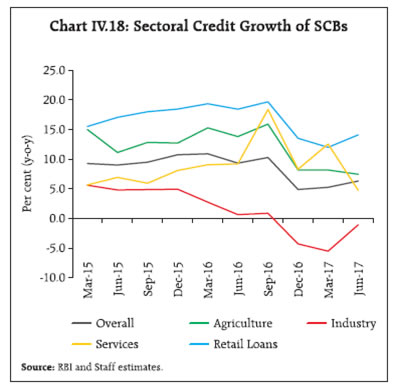
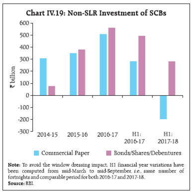
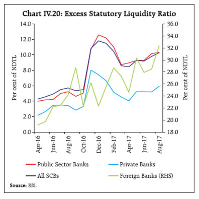 The total flow of financial resources to the commercial sector was much higher during H1 of 2017-18 than in the comparable period of last year5, with both bank and non-bank funding being higher (Chart IV.21). Among non-bank sources of funding, the increase was mainly on account of foreign sources, particularly FDI. Among domestic non-bank sources, credit extended by housing finance companies and NBFCs increased (Table IV.2). 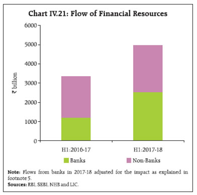
| Table IV.2: Funding from Non-Bank Sources to Commercial Sector | | (Amount in ₹ billion) | | Item | April to August | | 2016-17 | 2017-18 | | Amount | Per cent of total | Amount | Per cent of total | | A. Flow from Non-banks (A1+A2) | 2,266 | 100.0 | 2,575 | 100.0 | | A1. Domestic Sources | 1,802 | 79.6 | 1,616 | 62.8 | | 1 Public issues by non-financial entities | 60 | 2.6 | 80 | 3.1 | | 2 Gross private placement by non-financial entities | 615 | 27.2 | 449 | 17.4 | | 3 Net issuance of CPs subscribed by non-banks # | 720 | 31.8 | 148 | 5.7 | | 4 Net credit by housing finance companies $ | 332 | 14.7 | 510 | 19.8 | | 5 Total accommodation by 4 RBI regulated AIFIs | 4 | 0.2 | -5 | -0.2 | | 6 NBFCs-ND-SI (net of bank credit) # | 35 | 1.5 | 285 | 11.1 | | 7 LIC’s net investment in corporate debt, infrastructure and social sector | 36 | 1.6 | 148 | 5.8 | | A2. Foreign Sources | 463 | 20.4 | 959 | 37.2 | | 1 External commercial borrowings / FCCB $ | -204 | -9.0 | 47 | 1.8 | | 2 Foreign direct investment to India $ | 667 | 29.4 | 912 | 35.4 | #: Up to June 2017 $: Up to July 2017.
Sources: RBI, SEBI, NHB and LIC. |
| Table IV.3: Transmission to Deposit and Lending Rates | | (Variation in percentage points) | | Period | Repo Rate | Term Deposit Rates | Lending Rates | | Median Term Deposit Rate | WADTDR | Median Base Rate | WALR - Outstanding Rupee Loans | WALR - Fresh Rupee Loans | 1-year Median MCLR | | Sep. 15, 2017 over Dec. 2014 | -2.00 | -1.58 | -1.95 | -0.75 | -1.25 | -1.93 | -1.10 | | Pre-Demonetisation (Dec. 2014 to Oct. 2016) | -1.75 | -0.99 | -1.26 | -0.61 | -0.75 | -0.97 | -0.15 | | Post-Demonetisation (since Nov. 2016) | -0.25 | -0.59 | -0.69 | -0.14 | -0.50 | -0.96 | -0.95 | WADTDR: Weighted Average Domestic Term Deposit Rate. WALR: Weighted Average Lending Rate. MCLR: Marginal Cost of Funds Based Lending Rate. MCLR was introduced on April 1, 2016. Data on Median Term Deposit Rate, WADTDR and WALR on outstanding and fresh rupee loans pertain to August 2017. 1-year Median MCLR data relate to September 15, 2017.
Source: RBI. | IV.2 Monetary Policy Transmission The massive influx of current account and savings account (CASA) deposits into the banking system post-demonetisation brought about an appreciable reduction in the cost of funds of banks and helped strengthen the transmission of monetary policy to lending rates. While transmission was relatively stronger to deposit rates before demonetisation, the transmission to marginal cost of funds based lending rate (MCLR) gained significant traction post-demonetisation (Table IV.3). Across bank groups, the spread between weighted average lending rate (WALR) and MCLR remained higher in respect of outstanding rupee loans than in the case of fresh rupee loans, suggesting that transmission to rates on outstanding rupee loans was incomplete as they were contracted at a relatively higher cost and much of the legacy portfolios is linked to the base rate (which moved slower than the MCLR) (Chart IV.22). There also appears to have been divergence in base rate adjustments by banks to preserve margins on legacy portfolios given their weak balance sheets. Since December 2014, the median base rate of banks has declined by only about 75 bps as against the cumulative decline in the policy repo rate by 200 bps, suggesting that faster transmission to the entire loan book after the introduction of MCLR has not materialised. Overall, the transmission of policy rate cuts of 200 bps since January 2015 to fresh rupee loans has been to the tune of 193 bps under the MCLR regime. However, the transmission to outstanding rupee loans remained muted at only 125 bps, suggesting that there is further scope for banks to reduce rates on their legacy portfolios. The WALR on outstanding housing loans are closest to the one year median MCLR as well as the base rate, suggesting that banks charge lower spreads on such loans. This could be due to lower credit defaults in the sector and also due to competition from non-banks (Charts IV.23 and IV.24).
The impact of competition is also evident from the greater transmission to large industry, which has access to alternative sources of funds, including the corporate bond market (Chart IV.25). Highly rated corporate bond yields, for example, have all along remained below the MCLR (Chart IV.26). Since July 31, 2017, several banks have reduced savings bank deposit rates, breaking the “cartelised” rigidity which had made saving deposit rates highly insensitive to monetary policy impulses even after banks were given full flexibility to set rates in October 2011. Flexible resetting of saving deposit rates, based on changing market clearing conditions and shifts in the stance of monetary policy, is important for greater flexibility in price setting behaviour on the asset side, given the high share of CASA deposits in total deposits (Chart IV.27). Competition from small savings on which the interest rates have generally been higher than term deposit rates, and which are not adjusted as per the announced formula by the Government, has also constrained transmission (Table IV.4). 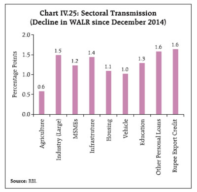
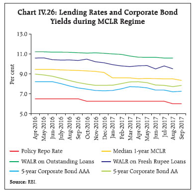
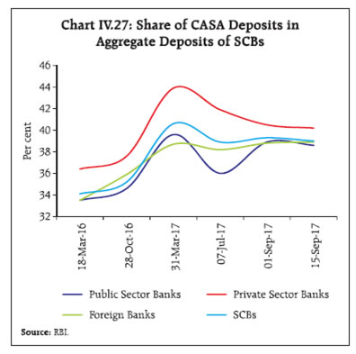 The overall experience with the transmission of monetary policy since the switch over to the MCLR regime from the base rate in April 2016 has not been fully satisfactory. Therefore, as indicated in the Statement on Developmental and Regulatory Policies of August 2, 2017, an internal Study Group (Chairman: Dr. Janak Raj) was constituted by the Reserve Bank to study various aspects of the MCLR system from the perspective of improving monetary transmission. The Study Group, which submitted its report on September 25, 2017, observed that internal benchmarks such as the base rate/MCLR have not delivered effective transmission of monetary policy. Arbitrariness in calculating the base rate/MCLR and spreads charged over them has undermined the integrity of the interest rate setting process. The base rate/MCLR regime is also not in sync with global practices on pricing of bank loans. The Study Group has, therefore, recommended a switchover to an external benchmark in a time-bound manner. (Please see the Report of the Study Group for further details). IV.3 Liquidity Conditions and the Operating Procedure of Monetary Policy The amended RBI Act 1934 requires the Reserve Bank to place the operating procedure relating to the implementation of monetary policy and changes thereto from time to time, if any, in the public domain. The RBI’s approach to managing persistent large surplus liquidity in the post-demonetisation period using a mix of conventional and unconventional instruments was presented in the Monetary Policy Report of April 2017. Anticipating that surplus liquidity conditions may persist through 2017-18, the RBI provided forward guidance on liquidity in April 2017: (a) variable reverse repo auctions with a preference for longer term tenors to be used as the key instrument for absorbing the remaining post-demonetisation liquidity surplus; (b) issuances of T-Bills and dated securities under the MSS up to ₹1 trillion; (c) issuances of CMBs of appropriate tenors of up to ₹1 trillion in accordance with the memorandum of understanding (MoU) with the Government of India to manage enduring surpluses due to government operations; (d) open market operations with a view to moving system level liquidity to neutrality; and (e) fine tuning reverse repo/repo operations to modulate day-to-day liquidity. | Table IV.4: Interest Rates on Small Savings Instruments for Q3: 2017-18 | | (Per cent) | | Small Saving Scheme | Maturity (years) | Spread $ (Percentage point) | Average G-sec yield (%) of corresponding maturity (Jun to Aug 2017) | Formula based rate of interest (%) (applicable for Oct to Dec 2017) | GoI announced rate of interest (%) (applicable for Oct- Dec 2017) | Difference (Percentage point) not transmitted | | (1) | (2) | (3) | (4) | (5) = (3) + (4) | (6) | (7) = (6) - (5) | | Savings Deposit | - | - | - | - | 4.00 | -0.00 | | Public Provident Fund | 15 | 0.25 | 6.70 | 6.95 | 7.80 | 0.85 | | Term Deposits | | | | | | | | 1 Year | 1 | 0 | 6.17 | 6.17 | 6.80 | 0.63 | | 2 Year | 2 | 0 | 6.25 | 6.25 | 6.90 | 0.65 | | 3 Year | 3 | 0 | 6.32 | 6.32 | 7.10 | 0.78 | | 5 Year | 5 | 0.25 | 6.48 | 6.73 | 7.60 | 0.87 | | Post Office Recurring Deposit Account | 5 | 0 | 6.32 | 6.32 | 7.10 | 0.78 | | Post Office Monthly Income Scheme | 5 | 0.25 | 6.44 | 6.69 | 7.50 | 0.81 | | Kisan Vikas Patra | 115 Months | 0 | 6.70 | 6.70 | 7.50 | 0.80 | | NSC VIII issue | 5 | 0.25 | 6.63 | 6.88 | 7.80 | 0.92 | | Senior Citizens Saving Scheme | 5 | 1.00 | 6.48 | 7.48 | 8.30 | 0.82 | | Sukanya Samriddhi Account Scheme | 21 | 0.75 | 6.70 | 7.45 | 8.30 | 0.85 | $ Spreads for fixing small saving rates as per GoI Press Release of Feb 2016.
Note: GoI decided to keep interest rates on small saving schemes for Q3:2017-18 unchanged. | In pursuance of this mandate, the Reserve Bank auctioned T-Bills (tenors ranging from 312 days to 329 days) aggregating ₹1 trillion under the MSS in April and May 2017. Incremental expansion in currency in circulation due to rapid remonetisation drained about ₹2 trillion of surplus liquidity during Q1 of 2017-18. However, this was more than offset by front-loaded expenditure by the Government and large redemption of Government securities. The average daily absorption of liquidity increased to ₹4,562 billion (including LAF, MSS and CMBs) during Q1 of 2017-18 from ₹3,141 billion at end-March 2017 (Chart IV.28). In Q2, frequent recourse to WMAs and ODs by the Government augmented market liquidity even as currency in circulation absorbed up to ₹569 billion. In addition to regular 7-day, 14-day and 28-day variable rate reverse repo auctions, the Reserve Bank conducted open market operations to absorb ₹600 billion on a durable basis (₹200 billion each in July, August and September). With the Government’s cash balance position improving during August, the net average daily absorption of liquidity declined from ₹5,126 billion (including LAF, MSS and CMBs) in the first week of August to ₹4,417 billion by end-August 2017. With advance tax outflows in mid-September, the government cash balances increased to about ₹1,322 billion. Consequently, the surplus liquidity in the system declined to ₹2,771 billion by end-September. The combining of conventional and unconventional instruments into a pro-active liquidity management strategy could have been influential in averting potential risks to inflation, both upside and downside (Box IV.2). 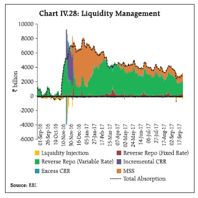
Box IV.2: Managing the Post-demonetisation Liquidity Glut: Minimising Risks to Inflation A causal relationship running from excess liquidity in the banking system to inflation draws from the Friedmanesque proposition: “inflation is always and everywhere a monetary phenomenon”. For modern central banks conducting monetary policy by setting interest rates consistent with the price stability objective, monetary expansion is endogenous – the operating procedure that fully accommodates demand for liquidity (or demand for bank reserves) to keep the overnight money market rates aligned to the policy rate internalises the central bank’s balance sheet. In the face of inadequate credit demand, there has been an involuntary build-up of excess reserves in the banking system since November 2016 reflecting the return of specified bank notes (SBNs) as deposits with banks. Pro-active liquidity management ensured that the WACR did not fall significantly below the LAF floor under the pressure of the resulting liquidity glut. 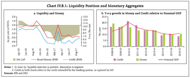 The variable that congeals all lead information about inflation is the monetary aggregate (or broad money), not central bank liquidity that only squares the daily system level mismatch. In fact, even though the net liquidity surplus [as percentage of net demand and time liabilities (NDTL)] in India has been persistently high since demonetisation, broad money (M3) and bank credit growth in the system have remained subdued (Chart IV.B.1). Thus, inflationary pressure could have emerged only if, illustratively, banks had leveraged on easing liquidity to expand credit at a rate faster than the growth in nominal GDP, leading to higher demand for money and stronger growth in broad money. A similar dynamic appears to be playing out under quantitative easing. Advanced economies, in fact, experienced deflation risks despite large surpluses of liquidity sloshing around (Reis, 2016). In the literature, empirical evidence shows that excess liquidity has stoked equity price inflation (Balatti et al, 2017). It has also been found, however, that the dynamic effects of excess liquidity shocks on inflation and asset prices may depend on the state of the economy, in particular, on the state of the business cycle, the credit cycle, the starting position in the inflation and asset price cycles and the monetary policy stance (Baumeister et al, 2008). Drawing on this empirical literature, two vector auto-regression (VAR) models were used with four variables each, taking into account the frequency of data availability. While daily data covering the period from July 2010 to July 2017 are used in the first model (daily net LAF as proportion to banks’ NDTL; daily changes in the spread of the WACR over the effective Fed funds rate, daily changes in the BSE Sensex; and daily net FPI inflows into equity), monthly data covering the period from January 2011 to July 2017 are used in the second model (monthly change in net LAF as proportion to NDTL; spread of the WACR over the repo rate; annualised m-o-m changes in the headline CPI index; and annualised m-o-m changes in broad money as the four variables). All variables used in the two models are stationary, and the VAR lag length is determined by the standard Akaike information criterion/Schwarz information criterion. 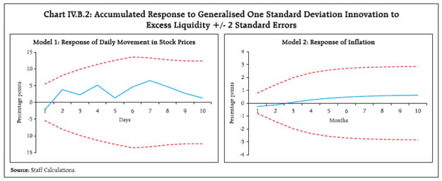 Impulse response functions suggest that excess liquidity does not have a statistically significant impact on the paths of either equity price changes or CPI inflation (Chart IV.B.2). However, a standard deviation shock to broad money (i.e., an increase) is found to be inflationary, as expected. This reflects that when excess liquidity does not lead to higher money growth, it is not inflationary. An exogenous shock to liquidity in the model does not cause either broad money growth to increase or interest rates to fall. It is, therefore, not surprising that post-demonetisation surplus liquidity has not had any impact on inflation in India so far. References Mirco Balatti, Chris Brooks, Michael P. Clements and Konstantina Kappou (2017), “Did Quantitative Easing only inflate stock prices? Macroeconomic evidence from the US and UK”, www.efmaefm.org/0EFMAMEETINGS/.../papers/EFMA2017_0227_fullpaper.pdf. Christiane Baumeister, Eveline Durinck, Gert Peersman (2008), “Liquidity, Inflation and Asset Prices in a Time-Varying Framework for the Euro Area”, https://www.nottingham.ac.uk/cfcm/documents/workshops/baumeister-durinck-peersman.pdf Ricardo Reis (2016), “Funding Quantitative Easing to Target Inflation”, September
https://www.kansascityfed.org/~/media/files/publicat/sympos/2016/econsymposium-reis-paper.pdf?la=en | With remonetisation, currency in circulation has steadily moved closer to the pre-demonetisation level (Chart IV.29), reaching about 88 per cent of the level (₹17.97 trillion) prevailing around the immediate pre-demonetisation period. Looking forward, surplus liquidity conditions are likely to persist in the second half of 2017-18, which will test the goals and instrumentation of the Reserve Bank’s liquidity management framework in its resolve to align the operating target of monetary policy – the WACR – with the policy repo rate and to enable the seamless evolution of other rates in the money market spectrum. Equity and bond markets will likely have to contend with volatility from investor sentiment shifts in response to both global and domestic factors. In the forex market too, the outlook for capital flows and the likely path of the US dollar would interact with domestic fundamentals and the current account deficit to impinge on fair values of the exchange rate and deviations therefrom. A robust revival in credit growth hinges on resolution of stressed assets in the banking system, early and adequate recapitalisation of public sector banks, and a durable pick-up in private investment demand. Ongoing efforts to determine a suitable external benchmark for bank lending rates should bring greater transparency in due course in the setting of interest rates by banks and help improve monetary policy transmission. 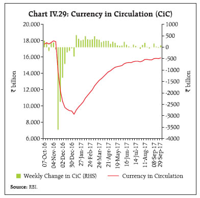
V. External Environment Global growth has broadened to encompass several advanced and emerging market economies. World trade has also picked up and is likely to outpace global GDP growth. Inflationary pressures remain subdued across geographies, supported by soft commodity prices. Since the MPR of April 2017, global growth has strengthened, spreading to several AEs and some commodity exporting EMEs as well, lifting the latter out of recession. Global trade has been buoyed by gradually firming demand, and exports and imports have risen in several economies. Crude prices have firmed up in Q3 on the easing supply glut. Metal prices have rallied, fuelled by resurgent Chinese demand, but have moderated in recent weeks. Growing risk appetite for financial assets led to a fall in bullion prices to multi-month lows, before a recent rally in September. Inflation remains below target levels in many AEs and subdued across several EMEs. International financial markets have been buoyed by these global growth prospects and the accommodative monetary policy stance in major AEs. Financial markets have remained resilient to geo-political events and more recently to the US Fed’s decision to reduce the size of its balance sheet. Equity markets rallied in most AEs, while some correction has been witnessed in a few EMEs. Bond yields in major AEs hardened on expectations of monetary policy normalisation, but generally declined in EMEs with softening inflation and neutral or accommodative policy rates. The US dollar weakened to a multi-month low in September, while the euro rallied further. Movements in EME currencies were mixed but with a general tendency to appreciate. V.1 Global Economic Conditions The US economy expanded at a solid pace in Q2 after a weak performance in Q1. Buoyant labour market conditions, upbeat consumer confidence, softer than expected inflation and a robust housing market supported consumer spending. Industrial production showed an upswing, while non-residential investment growth made a turnaround. Retail sales and business spending suggest that the growth momentum has been sustained in early Q3. However, recent hurricanes could temporarily weigh on economic activity. In the Euro area, economic recovery has gained traction and broadened across constituent economies. GDP growth in Q2 improved over and above the relatively strong outturn in Q1. Unemployment fell consistently, and retail sales rose, lifting both business and consumer sentiment. Strengthening external demand and receding political uncertainty in the region supported the recovery. In Japan, economic expansion accelerated in Q2 from its modest pace in the previous five quarters. Domestic demand – both consumption and investment – rose to a three-year peak. In spite of a weak currency and stronger global demand, net exports turned negative as imports rose, indicating resilient domestic activity. Industrial production accelerated and the labour market steadily tightened, even as financial conditions remained highly accommodative (Table V.1). | Table V.1: Real GDP Growth (q-o-q, annualised) | | (Per cent) | | Country | Q2-2016 | Q3-2016 | Q4-2016 | Q1-2017 | Q2-2017 | 2017 (P) | 2018 (P) | | Advanced Economies (AEs) | | Canada | -1.4 | 4.1 | 2.7 | 3.7 | 4.5 | 2.5 | 1.9 | | Euro area | 1.2 | 2.0 | 2.4 | 2.0 | 2.4 | 1.9 | 1.7 | | Japan | 2.0 | 0.9 | 1.6 | 1.2 | 2.5 | 1.3 | 0.6 | | South Korea | 3.6 | 2.0 | 2.0 | 4.4 | 2.4 | 2.7 | 2.8 | | UK | 2.0 | 1.6 | 2.4 | 1.2 | 1.2 | 1.7 | 1.5 | | US | 2.2 | 2.8 | 1.8 | 1.2 | 3.1 | 2.1 | 2.1 | | Emerging Market Economies (EMEs) | | Brazil | -1.6 | -2.3 | -1.8 | 4.1 | 1.0 | 0.3 | 1.3 | | China | 7.6 | 7.2 | 6.8 | 5.2 | 6.8 | 6.7 | 6.4 | | Malaysia | 4.4 | 5.6 | 5.2 | 7.2 | 5.2 | 4.5 | 4.7 | | Mexico | 0.4 | 4.2 | 2.9 | 2.6 | 2.3 | 1.9 | 2.0 | | Russia* | -0.5 | -0.4 | 0.3 | 0.5 | 2.5 | 1.4 | 1.4 | | South Africa | 3.1 | 0.4 | -0.3 | -0.6 | 2.5 | 1.0 | 1.2 | | Thailand | 3.8 | 2.0 | 2.1 | 5.3 | 5.4 | 3.0 | 3.3 | | Memo: | 2016E | 2017P | 2018P | | World Output | 3.2 | 3.5 | 3.6 | | World Trade Volume | 2.3 | 4.0 | 3.9 | E : Estimate, P : Projection, *: GDP y-o-y.
Sources: Bloomberg and IMF. |
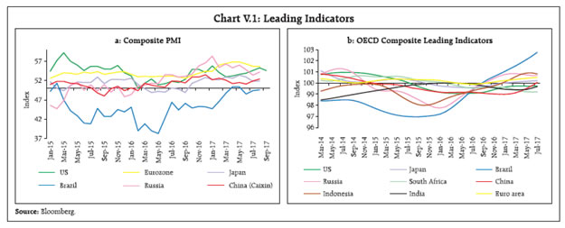 Among EMEs, some convergence in growth dynamics took place during H1:2017 as the economic performance of large commodity exporting economies and of several middle-income countries picked up. In China, growth regained some lost momentum in Q2, supported by fiscal stimulus and growing global demand. However, investment slowed down as lending costs rose and the property market cooled off, though manufacturing continued to expand in spite of tighter financial conditions. China’s debt-fuelled growth remains a potential source of financial instability, triggering a rating downgrade by S&P Global Ratings for the first time since 1999. The Brazilian economy expanded for two consecutive quarters in Q2, but growth dynamics remained fragile due to the depressed labour market and political uncertainty. The Russian economy emerged out of two years of recession, supported by the strengthening global environment and improving macroeconomic fundamentals. Middle-income Asian economies such as Indonesia, Malaysia and Thailand improved their growth performance during H1:2017, riding on stronger demand at home and from abroad. Growth in South Korea, which has risen markedly in Q1, decelerated in Q2 due to a sharp fall in Chinese tourism following a heightening of geopolitical tensions. South Africa exited recession in Q2, however, it continues to face economic and political challenges. Composite purchasing managers’ indices (PMI) indicate economic growth gaining momentum in the US, Eurozone and China, an ebbing of contractionary forces in Brazil and the rate of expansion slowing in the UK and Russia. The OECD’s composite leading indicators (CLIs) point to prospects of growth gaining momentum in China and Brazil, and stable momentum in the US, Euro area and Japan (Chart V.1). Growth in global merchandise trade volume accelerated in Q2:2017 from the lacklustre performance in 2016. Recent data suggest that this upturn has been broad-based as countries accounting for more than two-thirds of world trade (Brazil, China, EU, India, Japan Russia, and the USA) recorded higher trade activity than a year ago. However, it remains far below its level in 2010 (Chart V.2a). Services trade registered some deceleration in Q2:2017 in major economies (Chart V2.b), except the US. The World Trade Outlook Indicator (WTOI) of the World Trade Organisation (WTO) points to a modest pick-up in global services trade in Q3:2017. According to the WTO, this would crucially depend on the performance of travel, financial and business services, though the recovery in merchandise trade could also provide some impetus. Multilateral organisations, viz., the IMF, the World Bank and the WTO project global trade volume rising in 2017 and 2018. However, major economies could face a tough policy environment with the imposition of Section 301 of US trade law that allows unilateral imposition of tariffs which, in turn, could attract geopolitical and retaliatory repercussions. V.2 Commodity Prices and Global Inflation Global commodity prices were affected by demand and supply imbalances, geopolitical tensions and commodity-specific factors, including weather conditions in respect of agricultural commodities. Commodity prices measured by the Bloomberg commodity index declined by 1.0 per cent during April to September 2017, despite some pick-up in late June-July on the upsurge in Chinese demand. Crude oil prices declined by over 8.0 percent in Q2:2017 on account of high inventories, though supply cuts agreed by the OPEC led to some firming up in May. In late Q3, Brent crude prices hit a two-year high in September due to OPEC cuts, declining US crude oil inventories, adverse climatic conditions and geo-political concerns (Chart V.3). Although the recent hurricanes in the US have not impacted crude and gasoline production, the slowdown in localised refinery activity did cause supply disruptions for a short duration. Base metal prices rose by 10.1 per cent during April to September 2017, led by copper, zinc, nickel, aluminium and tin, while prices of iron declined. Metal prices, particularly of copper, have rallied since mid-July, driven by increased demand from China where production itself was disrupted as a fallout of environmental inspections, however, some moderation was witnessed in recent weeks. Gold and silver prices fell by about 1 per cent and 9 per cent, respectively, during Q2:2017 on increased risk appetite that reduced safe haven demand and also due to the weaker US dollar. During Q3:2017, precious metal prices, particularly of gold, have shown some recovery, hitting a 12-month high as tensions sparked between the US and North Korea.
The Food and Agriculture Organisation (FAO)’s food price index grew by over 2 per cent during Q2:2017, driven predominantly by dairy and meat prices. In contrast, edible oil and sugar price indices declined beginning January 2017. Cereal and sugar prices have started firming up from July (Chart V.4). Soft commodity prices have kept inflation expectations quiescent in most AEs, even as economic activity and job creation have strengthened. Inflation in the US has remained well below the target in 2017. Euro area inflation has remained below the target due to still persisting slack in the labour market, despite the sharp increase in energy prices in August. In Japan, inflation continued to be low at less than 0.5 per cent, though deflationary fears have disappeared (Chart V.5a). Inflationary pressures in EMEs continued to be divergent (Chart V.5b). In China, inflation inched up in Q2 following a significant fall in Q1 and touched a seven-month high in September on account of strong domestic demand and increase in the prices of non-food items. In Russia, inflation fell for the first time below the target of 4 per cent in July, while in Brazil, it touched the lower band of the target of 3 per cent in June. In South Africa, inflation eased during 2017, primarily due to falling food inflation. By contrast, Turkey has continued to face double digit inflation since February 2017, driven by high food, transport and housing prices. Inflation in Indonesia surpassed the target of 4 per cent in Q2 on upward revisions in administered electricity prices and festival-related hikes in food prices; however price pressures have moderated recently.
V.3 Monetary Policy Stance The monetary policy stance has remained accommodative globally, though systemic central banks are increasingly communicating an intent towards policy normalisation. In AEs, the US Fed and Bank of Canada raised policy rates. The US has announced balance sheet normalisation beginning October 2017. Sustained economic expansion and job gains have prompted the US Fed to raise policy rates four times in eighteen months, the last being in June. In its September policy meeting, the ECB kept its policy stance unchanged as inflation remains subdued and reaffirmed continuance of its ultra-easy policy stance. Similarly, the Bank of England kept its policy rate unchanged in August, but sounded hawkish as inflation remained above the target due to a weak currency. The Bank of Japan, however, has continued with its ultra-accommodative stance as inflation has remained low with growth still modest (Chart V.6a). Even though monetary policy stances remained diverse in EMEs, several of them either reduced policy rates or kept them unchanged. In Brazil, the policy rate was cut for the sixth time in a row in 2017 so far, as the inflationary situation improved and remained resilient to political uncertainty, while the currency strengthened. South Africa cut its policy rate for the first time in five years in July as the economy slipped into recession in Q1 while inflation pressures eased. Russia cut its policy rate four times in 2017 so far, to support economic recovery, as inflation continued to decline. Although China has kept key policy rates unchanged since October 2015 to control excessive debt financing, liquidity in the system has been tightened through measures such as open market operations. Chile has kept the policy rate unchanged since the rate cut effected in May to support economic activity. Indonesia cut its policy rate twice in Q3 of 2017 on falling inflation and lower current account deficit. Turkey left its tight monetary policy stance unchanged as inflation remained elevated. By contrast, Mexico raised the policy rate in tandem with the US, given close economic linkages (Chart V.6b). V.4 Global Financial Markets Changing expectations about the course of monetary policy in AEs and improving economic prospects influenced risk perceptions of investors and drove global financial markets. Although markets have remained relatively calm and stable, the unwinding of the expansion in Fed’s balance sheet since the global financial crisis is a potential vortex of tension going forward. With its massive holdings of government and mortgage-backed securities (MBS), the Fed is the most dominant player in the US bond market. Furthermore, a reduction of the Fed’s balance sheet would echo growing confidence in the US economy. In turn, this has some implications for financial markets in EMEs (Box V.1). Box V.1: Implications of Unwinding of US Fed Balance Sheet Three rounds of quantitative easing (QE) in the aftermath of the global financial crisis swelled the Fed’s balance sheet from US$ 0.7 trillion in 2008 to the current level of US$ 4.2 trillion, consisting of government securities of around US$ 2.0 trillion, mortgage backed securities (MBS) of US$ 1.7 trillion and other assets. This has had large spillover effects on EMEs through capital flows, though they remained smaller in countries with better fundamentals (Chen et al., 2014). With the strengthening of economic growth in the US, the Federal Open Market Committee (FOMC) indicated a state-contingent unwinding of the balance sheet in June 2017 and outlined the broad principle: government securities and MBS would be allowed to roll off without reinvesting in a graduated manner, which would translate to an annual average reduction of about US$ 270 billion in government securities and US$ 180 billion in MBS over the next two years. In its meeting held on September 20, 2017, the FOMC announced that it would initiate the balance sheet normalisation programme from October 2017. A reversal of QE may involve standard channels of transmission. First, long-term bond yields could increase due to a rise in the term premium induced by higher supply for bonds, leading to steepening of the yield curve. The rise in bond yields, along with tightening of financial conditions, would lead to portfolio rebalancing from equity and risky assets to bonds. Second, a combination of portfolio substitution, risk aversion and safe haven demand could cause a rise in bond yields in the US which could, in turn, induce large capital outflows from EMEs – the larger the external deficit and debt of a country, the higher could be capital outflows and the resultant currency depreciation vis-à-vis the US dollar. Third, consequent upon reallocation of funds by investors towards AEs, financial conditions in EMEs could tighten. Lower asset prices and increased cost of borrowing could adversely affect balance sheets of corporates and banks in these countries, potentially causing rollover problems on debt issued in international markets. Fourth, the exchange rate regime would play an important role in the spillover to the real economy and domestic financial markets. In the case of India, assuming a symmetric reversal of capital inflows during QE, Patra et al., (2016) found that capital outflows could primarily take place through the portfolio rebalancing channel (about 35 per cent of inflow during QE), followed by the liquidity channel1. A hypothetical exercise assuming Fed balance sheet reduction by about one-third to one-half and impacts that are symmetric to that of QE estimated in Bhattarai et al., (2015) in a Bayesian vector autoregression (BVAR) framework indicates the following: (i) in the US, bond yields could harden in the range of 40-60 bps, while the exchange rate could appreciate by about 1-3 per cent and equity prices could fall by about 4-6 per cent; and (ii) spillovers to financial markets in EMEs (including India) could result in bond yields firming up by 12-18 bps, the effective exchange rate depreciating by 0.3-1.0 per cent and equity prices falling by 2.7-5.3 per cent. An event study based on 20 minutes interval data for a two-day window on September 20, 2017 was conducted to gauge the market reaction to the FOMC announcement of Fed balance sheet normalisation in five select economies, viz., Brazil, India, Indonesia, South Africa and Turkey. Financial market volatility, as measured by the coefficient of variation2 (CV), in various market segments, viz., bond, currency and equity markets in the US and other five economies, increased generally. The immediate effect of the announcement was more pronounced on the bond market in the US, especially for the short tenor securities, while the impact on bond markets in other countries was muted (Chart V.B.1). In currency markets, the impact fell largely on the Turkish lira and the South African rand. The Indian rupee was also impacted to some extent. The impact on other currencies was muted. No significant impact was felt on equity markets. The volatility triggered by the FOMC statement in EMEs was mixed (Chart V.B.2). While volatility in bond markets remained higher on the post-announcement day in Brazil, South Africa and Turkey, it declined in Indonesia. In currency markets, volatility increased in all other countries, barring Turkey, and especially for India. In equity markets, volatility remained higher than the pre-announcement day for all other countries, barring Brazil.
References: Bhattarai, Saroj, Arpita Chatterjee, and Woong Yong Park (2015), “Effects of US Quantitative Easing on Emerging Market Economies”, Federal Reserve Bank of Dallas, Working Paper No. 255. Chen, Jiaqian, Tommaso Mancini-Griffoli, and Ratna Sahay (2014), “Spillovers from United States Monetary Policy on Emerging Markets: Different This Time”? IMF Working Paper WP/14/240. Patra M. D., J. K. Khundrakpam, S. Gangadaran, R. Kavediya and J. M. Anthony (2016), “Responding to QE Taper from the Receiving End”, Macroeconomics and Finance in Emerging Market Economies, 9:2, 167-189. _______________________________________________________________ |
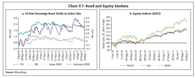 Meanwhile, sovereign bond yields in many AEs rose in recent months, although they remain low by historical standards, given the still low policy rates and term premia suppressed by large assets holdings of central banks. Furthermore, in the US, yields are still trading lower than at the beginning of 2017, as inflation has undershot expectations. In the Euro area, the benchmark 10-year German bond yield rose to a peak level in June as markets began to anticipate the possibility of reversal in monetary easing by the ECB. In the UK, a higher future policy path combined with an inflation rate above target led to a rise in bond yields. In Japan, however, bond yields remained close to zero under the active yield control policy of the Bank of Japan (Chart V.7a). In emerging markets, falling inflation and generally unchanged policy rates led to a fall in yields of local currency denominated bonds. Improvement in economic prospects also led to a softening in bond yields in EMEs as risk premia declined and induced capital inflows into bond markets. Equity prices have risen significantly across economies due to a combination of better global economic prospects, higher corporate earnings and increased risk appetite of investors. The Morgan Stanley Capital International (MSCI) World Index, which measures global equity prices, increased by 8.5 per cent between April and September 2017. Across the world, information technology (IT) share prices have gained the most. Bank share prices have also gained on the back of the rise in long-term government bond yields, which has raised the prospects of banks’ interest earnings. In the US, the Fed’s favourable stress test results further boosted share prices of banks. Similarly, in the Euro area, bank share prices were helped by national reform programmes undertaken by the European Commission. In Japan, a rally in share prices during 2017 was driven by stronger economic performance and higher corporate earnings, partly due to a weaker currency and a lower corporate tax. Equity prices in EMEs gained even more on the positive outlook on economic growth. The gain has been particularly notable for emerging Asia, largely driven by equity prices of IT firms (Chart V.7b). Currency markets were driven by expectations that monetary policy in some AEs would become less accommodative. However, the US dollar continued to depreciate against several currencies since Q1:2017, despite the raising of the policy rate by the Fed in June (Chart V.8a). On the other hand, the euro appreciated significantly against the US dollar and the Japanese yen, driven by a change in the forward guidance of the ECB on reviving economic conditions and marked reduction in political uncertainty. The Japanese yen has continued to fluctuate against the US dollar, but with a depreciating bias, driven by movements in 10-year government bond yield differentials between these two countries. 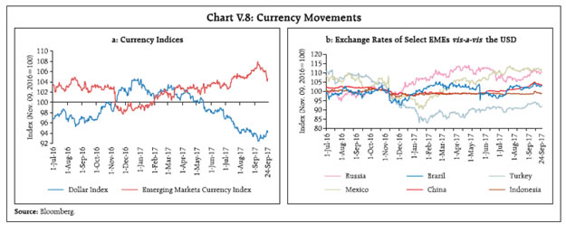 In EMEs, currency movements against the US dollar have been mixed, with country-specific factors playing a significant role (Chart V.8b). The Russian ruble, which strengthened in Q1, depreciated in Q2 due to falling crude oil prices. The Brazilian real depreciated sharply in Q2 and shed all the gains during Q1, following domestic political developments, but recouped in Q3. Most other EME currencies appreciated against the US dollar on surges of capital inflows driven by varied factors such as stronger macroeconomic fundamentals (China, Thailand and emerging European economies); search for yields (South Africa where fundamentals remained weak); and easing of border tensions (Mexico). In sum, a cyclical global economic recovery has gained some momentum which could likely be sustained in 2017. While economic growth has firmed up in some major AEs, it is also showing a turnaround in EMEs. Although inflation pressures remain contained, the recent uptick in commodity prices pose an upside risk. The monetary policy stance will likely shift towards normalisation in major AEs and will be a critical factor in shaping the behaviour of global financial markets with concomitant implications for EMEs.
ABBREVIATIONS | AEs | Advanced Economies | | ARCH | Autoregressive Conditional Heteroscedasticity | | ARDL | Autoregressive Distributed Lag | | ARIMA | Autoregressive Integrated Moving Average | | AUM | Assets Under Management | | BE | Budget Estimates | | BK | Baxter-King | | bps | Basis Point | | BSE | Bombay Stock Exchange | | BVAR | Bayesian VAR | | CAD | Current Account Deficit | | CASA | Current Account and Saving Account | | CBLO | Collateralised Borrowing and Lending Obligation | | CCIL | Clearing Corporation of India Ltd. | | CD | Certificate of Deposit | | CF | Christiano-Fitzqeraled | | CGA | Controller General of Accounts | | CII | Confederation of Indian Industry | | CLI | Composite Leading Indicator | | CMBs | Cash Management Bills | | CMIE | Centre for Monitoring Indian Economy | | CP | Commercial Paper | | CPB | Central Planning Bureau | | CPC | Central Pay Commission | | CPI | Consumer Price Index | | CPI-AL | Consumer Price Index for Agricultural Labourers | | CPI-IW | Consumer Price Index for Industrial Workers | | CPI-RL | Consumer Price Index for Rural Labourers | | CRAR | Capital to Risk Weighted Assets Ratio | | CRR | Cash Reserve Ratio | | CSO | Central Statistics Office | | CU | Capacity Utilisation | | CV | Coefficient of Variation | | DEA | Digestive Enzymes and Antacids | | DGCI&S | Directorate General of Commercial Intelligence and Statistics | | DISCOMs | Distribution Companies | | DSGE | Dynamic Stochastic General Equilibrium | | ECB | European Central Bank | | ECBs | External Commercial Borrowings | | ECM | Error Correction Model | | EMDEs | Emerging Market and Developing Economies | | EMEs | Emerging Market Economies | | EU | European Union | | FAO | Food and Agriculture Organisation | | FC | Finance Commission | | FCCB | Foreign Currency Convertible Bond | | FCNR | Foreign Currency Non-Resident | | FDI | Foreign Direct Investment | | FI | Financial Institution | | FICCI | Federation of Indian Chambers of Commerce and Industry | | FIMMDA | Fixed Income Money Markets and Derivatives Association | | FMCG | Fast-moving Consumer Goods | | FOMC | Federal Open Market Committee | | FPI | Foreign Portfolio Investment | | FRBM | Fiscal Responsibility and Budget Management | | FY | Financial Year | | GARCH | Generalised Autoregressive Conditional Heteroscedasticity | | GDP | Gross Domestic Product | | GFC | Global Financial Crisis | | GFCE | Government Final Consumption Expenditure | | GFCF | Gross Fixed Capital Formation | | GFD | Gross Fiscal Deficit | | GIC | General Insurance Corporation of India | | GNDI | Gross National Disposable Income | | GNPA | Gross Non-Performing Assets | | GoI | Government of India | | G-Secs | Government Securities | | GST | Goods and Services Tax | | GSTN | Goods and Services Tax Network | | GSTR | Goods and Services Tax Return | | GVA | Gross Value Added | | H1 | First Half of the Year | | H2 | Second Half of the Year | | HDFC | Housing Development Finance Corporation | | HP | Hodrick-Prescott | | HRA | House Rent Allowance | | IBC | Insolvency and Bankruptcy Code | | ICRR | Incremental Cash Reserve Ratio | | IGST | Integrated Goods and Services Tax | | IIP | Index of Industrial Production | | IMD | India Meteorological Department | | IMF | International Monetary Fund | | IND-AS | Indian Accounting Standard | | INR | Indian Rupee | | IOCL | Indian Oil Corporation Limited | | IOS | Industrial Outlook Survey | | IPO | Initial Public Offering | | IRFs | Impulse Response Functions | | ISM | Institute for Supply Management | | LAF | Liquidity Adjustment Facility | | LCR | Liquidity Coverage Ratio | | LIC | Life Insurance Corporation of India | | LPA | Long Period Avarage | | LPG | Liquefied Petroleum Gas | | M3 | Broad Money | | mb/d | Million Barrels Per Day | | MBS | Mortgage Backed Securities | | MCA | Ministry of Corporate Affairs | | MCLR | Marginal Cost of Funds Based Lending Rate | | MIBOR | Mumbai Inter-bank Outright Rate | | MIFOR | Mumbai Inter-bank Forward Offer Rate | | MNREGA | Mahatma Gandhi National Rural Employment Guarantee Act | | m-o-m | Month-on-Month | | MoF | Ministry of Finance | | MoU | Memorandum of Understanding | | MPC | Monetary Policy Committee | | MPR | Monetary Policy Report | | MSCI | Morgan Stanley Capital International | | MSMEs | Micro, Small and Medium Enterprises | | MSP | Minimum Support Price | | MSS | Market Stabilisation Scheme | | MVKF | Multivariate Kalman Filter | | NBFCs | Non-Banking Financial Companies | | NBFCs-D | Deposit-taking NBFCs | | NBFCs-ND-SI | Systemically Important Non-deposit Taking NBFCs | | NCAER | National Council of Applied Economic Research | | NDS-CALL | Negotiated Dealing System-Call | | NDTL | Net Demand and Time Liabilities | | NEER | Nominal Effective Exchange Rate | | NFC | Non-Food Credit | | NHB | National Housing Bank | | NIM | Net Interest Margin | | NPA | Non-performing Asset | | NRE | Non Resident Rupee | | NSDL | National Securities Depository Limited | | NSE | National Stock Exchange | | NSSF | National Small Savings Fund | | ODs | Overdrafts | | OECD | Organisation for Economic Co-operation and Development | | OIS | Overnight Index Swap | | OMOs | Open Market Operations | | OPEC | Organisation of the Petroleum Exporting Countries | | PADO | Public Administration, Defence and Other services | | PCE | Personal Consumption Expenditure | | PFCE | Private Final Consumption Expenditure | | PMI | Purchasing Managers’ Index | | PPAC | Petroleum Planning and Analysis Cell | | PRN | Production Weighted Rainfall Index | | PSBs | Public Sector Banks | | PVBs | Private Sector Banks | | QE | Quantitative Easing | | q-o-q | Quarter-on-Quarter | | RBI | Reserve Bank of India | | REER | Real Effective Exchange Rate | | RHS | Right Hand Side | | RRBs | Regional Rural Banks | | SAAR | Seasonally Adjusted Annualised Rate | | SBNs | Specified Bank Notes | | SCBs | Scheduled Commercial Banks | | SDLs | State Development Loans | | SEBI | Securities and Exchange Board of India | | SIAM | Society of Indian Automobile Manufactures | | SLR | Statutory Liquidity Ratio | | SME | Small and Medium Enterprise | | T-Bill | Treasury Bill | | UDAY | Ujwal DISCOM Assurance Yojana | | UK | United Kingdom | | US | United States | | USD | US Dollar | | VAR | Vector Autoregression | | VAT | Value Added Tax | | VR | Variable Rate | | WACR | Weighted Average Call Money Rate | | WADTDR | Weighted Average Domestic Term Deposit Rate | | WALR | Weighted Average Lending Rate | | WMA | Ways and Means Advances | | WPI | Wholesale Price Index | | WTI | West Texas Intermediate | | WTO | World Trade Organisation | | y-o-y | Year-on-Year | |