2.1 Scheduled Commercial Banks (a) Banking stability map and indicator The banking stability map and indicator present an overall assessment of changes in underlying conditions and risk factors that have a bearing on the stability of the banking sector during a period. Existing methodology has been revised by replacing a few variables (financial ratios) of the existing dimensions, incorporating an additional dimension and changing to equal-weighting. The six composite indices would now represent risk in six dimensions - soundness, asset-quality, profitability, liquidity, efficiency and sensitivity to market risk. Each composite index is a relative measure of risk during the sample period used for its construction, where a higher value would mean higher risk in that dimension. The financial ratios used for constructing each composite index are given in Table 1. Each financial ratio is first normalised for the sample period using the following formula: where Xt is the value of the ratio at time t. If a variable is negatively related to risk, then normalisation is done using 1– Yt. Composite index of each dimension is then calculated as a simple average of the normalised ratios in that dimension. Finally, the banking stability indicator is constructed as a simple average of these six composite indices. Thus, each composite index or the overall banking stability indicator takes values between zero and one. | Table 1: Ratios used for constructing the banking stability map and indicator | | Dimension | Ratios | | Soundness | CRAR # | Nonperforming loans net of provisions to capital | Tier 1 capital to assets # | | | Asset- Quality | Gross NPAs to Total Advances | Provisions to nonperforming loans # | Sub-Standard Advances to Gross NPAs # | Restructured Standard Advances to Standard Advances | | Profitability | Return on Assets # | Net Interest Margin # | Growth in Profit Before Tax # | Interest margin to gross income # | | Liquidity | Liquid Assets to Total Assets # | Liquidity Coverage Ratio # | Customer Deposits to Total Assets # | Non-Bank Advances to Customer-Deposits | | Efficiency | Cost to Income | Business (Credit + Deposits) to Staff Expenses # | Staff Expenses to Total Expenses | | | Sensitivity to market risk | RWA (market risk) to capital | Trading income to gross income | | | | Note: # Negatively related to risk. | (b) Macro stress testing Macro-stress test ascertains the resilience of banks against macroeconomic shocks by assessing the impact of macro shocks on capital adequacy of a set of major scheduled commercial banks (46 banks presently). Macro-stress test attempts to project capital ratios over a one-year horizon, under a baseline and two adverse (medium and severe) scenarios. The macro-stress test framework consists of (i) designing the macro scenarios, (ii) projection of GNPA ratios, (iii) projection of profit after tax (PAT), (iv) projection of sectoral probability of default (PD) and (v) projection of capital ratios. I. Designing Macro Scenarios II. Projection of GNPA ratios GNPA ratios are projected for each of the three bank groups viz; Public Sector Banks (PSBs), Private Sector Banks (PVBs) and Foreign Banks (FBs). Natural logs of GNPA ratios of these bank-groups are modelled using two complementary econometric models viz; (i) Autoregressive distributed lag (ADL) model and (ii) Vector auto regression (VAR) model. The values projected based on both these models are averaged to arrive at the final projections of GNPA ratios for each bank-group. The natural logs of GNPA ratios of each bank group are modelled as follows: II.1 Public Sector Banks II.1b VAR Model Log GNPA ratio of PSBs along with the macro variables viz; Nominal GDP growth and 5-year BBB bond spread are modelled using VAR model of order 1. II.2 Private Sector Banks II.3b VAR Model Log GNPA ratio of FBs along with the macro variables viz; WALR of FBs, Exports-to-GDP ratio, Oil price growth and CPI inflation are modelled using VAR model of order 1. II.4 All SCBs The system-level GNPA ratios are projected by aggregating the bank-group level projections using weighted average with gross loans and advances as weights. The projections are done under the baseline and adverse scenarios. III. Projection of PAT The components of PAT such as, net interest income (NII), other operating income (OOI), operating expenses (OE) and provisions are projected for each of the bank-groups using the following models. III.1 Public Sector Banks III.1.1 Projection of Net Interest Income (NII) NII is the difference between interest income and interest expense. The ratio of NII to total average assets of PSBs is modelled using the following ADL and VAR models and the projected values based on these models are averaged to arrive at the final projections. III.1.1b VAR Model NII-to-total average assets ratio is modelled using VAR model of order 1 together with the variables viz; incremental GNPA ratio of PSBs, NIFTY 50 annual growth rate, 5-year term spread, and incremental interest rate spread of PSBs. III.1.4 Projection of Provisions The ratio of Provisions to gross loans and advances of PSBs is modelled using the following ADL and VAR models and the projected values based on these models are averaged to arrive at the final projections. III.1.4b VAR Model Provisions-to- gross loans and advances ratio is modelled using VAR model of order 2 along with the variables viz; GNPA ratio of PSBs, 5-year term spread and gross fiscal deficit. III.2 Private Sector Banks III.2.1 Projection of Net Interest Income (NII) The ratio of NII to total average assets for PVBs is modelled using the following ADL and VAR models and the projected values based on these models are averaged to arrive at the final projections. III.2.1b VAR Model NII-to-total average assets ratios are modelled using VAR model of order 1 along with the variables viz; GNPA ratio of PVBs, NIFTY 50 annual growth rate and interest rate spread of PVBs. III.2.4 Projection of Provisions The ratio of Provisions to gross loans and advances of PVBs is modelled using the following ADL and VAR models and the projected values based on these models are averaged to arrive at the final projections. III.3 Foreign Banks III.3.1 Projection of Net Interest Income (NII) The ratio of NII to total average assets for FBs is modelled using the following ADL and VAR models and the projected values based on these models are averaged to arrive at the final projections. III.3.4 Projection of Provisions The ratio of Provisions to gross loans and advances of FBs is modelled using the following ADL and VAR models and the projected values based on these models are averaged to arrive at the final projections. III.3.4b VAR Model Provisions-to- gross loans and advances ratios are modelled using VAR model of order 1 together with the variables viz; GNPA ratio of FBs and GDP growth. Projection of PAT for each bank group are derived from the projected values of its components using the following identity: Projection of PAT is made under the baseline and adverse scenarios. The applicable income tax is assumed as 35 per cent of profit before tax, which is based on the past trend of ratio of income tax to profit before tax. The bank-wise profit after tax (PAT) is derived using the following steps: -
For each bank-group, components of PAT are projected under baseline and adverse scenarios. -
Share of components of PAT of each bank (except income tax) in their respective bank-group is calculated. -
For each bank, a component of PAT (except income tax) is projected by applying that bank’s share in the component of PAT on the projected value of that component in the respective bank-group. -
Finally, bank-wise PAT is projected by appropriately applying the aforesaid identity on the projected values of components derived in the previous step. IV. Projection of Sectoral PDs Sectoral PDs of 18 sectors/sub-sectors are modelled using ADL models and are projected for four quarters ahead under assumed baseline as well as adverse scenarios. The 18 sectors are listed in Table 2. | Table 2: List of selected sectors/sub-sectors | | Sr. No. | Sector | Sr. No. | Sector | | 1 | Engineering | 10 | Basic Metal and Metal Products | | 2 | Auto | 11 | Mining | | 3 | Cement | 12 | Paper | | 4 | Chemicals | 13 | Petroleum | | 5 | Construction | 14 | Agriculture | | 6 | Textiles | 15 | Retail-Housing | | 7 | Food Processing | 16 | Retail-Others | | 8 | Gems and Jewellery | 17 | Services | | 9 | Infrastructure | 18 | Others |
V. Projection of Capital Ratios Capital projections are made for each of the 46 banks under baseline and adverse stress scenarios. Capital projections are made by estimating risk-weighted assets (RWAs) using internal rating based (IRB) formula and under the conservative assumption that only 25 per cent of PAT would be transferred to capital funds in the subsequent period, as per the minimum regulatory requirements. The formulae used for projection of CRAR and Common Equity Tier 1 (CET1) capital ratio are given below: PAT is projected using the models listed in the previous section. RWA (others), which is total RWA minus RWA of credit risk, is projected based on average growth rate observed in the past one year. RWA (credit risk) is estimated using the IRB formula given below: IRB Formula: Bank-wise RWAs for credit risk were estimated using the following IRB formula; where, EADi is exposure at default of a bank in the sector i (i=1,2….n). Ki is minimum capital requirement for the sector i which is calculated using the following formula: Capital requirement (Ki) where, LGDi is loss given default of sector i, PDi is probability of default of sector i, N(..) is cumulative distribution function of standard normal distribution, G(..) is the inverse of the cumulative distribution function of standard normal distribution, Mi is average maturity of loans of sector i (which is taken 2.5 for all sectors in this case), b(PDi) is smoothed maturity adjustment and Ri is the correlation of sector i with the general state of the economy. Calculation of both, b(PD) and R depends upon PD. The aforesaid IRB formula requires three major inputs, viz; sectoral PD, EAD and LGD. Here, annual slippage of the sectors are assumed as proxies of sectoral PDs. PD of a particular sector is assumed as the same for each of the 46 selected banks. EAD of a bank for a particular sector is considered as the total outstanding loan (net of NPAs) of the bank in that sector. LGD is assumed as 60 per cent (broadly as per RBI guidelines on ‘Capital Adequacy - The IRB Approach to Calculate Capital Requirement for Credit Risk’) under the baseline scenario, 65 per cent under medium stress scenario and 70 per cent under the severe stress scenario. Using these formulae, assumptions and inputs, the capital ratio of each bank is estimated. The differences between IRB-based capital ratios estimated for the latest quarter and those of the ensuing quarters projected under the baseline scenario and the incremental change in the ratios from baseline to adverse scenarios are appropriately applied on the latest observed capital ratios (under Standardised Approach) to arrive at the final capital ratio projections. (c) Housing Price and Financial Stability – Sensitivity Analysis Sensitivity analysis for house prices has been carried out using data of Residential Asset Price Monitoring Survey (RAPMS), a quarterly survey through which RBI collects data from select scheduled commercial banks (SCBs) and housing finance companies (HFCs) on fresh housing loans sanctioned by them in selected cities during a quarter. I. Following assumptions and calculations have been used for the sensitivity analysis: 1. In order to account for the entire outstanding housing loans, following scaling factor was used for each bank: 2. RAPMS data received from 20 PSBs and PVBs from Q4: 2008-09 till Q4:2021-22 are used for the analysis. 3. The property purchased is the collateral for all the loans. 4. The loan and the EMI due remain constant. 5. There is no default till date i.e. all EMIs for all loans are paid as scheduled. 6. Loan amount outstanding is calculated based on sanctioned amount, EMI, derived rate of interest and time elapsed since inception. 7. The derived rate of interest is calculated based on the loan amount sanctioned, maturity period and EMI. 8. Capital to risk-weighted assets ratio (CRAR) of each bank under a price shock scenario is computed by adjusting both the numerator (capital) and the denominator [risk-weighted assets (RWA)] of CRAR. Initial risk weights are taken as per the RBI circular in vogue at the time of origination of the loans. The following method is attempted to recompute CRAR: (a) Housing loans where the shocked collateral value goes below the loan amount outstanding are subjected to the norms of substandard loans: • Additional provisions and interest loss for one quarter are deducted from the numerator (capital). • For the same loans a part of the additional provisioning is deducted from the denominator New RWA for Delinquent Loans = Old RWA - 0.58 x Additional provisioning RWA density being 0.58. (b) RWA for other loans is estimated by internal rating based (IRB) formula: RWA = K x 12.5 x EAD Exposure at default (EAD) is the loan amount outstanding, and K is the capital requirement for a defaulted exposure given by: N(..) is cumulative distribution function of standard normal distribution, G(..) is inverse of cumulative distribution function of standard normal distribution, M is effective maturity of loans (which is taken as 2.5), bPD is smoothed maturity adjustment and R is correlation of the sector with the general state of the economy. Calculation of both, bPD and R depend upon PD. II. The following process is followed: (d) Single factor sensitivity analysis -Stress testing As a part of quarterly surveillance, stress tests are conducted covering credit risk, interest rate risk, liquidity risk etc. and the resilience of commercial banks in response to these shocks is studied. The analysis is done on individual SCBs as well as on the system level. I. Credit risk (includes concentration risk) To ascertain the resilience of banks, the credit portfolio was given a shock by increasing GNPA ratio for the entire portfolio. For testing the credit concentration risk, default of the top individual borrower(s) and the largest group borrower(s) was assumed. The analysis was carried out both at the aggregate level as well as at the individual bank level. The assumed increase in GNPAs was distributed across sub-standard, doubtful and loss categories in the same proportion as prevailing in the existing stock of NPAs. However, for credit concentration risk (exposure based) the additional GNPAs under the assumed shocks were considered to fall into sub-standard category only and for credit concentration risk (based on stressed advances), stressed advances were considered to fall into loss category. The provisioning requirements were taken as 25 per cent, 75 per cent and 100 per cent for sub-standard, doubtful and loss advances respectively. These norms were applied on additional GNPAs calculated under a stress scenario. As a result of the assumed increase in GNPAs, loss of income on the additional GNPAs for one quarter was also included in total losses, in addition to the incremental provisioning requirements. The estimated provisioning requirements so derived were deducted from banks’ capital and stressed capital adequacy ratios were computed. II. Sectoral Credit Risk To ascertain the Sectoral credit risk of individual banks, the credit portfolios of particular sector was given a shock by increasing GNPA ratio for the sector. The analysis was carried out both at the aggregate level as well as at the individual bank level. Sector specific shocks based on standard deviation(SD) of GNPA ratios of a sector are used to study the impact on individual banks. The additional GNPAs under the assumed shocks were considered to fall into sub-standard category only. As a result of the assumed increase in GNPAs, loss of income on the additional GNPAs for one quarter was also included in total losses, in addition to the incremental provisioning requirements. The estimated provisioning requirements so derived were deducted from banks’ capital and stressed capital adequacy ratios were computed. III. Interest rate risk Under assumed shocks of the shifting of the INR yield curve, there could be losses on account of the fall in value of the portfolio or decline in income. These estimated losses were reduced from the banks’ capital to arrive at stressed CRAR. For interest rate risk in the trading portfolio (HFT + AFS), a duration analysis approach was considered for computing the valuation impact (portfolio losses). The portfolio losses on these investments were calculated for each time bucket based on the applied shocks. The resultant losses/gains were used to derive the impacted CRAR. IV. Equity price risk Under the equity price risk, impact of a shock of a fall in the equity price index, by certain percentage points, on profit and bank capital were examined. The fall in value of the portfolio or income losses due to change in equity prices are accounted for the total loss of the banks because of the assumed shock. The estimated total losses so derived were reduced from the banks’ capital. V. Liquidity risk The aim of the liquidity stress tests is to assess the ability of a bank to withstand unexpected liquidity drain without taking recourse to any outside liquidity support. Various scenarios depict different proportions (depending on the type of deposits) of unexpected deposit withdrawals on account of sudden loss of depositors’ confidence along with a demand for unutilised portion of sanctioned/ committed/guaranteed credit lines (taking into account the undrawn working capital sanctioned limit, undrawn committed lines of credit and letters of credit and guarantees). The stress tests were carried out to assess banks’ ability to fulfil the additional and sudden demand for credit with the help of their liquid assets alone. Assumptions used in the liquidity stress tests are given below: -
It is assumed that banks will meet stressed withdrawal of deposits or additional demand for credit through sale of liquid assets only. -
The sale of investments is done with a haircut of 10 per cent on their market value. -
The stress test is done under a ‘static’ mode. (e) Bottom-up Stress testing: Credit, Market and Liquidity Risks Bottom-up sensitivity analyses for credit, market and liquidity risks were performed by 27 select scheduled commercial banks. A set of common scenarios and shock sizes were provided to the select banks. The tests were conducted using March 2022 data. Banks used their own methodologies for calculating losses in each case. (f) Bottom-up stress testing: Derivatives portfolios The stress testing exercise focused on the derivatives portfolios of a representative sample set of top 20 banks in terms of notional value of the derivatives portfolios. Each bank in the sample was asked to assess the impact of stress conditions on their respective derivatives portfolios. In case of domestic banks, the derivatives portfolio of both domestic and overseas operations were included. In case of foreign banks, only the domestic (Indian) position was considered for the exercise. For derivatives trade where hedge effectiveness was established it was exempted from the stress tests, while all other trades were included. The stress scenarios incorporated four sensitivity tests consisting of the spot USD/INR rate and domestic interest rates as parameters. | Table 3: Shocks for sensitivity analysis | | | Domestic interest rates | | | Overnight | +2.5 percentage points | | Shock 1 | Up to 1yr | +1.5 percentage points | | | Above 1yr | +1.0 percentage points | | | | | Domestic interest rates | | | Overnight | -2.5 percentage points | | Shock 2 | Up to 1yr | -1.5 percentage points | | | Above 1yr | -1.0 percentage points | | | | | Exchange rates | | Shock 3 | USD/INR | +20 per cent | | | | | Exchange rates | | Shock 4 | USD/INR | -20 per cent | 2.2 Primary (Urban) Co-operative Banks Single factor sensitivity analysis – Stress testing Stress testing of UCBs was conducted with reference to the reported position as on March 31, 2022. The banks were subjected to baseline, medium and severe stress scenarios in the areas of credit risk, market risk and liquidity risk as follows: I. Credit Default Risk -
Under Credit Default Risk, the model aims to assess the impact of stressed credit portfolio of a bank on its CRAR. -
Arithmetic mean of annual growth rate was calculated based on reported data of NPAs between 2009 and 2020 of the UCB sector as a whole. -
The annual growth rate was calculated separately for each NPA class (Sub-standard, Doubtful 1 (D1), Doubtful 2 (D2), Doubtful 3 (D3) and Loss assets). This annual growth rate formed the baseline stress scenario, which was further stressed by applying shocks of 1.5 Standard Deviation (SD) and 2.5 SD to generate medium and severe stress scenarios for each category separately. -
Based on the above methodology, the annual NPA growth rate matrix arrived at under the three stress scenarios was as below. These were further adjusted bank wise based on their NPA divergence level. | (per cent) | | | Increase in Substandard Assets | Increase in D1 assets | Increase in D2 assets | Increase in D3 assets | Increase in Loss assets | | Baseline Stress | 25.33 | 19.95 | 17.78 | 12.73 | 34.80 | | Medium Stress | 66.83 | 49.15 | 42.22 | 49.03 | 184.44 | | Severe Stress | 94.50 | 68.62 | 58.52 | 73.23 | 284.20 | II. Credit Concentration Risk It was assumed that under the three stress scenarios the top 1, 2 and 3 single borrower exposures respectively moves from ‘Standard Advances’ category to ‘Loss Advances’ category leading to 100 per cent provisioning and its consequent impact on CRAR. III. Interest Rate Risk in Trading Book -
The duration analysis approach was adopted for analysing upward movement of interest rates on AFS and HFT portfolio of UCBs. -
Due to absence of data with respect to modified duration (MD) for UCBs, the model used the weighted average MD of small finance banks (SFBs) given the structural similarities between SFBs and UCBs, with an increase of 50 basis points as a conservative approach. -
Upward movement of interest rates by 50 bps, 150 bps and 250 bps were assumed under the three stress scenarios and provisioning impact on CRAR was assessed. IV. Interest Rate Risk in Banking Book - The Banking Book of UCBs was subjected to interest rate shocks of 50 bps, 150 bps and 250 bps under three stress scenarios and impact on Net Interest Income was arrived at.
V. Liquidity risk The stress test was conducted based on cumulative cash flows in the 1-28 days’ time bucket. The cash inflows and outflows were stressed under baseline, medium, and severe scenarios as below: | (per cent) | | Stress Scenario | Decrease in Inflows | Increase in Outflows | | Baseline | 5 | 25 | | Medium | 5 | 50 | | Severe | 5 | 100 | The banks with negative cumulative mismatch (cash inflow less cash outflow) exceeding 20 per cent of the outflows were considered to be under stress on the basis of the circular RBI/2008-09/174 UBD. PCB. Cir. No12/12.05.001/2008-09 dated September 17, 2008, which stipulates that the mismatches (negative gap between cash inflows and outflows) during 1-14 days and 15-28-days’ time bands in the normal course should not exceed 20 per cent of the cash outflows in each time band. 2.3 Non-Banking Financial Companies (NBFCs) Stress Testing – Single factor sensitivity analysis Credit and liquidity risks stress tests for NBFCs have been performed under baseline, medium and high risk scenarios. I. Credit risk Methodology for assessing the resilience of NBFC sector to shocks in credit risk has been revised to enhance the model’s accuracy in predicting CRAR under baseline and two stress scenarios. Based on the revised model, assets, advances to total assets ratio, EBPT to total assets ratio, risk weight density and slippage ratio were projected over next one year time period. Thereafter, new slippages, provisions, EBPT, risk weighted assets and capital were calculated for the baseline scenario. For the medium and high risk scenarios, slippages under baseline scenario was increased by 1 SD and 2 SD and accordingly new capital and CRAR were calculated. II. Liquidity Risk Stressed cash flows and mismatch in liquidity position were calculated by assigning predefined stress percentage to the overall cash inflows and outflows in different time buckets over the next one year. Projected outflows and inflows as on March 2022 over the next one year were considered for calculating the liquidity mismatch under baseline scenario. Outflows and inflows of the sample NBFCs were applied a shock of 5 per cent and 10 per cent for time buckets over the next one year for the medium and high-risk scenarios respectively. Cumulative liquidity mismatch due to such shocks were calculated as per cent of cumulative outflows and NBFCs presenting negative cumulative mismatch were identified. 2.4 Interconnectedness - Network analysis Matrix algebra is at the core of the network analysis, which uses the bilateral exposures between entities in the financial sector. Each institution’s lendings to and borrowings from all other institutions in the system are plotted in a square matrix and are then mapped in a network graph. The network model uses various statistical measures to gauge the level of interconnectedness in the system. Some of the important measures are given below: 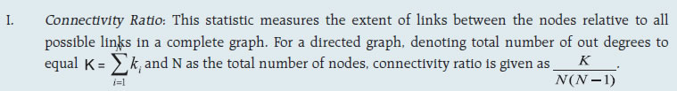 II. Cluster coefficient: Clustering in networks measures how interconnected each node is. Specifically, there should be an increased probability that two of a node’s neighbours (banks’ counterparties in case of a financial network) are neighbours to each other also. A high clustering coefficient for the network corresponds with high local interconnectedness prevailing in the system. For each bank with ki neighbours the total number of all possible directed links between them is given by ki (ki-1). Let Ei denote the actual number of links between agent i’s ki neighbours, viz. those of i’s ki neighbours who are also neighbours. The clustering coefficient Ci for bank i is given by the identity: 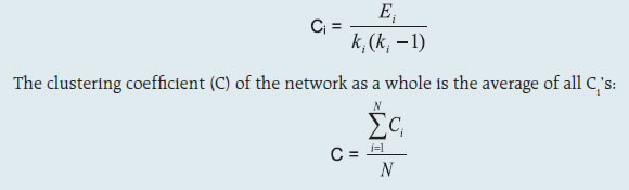 III. Tiered network structures: Typically, financial networks tend to exhibit a tiered structure. A tiered structure is one where different institutions have different degrees or levels of connectivity with others in the network. In the present analysis, the most connected banks are in the innermost core. Banks are then placed in the mid-core, outer core and the periphery (the respective concentric circles around the centre in the diagrams), based on their level of relative connectivity. The range of connectivity of the banks is defined as a ratio of each bank’s in-degree and out-degree divided by that of the most connected bank. Banks that are ranked in the top 10 percentile of this ratio constitute the inner core. This is followed by a mid-core of banks ranked between 90 and 70 percentile and a 3rd tier of banks ranked between the 40 and 70 percentile. Banks with a connectivity ratio of less than 40 per cent are categorised as the periphery. IV. Colour code of the network chart: The blue balls and the red balls represent net lender and net borrower banks respectively in the network chart. The colour coding of the links in the tiered network diagram represents the borrowing from different tiers in the network (for example, the green links represent borrowings from the banks in the inner core). (a) Solvency contagion analysis The contagion analysis is in nature of stress test where the gross loss to the banking system owing to a domino effect of one or more banks failing is ascertained. We follow the round by round or sequential algorithm for simulating contagion that is now well known from Furfine (2003). Starting with a trigger bank i that fails at time 0, we denote the set of banks that go into distress at each round or iteration by Dq, q= 1,2, …For this analysis, a bank is considered to be in distress when its Tier-I CRAR goes below 7 per cent. The net receivables have been considered as loss for the receiving bank. (b) Liquidity contagion analysis While the solvency contagion analysis assesses potential loss to the system owing to failure of a net borrower, liquidity contagion estimates potential loss to the system due to the failure of a net lender. The analysis is conducted on gross exposures between banks. The exposures include fund based and derivatives ones. The basic assumption for the analysis is that a bank will initially dip into its liquidity reserves or buffers to tide over a liquidity stress caused by the failure of a large net lender. The items considered under liquidity reserves are: (a) excess CRR balance; (b) excess SLR balance; and (c) 17 per cent of NDTL. If a bank is able to meet the stress with liquidity buffers alone, then there is no further contagion. However, if the liquidity buffers alone are not sufficient, then a bank will call in all loans that are ‘callable’, resulting in a contagion. For the analysis only short-term assets like money lent in the call market and other very short-term loans are taken as callable. Following this, a bank may survive or may be liquidated. In this case there might be instances where a bank may survive by calling in loans, but in turn might propagate a further contagion causing other banks to come under duress. The second assumption used is that when a bank is liquidated, the funds lent by the bank are called in on a gross basis (referred to as primary liquidation), whereas when a bank calls in a short-term loan without being liquidated, the loan is called in on a net basis (on the assumption that the counterparty is likely to first reduce its short-term lending against the same counterparty. This is referred to as secondary liquidation). (c) Joint solvency-liquidity contagion analysis A bank typically has both positive net lending positions against some banks while against some other banks it might have a negative net lending position. In the event of failure of such a bank, both solvency and liquidity contagion will happen concurrently. This mechanism is explained by the following flowchart: The trigger bank is assumed to have failed for some endogenous reason, i.e., it becomes insolvent and thus impacts all its creditor banks. At the same time it starts to liquidate its assets to meet as much of its obligations as possible. This process of liquidation generates a liquidity contagion as the trigger bank starts to call back its loans. Since equity and long-term loans may not crystallize in form of liquidity outflows for the counterparties of failed entities, they are not considered as callable in case of primary liquidation. Also, as the RBI guideline dated March 30, 2021 permits the bilateral netting of the MTM values in case of derivatives at counterparty level, exposures pertaining to derivative markets are considered to be callable on net basis in case of primary liquidation. The lender/creditor banks that are well capitalised will survive the shock and will generate no further contagion. On the other hand, those lender banks whose capital falls below the threshold will trigger a fresh contagion. Similarly, the borrowers whose liquidity buffers are sufficient will be able to tide over the stress without causing further contagion. But some banks may be able to address the liquidity stress only by calling in short term assets. This process of calling in short term assets will again propagate a contagion. The contagion from both the solvency and liquidity side will stop/stabilise when the loss/shocks are fully absorbed by the system with no further failures. |