The recovery in economic activity remains stimulus dependent. For restoring and recreating a policy environment conducive for private sector-led growth post-COVID, timely rebalancing of monetary and fiscal policies may become necessary given the current configurations of debt and liquidity. Government debt exceeding threshold levels exert upward pressures on the term premium and dampen growth. Time varying fiscal multipliers suggest that fiscal consolidation is not growth retarding once the economy recovers to its steady state. The debt path over the next five years, even under the best-case scenario, may further squeeze fiscal space unless strategic policy efforts covering both taxes and expenditure aim at targeted consolidation. What should be the appropriate monetary-fiscal policy mix in the post-pandemic future becomes a searing existential question for which past behavioural regularities, parametric estimates and analytical received wisdom may not provide adequate guidance.

1. Introduction

II.1 The monetary and fiscal policy response to COVID in India was swift, bold and targeted.¹ Given the enormous scale and wide-ranging nature of the fiscal and monetary stimulus and the overall theme of this report, the post-pandemic macroeconomic policy balance in India will warrant a rethink, in view of the post-COVID debate: liquidity trap limits the effectiveness of monetary policy (Krugman, 2020); fiscal multipliers are large and significantly greater than one during periods of economic slack/high uncertainty (Goemans, 2022); money-financed fiscal stimulus has larger multipliers than debt-financed stimulus (Gali, 2020); excess money injected by central banks is not always inflationary (Stella, 2021); sustainable debt levels are much higher than what one possibly thought earlier (Blanchard, 2022); and secular stagnation – particularly associated with depressed private demand and low interest rate – justifies fiscal activism (Summers and Rachel, 2019). Nevertheless, a large fiscal stimulus in emerging market economies (EMEs) post-COVID could raise the future inflation trajectory. Higher interest rates to deal with such inflation could endanger debt sustainability in a weak growth environment (BIS, 2021).

II.2 Against this backdrop, the key motivations of this chapter are to: (i) assess the impact of fiscal stimulus on growth under different macroeconomic conditions; and (ii) examine the importance of timely rebalancing of crisis-time policies to minimise risks to medium-term growth and inflation. This assessment is done against the backdrop of the existing empirical findings in India which suggest a threshold relationship between debt and GDP (at 40 per cent of GDP for the central government) beyond which further increases in debt become detrimental to growth. For every 0.3 percentage point of GDP increase in the central government’s fiscal deficit or market borrowing, long-term G-sec yields could firm up by 10 bps (or even higher during periods of sharper market reactions) (GOI, 2017). The initial gains in output due to delay in monetary policy response tend to get eroded by the higher than warranted policy reaction later on, eventually resulting in a substantial deterioration in the medium-term output-inflation trade-offs (RBI, 2021c). In the context of these India specific empirical lessons, this chapter highlights that post-COVID, a return to the fiscal-monetary steady state balance could be conducive for both higher growth and lower inflation. The post-COVID period also calls for a revisit of debt sustainability.

II.3 Set against these key motivations, this chapter is organised under five sections. Section 2 examines the effectiveness of fiscal stimulus by estimating the fiscal multipliers associated with different expenditures and their asymmetric impact over the business cycles. Section 3 discusses the lessons learnt from India’s own experience in the past, to draw inferences for post-COVID rebalancing. It deals with three specific empirical issues: (i) the impact of surplus liquidity on inflation; (ii) the threshold level of government debt beyond which term premia and G-sec yields start to harden; and (iii) the relationship between growth and unemployment on one hand and output gap and inflation on the other. Feasible options for public debt consolidation are explored and alternative trajectories for Government debt are evaluated in Section 4. The key policy inferences are summarised in Section 5.

2. Impact of Policy Stimulus on Growth

II.4 The impact of fiscal stimulus on growth can be assessed directly from the components of GDP – i.e., the contributions of government final consumption expenditure (GFCE) and public sector capital formation to GDP growth. A more comprehensive assessment, however, can be conducted through time-varying fiscal multipliers, as the impact materialises over several quarters. In India, increase in public expenditure is found to be more effective than tax cuts whereas for dealing with a situation of economic overheating tax hikes work better than cutbacks in expenditure (Bhat and Sharma, 2021).

II.5 Against this backdrop, using a three-variable structural vector autoregression (SVAR) model (Blanchard and Perotti, 2002) with annual nominal growth in tax revenue, government expenditure and GDP for the period 1981-82 to 2019-20², general government (centre and states combined) fiscal multipliers for total expenditure and its components are estimated with relevant controls.³ The estimated impact multipliers show that only capital expenditure leads to proportionately higher increase in GDP (Table II.1). However, the revenue expenditure and total expenditure multipliers are less than one – in the range of 0.72 to 0.84 – which corroborates the limited effectiveness of fiscal activism in reviving and reconstructing the Indian economy post-COVID. In order to identify conditions under which a fiscal stimulus can be expansionary as opposed to conditions under which fiscal consolidation can be expansionary, time-varying multipliers need to be estimated.

II.6 A smooth transition vector autoregression (STVAR) model⁴ is employed to assess the impact of government expenditure on GDP in the Indian context, which captures non-linearity in the relationship and helps estimate the state-dependent multipliers for regimes of economic expansion and contraction (Auerbach and Gorodnichenko, 2012). The STVAR includes nominal GDP and fiscal variables (total expenditure, capital expenditure and revenue expenditure; one at a time) as the main variables and output gap is taken as the reference variable to define expansion and recession. Given that a sufficiently long time series data are needed to capture the upcycle and downcycle trends, the analysis has been restricted to the Centre only for which quarterly fiscal data are available for a longer time frame.

II.7 Two broad policy inferences could be drawn from the estimated multipliers (Table II.2). First, during a period of economic slack, and a post-crisis situation of sudden collapse in private demand, fiscal stimulus helps in generating growth impulses that amplify through multiplier effects. Capital expenditure is particularly effective in this state of the economy, signifying the importance of quality of public expenditure even in a period of economic slack. Second, in a period of economic expansion, multiplier values turn negative, signifying the detrimental impact of expansionary fiscal policy on growth. Fiscal consolidation, thus, becomes a necessity for allowing the private sector to sustain the growth momentum and mitigating the potential drag on growth from fiscal activism once the economy fully recovers. The need for a credible medium-term fiscal consolidation plan after a crisis to safeguard the medium-term growth trajectory, thus, is corroborated by empirical assessment of the relationship between fiscal expenditure and growth for India.

II.8 In India, a sizable part of the fiscal stimulus during the pandemic was also aimed at incentivising the flow of credit to stressed sectors through collateral free guarantee support and interest rate subventions. Accommodative monetary policy was also pursued alongside, which is likely to have contributed to enhancing the impact of fiscal stimulus as it ensured ample and low-cost liquidity that partly worked through these fiscal incentives. Accordingly, a four variable VAR model – with year-on-year growth in real GDP, CPI inflation (excluding food and fuel items), weighted average call money rate (WACR) and gross fiscal deficit (GFD) of the central government to GDP ratio for the period 1998:Q1 to 2020:Q1 – is estimated which suggests a statistically significant response of growth to both monetary policy and fiscal policy shocks (Chart II.1).⁵ A one percentage point fall in WACR leads to 26 basis points (bps) rise in GDP growth after one quarter and a cumulative impact of 92 bps by the fourth quarter.⁶ On the other hand, the cumulative response of GDP growth to one percentage point rise in GFD-GDP ratio is found to be 43 bps by the fourth quarter.

II.9 The VAR model was further augmented with interactive dummies to ascertain whether fiscal multipliers work symmetrically over the business cycle. The findings suggest that an expansionary fiscal stance works only under economic contraction; during a period of expansion, it does not improve the growth outcome but entails adverse implications for inflation and term premium (as discussed subsequently). In contrast, monetary policy works symmetrically in stabilising output, i.e., it is effective under both expansion and contraction (Chart II.2). These findings corroborate the need for fiscal policy to take the lead in a post-crisis period to support growth, and timely fiscal consolidation to allow monetary policy to effectively stabilise the economy around the steady state during periods of expansion. Hence, as recovery gains further momentum, fiscal consolidation should ideally precede monetary policy normalisation to minimise trade-off costs.

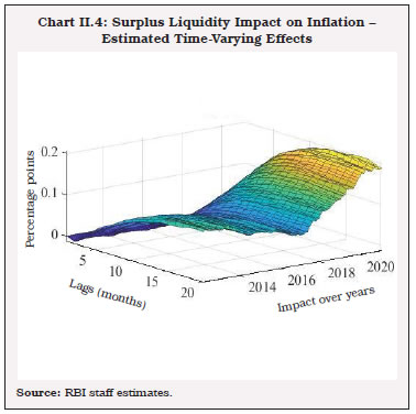
3. Lessons from India’s Own Experience

II.10 The monetary-fiscal policy mix in India was moving into balance consistent with stated objectives preceding the outbreak of COVID-19. Nonetheless, a weakening of the growth momentum since 2017-18 prompted deferment of the fiscal deficit target and use of the escape clause. As regards monetary policy, with average CPI inflation remaining closer to the target, an accommodative stance was adopted since June 2019. Thus, stabilisation policies had retained their focus on reviving growth even ahead of the pandemic.

II.12 The inflationary impact of liquidity is analysed further by using a time-varying parameter VAR (TVP-VAR) model to find out how the impact of liquidity on inflation has evolved over time. The VAR is estimated with inflation, net LAF (as a per cent of NDTL) and WACR as the key variables – using monthly data for the period January 2012-March 2021.⁸ The time-varying impulse responses show that the impact of liquidity is inflationary, with lingering persistence (Chart II.4). Moreover, the impact is largely subdued in the initial phases, but the cumulative impact increases over time. The liquidity impact on inflation in fact appears to have increased over the years. For a one percentage point rise in surplus liquidity (as per cent of NDTL) the peak increase in inflation ranges between 5 to 11 bps up to December 2017. Subsequently, the peak impact is estimated to have increased to about 20 bps. The cumulative impact over about six quarters, however, exceeds 200 bps.⁹ The persistent impact of liquidity on inflation underscores the importance of timely normalisation of systemic surplus liquidity in the post-pandemic period to ward off potential risks to inflation. Even if surplus liquidity initially may not stimulate demand enough to cause inflation, an accommodation of supply-shock induced inflation through persistent excess liquidity can create vicious dynamics in an atmosphere of frequent occurrences of supply side shocks and hardening of inflation expectations.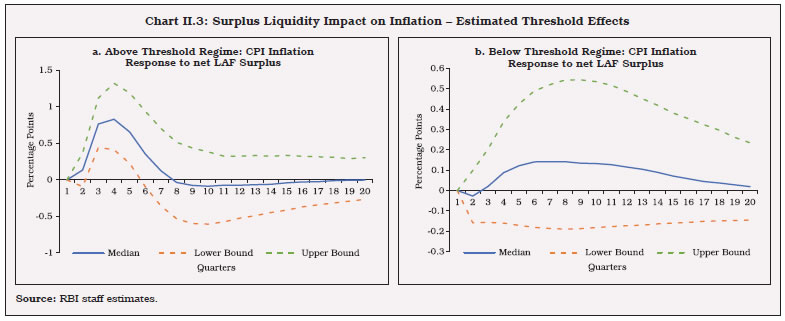

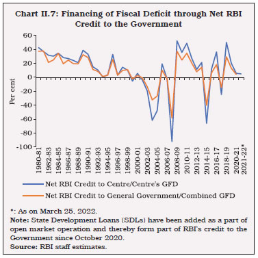
II.13 Estimates using data for the period 1998:Q1 to 2020:Q1 and the same four variables in a VAR as described above suggest that the impact of a policy rate cut (captured through equivalent fall in the WACR) could raise inflation by about 25 bps by the fourth quarter (Chart II.5a). Surplus liquidity reinforces the impact of interest rate cuts on inflation, but with asymmetric effects during different phases of a business cycle. The impulse-response path suggests that a reduction in the policy rate is less inflationary during a slowdown in economic activity than expansion (Chart II.5b).

II.14 Surplus liquidity, and accompanying excess money growth, can be viewed both as an endogenous process of monetary accommodation of the government’s demand for money [through open market operations (OMOs) and G-sec Acquisition Programme (G-SAP), indirectly] and an exogenous money creation process when the central bank proactively injects excess liquidity into the system on its own to promote growth which, in turn, helps in smoother completion of government market borrowings at reasonable interest rates. The space for endogenous indirect accommodation in any normal year in India is influenced by: (a) the required increase in primary money consistent with growth in nominal GDP, and (b) the extent of automatic increase in primary money that results from net accretion to RBI’s foreign assets. With the share of foreign assets in the RBI’s balance sheet rising with the progressive liberalisation of the economy and surges in capital flows, the scope for indirect accommodation has fallen steadily as the share of domestic assets (acquired through open market purchases) has declined (Chart II.6a). During years when capital inflows are large, the entire increase in reserve money may result through expansion in net foreign assets (NFA), leaving no space for indirect accommodation of the fiscal requirements in monetary policy operations. In fact, there are several years when the RBI has had to undertake sterilisation operations [i.e., conduct open market sales or reduction in net domestic assets (NDA)] to offset the excessive expansion in reserve money due to increase in foreign assets (Chart II.6b).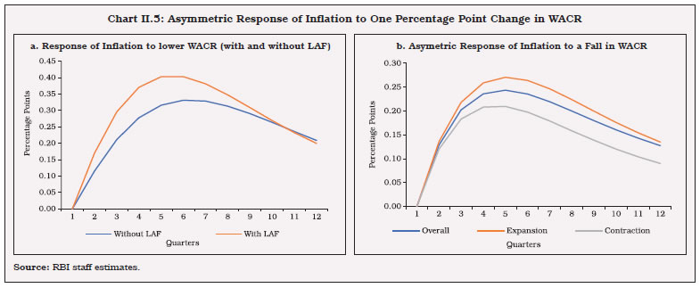

II.15 Reflecting the above dynamics, indirect accommodation of fiscal deficit through RBI credit to the Government (as percentage of gross fiscal deficit) has fluctuated over time, with a recent peak of about 50 per cent in respect of the central government (Chart II.7).

II.16 Post-COVID, indirect accommodation was ensured through a combination of open market purchases, higher ways and means advance (WMA) limits in 2020-21, and G-SAPs as an additional instrument in H1:2021-22. Market absorption of fiscal deficit was also facilitated through the provision of ample system level liquidity and higher held to maturity (HTM) regulatory flexibility for banks. As a result, despite the record high size of the consolidated fiscal deficit (13.3 per cent of GDP), the cost of borrowings for the central government fell to a 17-year low in 2020-21 (Chart II.8).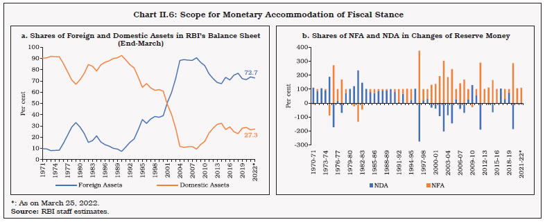

II.17 Despite fiscal consolidation in 2021-22, longer term yields witnessed sporadic and larger than warranted deviations from the policy repo rate. While concerns relating to inflation and external spillovers largely influenced short-term movements in yields, it was the overhang of high fiscal deficit and government debt that exerted sustained upward pressures on longer-term yields. It is important in this context to assess the threshold level of debt beyond which the term premium starts moving up significantly.

II.18 In standard forward-looking debt sustainability analysis, a country/region specific risk premium is often added to the interest rate outlook. When debt levels exceed a threshold level of 60 per cent of GDP for the European countries, risk premium rises by about 4 bps (as per the IMF thumb rule) and 3 bps (as per the European Commission thumb rule) for every percentage point increase in debt-to-GDP ratio (Alcidi and Gros, 2018). A 10-percentage point increase in debt to GDP ratio can thus increase term premium by about 30 to 40 bps. Since the financing cost for corporates and businesses is linked to sovereign risk premium, a high level of government debt can depress growth – an expansionary fiscal policy at high levels of debt can become effectively contractionary (Alcidi and Gros, 2019; Mohanty and Panda, 2020). In India, an impact assessment suggests that when the central government debt exceeds a threshold value of 55 per cent of GDP, every one percentage point increase in the debt to GDP ratio causes the term premium to harden by about 22 bps in the short-run and the impact could increase to as high as 56 bps in the long-run (Box II.1).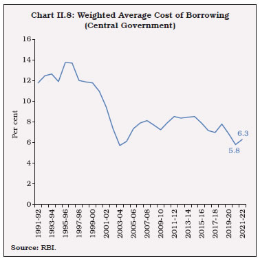

II.19 A dynamic latent factor model, augmented with macroeconomic variables representing real activity, inflation, policy rate, global uncertainty and government market borrowing along with net LAF, is estimated to study the impact of liquidity on term premium or slope of the yield curve, following Diebold et al. (2006). Within the modelling framework, term premium has been extracted from the g-sec yields of maturities of 2 to 10 years, and then regressed on the macroeconomic variables. The Bayesian impulse response results suggest that a one percentage point increase in net LAF (as per cent of NDTL) results in a reduction in term premium by 16 bps (Chart II.9). The increase in liquidity has a sobering effect across the yield curve, but with a relatively higher impact on longer-term rates. By reducing risk premium, the injection of liquidity flattens the yield curve.

Box II.1 Debt Impact on Risk Premium In view of the sharp increase in fiscal deficit and debt in India following the response to the pandemic, an attempt is made to assess whether there is any threshold level of debt beyond which an increase in debt impacts term premia significantly. A standard two regime smooth transition regression of the following form is estimated (Teräsvirta, 1994): 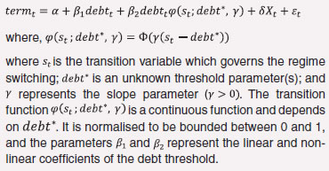A quarterly model is used to estimate the impact of debt on term premium by regressing term premia (termt; defined as the difference between 10-year G-sec yields and 3-month treasury bill yields) on a constant and central government debt to GDP ratio (debtt), while controlling for other determinants of term premia, viz. inflation deviation from the target (Inf_gap), net LAF as percentage of NDTL (LAF), output gap (ygap) and two dummy variables to capture the outlier effects of the taper tantrum (dtaper) and the global financial crisis (dgfc). The estimated results show that there exists a nonlinear relationship between term premia and debt, and debt has differential effects on term premia beyond the threshold level of 55 per cent of GDP (as against actual debt level of 59.1 per cent of GDP as at end-March 2022). The term premium increases by about 22 bps for each one percentage point increase in the debt to GDP ratio above the threshold of 55 per cent (Table 1). Following the fiscal response to the pandemic, the central government debt level has gone up, but term premia did not harden as much as the estimates would suggest, which is because of the strong downward pull from large surplus liquidity. If the debt level continues to remain high for long, any closing of the output gap or normalisation of liquidity, or both, could raise term premium by up to 56 bps in the long-run. Table 1: Estimated Parameters (Sample: 2004Q1 - 2021Q1)   Coefficient t-statistics Threshold: debt* 54.85*** 33.57 Slope: γ 0.66 1.52 Variable     debt < debt* -21.32* -1.98 debt > debt* 21.73* 1.76 termt-1 0.62*** 10.17 Inf_gapt 12.68*** 3.44 ygapt -7.52*** -2.82 LAFt -13.54*** -2.82 dtaper -202.86*** -5.18 dgfc -121.12*** -2.98 R2 0.88   LM(4) P-val 0.48   ARCH(4) P-val 0.81   ***, **; *: Significant at less than 1 per cent, 5 per cent and 10 per cent levels, respectively. Reference: Teräsvirta, T. (1994). Specification, Estimation, and Evaluation of Smooth Transition Autoregressive Models. Journal of the American Statistical Association, 89(425), 208-218.

II.20 It is perhaps prudent to step into a post-pandemic world with the sobering lessons from the recent experience that the salubrious impact of fiscal actions on growth can potentially be offset by higher inflation. Both fiscal discipline and effective management of the second order effects of supply side pressures on inflation are essential for achieving macroeconomic stability which will lay the foundation for monetary policy’s endeavour to set a post-pandemic path of strong, broad-based and sustainable growth. In this context, the renewal of the tryst with fiscal prudence that is the defining feature of the Union Budget 2022-23 is a step in the right direction, especially the strategy of placing less emphasis on linear time-invariant GFD reduction and focusing on the reprioritisation of expenditure in a manner that is growth-friendly and non-inflationary. The challenge for the setting of monetary policy is the continued pursuit of an accommodative stance even as the fiscal impulse is being withdrawn especially in an environment in which persisting pressures from repetitive supply shocks threaten to undermine the credibility of the central bank. What should be the appropriate monetary-fiscal policy mix in the post-pandemic future becomes a searing existential question for which existing behavioural regularities, parametric estimates and analytical received wisdom may not provide adequate guidance.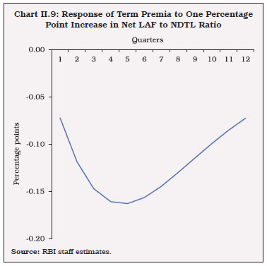

II.21 Empirical estimates in this section indicate that achieving a regime of low inflation and low cost of capital that is conducive to growth and investment is also contingent upon normalisation of liquidity and consolidation of debt over the medium-run. The pragmatic way forward in the post-COVID rebalancing of monetary and fiscal policies is to proceed with the existing state of knowledge on the mix while being prepared for course corrections and innovations as the path evolves.

II.22 One regularity of the pre-pandemic past could be Okun’s Law or the expected inverse relationship between GDP growth and unemployment rate (Ball et al., 2017). Estimates of the Okun’s coefficient across geographies range from (-)0.1 to (-)0.8 – a one percentage point decline in GDP growth may raise the unemployment rate by 0.1-0.8 percentage points. For India, the data on unemployment rate and real GDP growth from 1980-81 to 2019-20¹⁰ suggest that a decline in GDP growth by one percentage point increases unemployment rate by around 0.13 percentage points.¹¹ This is corroborated by evidence from the results based on periodic labour force survey (PLFS) data (Srija and Singh, 2021). In a post-pandemic environment, however, stability of the estimated parameter cannot be presumed, and permanent scarring effects on the labour market cannot be ruled out.

II.23 The output gap (both in level and changes) is a commonly used proxy of economy-wide slack/ tightness associated with cycles of economic activity (Chart II.10). A New Keynesian Phillips Curve (NKPC) estimated on seasonally adjusted quarterly data for the period 1996-97:Q1 to 2019-20:Q4 of the form:

suggests that closing the output gap by one percentage point can raise inflation by about 20 bps with a lag of seven quarters. There is also evidence of a speed limit effect - rapid changes in economic activity may cause larger changes in the inflation rate for a given level of the economic activity (Jose et al., 2021). Inflation expectations (captured by inflation trend or survey-based expectations) also play a role in influencing actual inflation outcomes in India.¹³ Thus, while coordinated fiscal-monetary policy stimulus is necessary to revive growth, delayed normalisation can potentially increase inflation alongside or even ahead of economic recovery.

4. Post-COVID Debt Overhang: Debt Consolidation for Stronger Economic Growth

II.24 General government debt in India surged to 89.4 per cent of GDP in 2020-21 (Chart II.11), significantly higher than the FRBM target of 60 per cent, posing risks to medium-term macroeconomic stability. Hence, an exploration of paths along which India’s public debt may evolve in the medium-term, based on alternative feasible scenarios for real GDP growth, inflation, interest rate and the primary deficit is desirable in order to derive the threshold level of debt beyond which it may become a drag on GDP growth.

II.25 In a post-COVID world, there is likely to be intellectual support for tolerating higher government debt on the ground of a favourable interest rate - growth differential (Blanchard et al, 2021, GOI, 2021). It is important to keep in perspective, however, that the behaviour of primary balances also matters from the point of view of generating fiscal space to pay down the debt – the sufficient condition for debt sustainability. Accordingly, a credible and viable debt management for post-pandemic times will warrant a reordering of strategy. The desirable condition of debt sustainability needs to be a path of reduction of primary deficits to balance or even a modest surplus that spreads out consequent output losses so as to minimise the cost of consolidation. The sufficient condition could be satisfied by committing upfront to reprioritising expenditure in favour of those heads that are growth enhancing and hence, qualitatively superior so that the Domar condition (g>r)¹⁴ is always satisfied. Country-specific features need to condition the assessment of tolerable level of government debt reduction, including the share of interest payments and other committed expenditure in GDP as a measure of the flexibility for manoeuvre. In India, interest payment on the stock of central and state government debt is high by international standards (more than one-fifth of total expenditure) – a drag on debt consolidation (Chart II.12).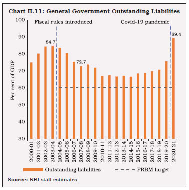

II.26 Monetary policy can help debt consolidation by keeping nominal interest rates/ costs of borrowings low for current/future debt, but that is possible only in a low inflation environment.

II.27 It is against this backdrop that feasible scenarios for India are evaluated under forward looking debt projections in the equation given below¹⁵:

If the real interest rate exceeds real GDP growth (r - g > 0) then the debt to GDP ratio can only increase further, unless it is compensated by a primary surplus.¹⁶ In India, (r - g) has consistently remained favourable in the last three decades. The debt to GDP ratio, however, actually increased during the 2010s despite negative (r - g) (Chart II.13). Starting with a debt level of 89.4 per cent of GDP in 2020-21, the best consolidation efforts in the future (primary deficit of 1.5 per cent of GDP by 2026-27) and most feasible/realisable favourable (r - g) outcomes could still keep the debt to GDP ratio above 75 per cent of GDP over the next five years, higher than in any year during the decade preceding the pandemic (Box II.2).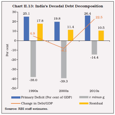

Box II.2 Limits to Consolidation of Public Debt in India Post-Pandemic Public debt is regarded as sustainable when the primary balance needed to stabilise the debt, under both baseline and realistic shock scenarios, is economically and politically feasible and the level of debt is consistent with an acceptably low rollover risk (IMF, 2021). The debt-stabilising level of primary balance (pbt*) is given by the following equation: This implies that countries which have a negative interest rate-growth differential (IRGD) can run a primary deficit and still have sustainable debt. In India, except for a few years, the IRGD has been consistently negative, even though its magnitude has decreased significantly over the last two decades. Historically, several debt crises have occurred globally after years of low and negative IRGD as marginal interest rates rise sharply and abruptly only a few months ahead of a default (Mauro and Zhou, 2020). Besides, debt beyond a certain threshold poses several risks viz., the interest rate on public debt increases with the debt level (Laubach, 2009). High debt countries face significant risk premia that may create a feedback loop in which high-risk premia result in higher debt, which, in turn, leads to even higher risk premia (Alcidi and Gros, 2019). Furthermore, countries with higher public debt experience a larger increase in interest rate in response to a positive growth shock and adverse global volatility shocks (Presbitero and Wiriadinata, 2020). Table 1: Debt Dynamics Tool – Key Assumptions and Results   Historical Projection (Baseline) 2015-16 2016-17 2017-18 2018-19 2019-20 2020-21 2021-22 2022-23 2023-24 2024-25 2025-26 2026-27 Real GDP Growth 8.0 8.3 6.8 6.5 3.7 -6.6 8.9 7.2 6.6 6.3 6.2 6.1 GDP Deflator Inflation 2.3 3.2 4.0 3.9 2.4 5.6 9.7 6.0 5.0 4.5 4.0 4.0 Gross Primary Balance -2.2 -2.2 -1.1 -1.1 -2.5 -7.8 -4.8 -3.8 -3.3 -2.8 -2.5 -2.2 Nominal Effective Interest Rate 7.8 7.7 7.7 7.5 7.1 7.1 7.1 7.1 7.1 7.1 7.1 7.1 Debt (Per cent of GDP) 68.5 68.8 69.8 70.7 75.7 89.4 85.2 84.3 84.2 83.9 83.8 83.6 Note: 1. Real GDP growth for 2021-22 and 2022-23 are based on NSO advance estimates and RBI projections, respectively. 2023-24 onwards projections are based on World Economic Outlook (October 2021). 2. GDP deflator inflation for 2021-22 is based on NSO’s advance estimates of nominal and real GDP. 3. A declining path of gross primary deficit is assumed in line with the union government’s gradual fiscal consolidation plan of reaching GFD-GDP ratio of 4.5 per cent by 2025-26 and Fifteenth Finance Commission’s indicative deficit path for states. Based on the IMF’s recently released Debt Dynamics Tool, India’s general government debt path is projected for the period 2021-22 to 2026-27. The historical values and baseline assumptions on GDP growth, inflation, primary balance and effective interest rate are set out in Table 117. In the baseline scenario the general government debt is assessed to contract steadily to reach 83.6 per cent of GDP by 2026-27. An analysis of debt-creating flows shows that in the projection period, debt stabilisation rests entirely on GDP growth as shocks to both primary deficit and interest rate add to the debt stock (Chart 1a). After moderating in 2021-22, debt is likely to remain sticky at around 84 per cent of GDP over the next five years (Chart 1b). To assess stress scenarios, a 0.5 standard deviation shock (individually) is given to real GDP, primary balance and interest rate in 2022-23, which lasts until 2023-24. The results show that a real GDP shock has the maximum adverse impact as debt shoots up to 86.6 per cent of GDP in the terminal year of projection, as against 83.6 per cent in the baseline scenario. An interest rate shock has only a modest impact on the projected debt path (Chart 2a). 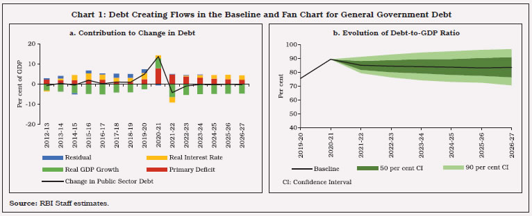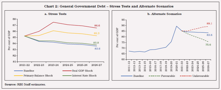In addition to the baseline scenario, we also explore both favourable and unfavourable scenarios incorporating feedback effects which work along with individual shocks. In the favourable scenario, GDP growth is assumed at 8 per cent from 2023-24 onwards, associated with slightly higher inflation (which supports debt consolidation) and primary balance is assumed to be lower than the baseline scenario (through targeted efforts at consolidation). In this setting, the general government debt is assessed to contract to 75.6 per cent of GDP by 2026-27. In the unfavourable scenario, growth is assumed to stagnate at 5 per cent of GDP from 2023-24 onwards. The primary balance and inflation are assumed to be same as in the baseline scenario. In this case, debt changes its declining trajectory after 2021-22 and expands to 89.1 per cent of GDP by 2026-27 (Chart 2b). References: Alcidi, C. and Gros, D. (2019), “Public Debt and the Risk Premium: A Dangerous Doom Loop”, CEPS Policy Insights, No. 2019-06. IMF (2021), “Review of the Debt Sustainability Framework for Market Access Countries”, IMF Policy Paper, International Monetary Fund, January. Laubach, T. (2009), ';New Evidence on the Interest Rate Effects of Budget Deficits and Debt';, Journal of the European Economic Association, 7(4), 858-885. Mauro, P. and Zhou, J. (2020), “r-g < 0 : Can We Sleep More Soundly?” IMF Economic Review, 69(1), 197-229. Presbitero, A. and Wiriadinata, U. (2020), “The Risk of High Public Debt Despite a Low Interest Rate Environment” VOXEu.org, August 5.

II.28 Turning to threshold effects in India, an empirical estimate of the relationship between debt and economic growth for India found the threshold level of general government debt to be 61 per cent (Kaur and Mukherjee, 2012).

II.29 The following regression in quadratic form is estimated for the period from 1981-82 to 2019-20, controlling for real investment growth, trade (growth in sum of real non-oil exports and imports) and the gross fiscal deficit (as per cent of GDP):

where, GDP is the growth in real gross domestic product at market prices; DEBT is the general government outstanding liabilities as per cent of GDP; INVEST is the growth in real fixed investment; TRADE is the growth in sum of real non-oil exports and imports; GFD is the central government’s gross fiscal deficit as a per cent of GDP; and ε_t is the error term.

II.30 The results find that accumulation of general government debt up to a level of 66 per cent of GDP, leads to an increase in GDP growth beyond which it impacts growth adversely (Table II.3). In fact, GDP growth may decline by 0.01 percentage points for one percentage point increase in debt/GDP ratio once the debt level exceeds 66 per cent, with the impact magnifying with higher level of debt.

II.31 This calls for adoption of bold and innovative ways to rebuild fiscal space. The government has launched the National Monetisation Pipeline (NMP) with an aggregate monetisation potential of ₹6 lakh crore, over a four-year period, 2021-22 to 2024-25, making it co-terminus with the balance period of the National Infrastructure Pipeline (2019-20 to 2024-25). Asset monetisation can potentially solve the twin problems of management of existing assets by tapping private sector efficiencies and financing of new infrastructure by unlocking the value of investment made in public assets which have not yielded appropriate or potential returns so far (Kant, 2021). Furthermore, the funds received by the government are proposed to be used for creation of new infrastructure which could generate substantial multiplier effects, bridge existing infrastructure gaps, and lead to inclusive socio-economic development. Beyond innovative financing options and reorientation of expenditure towards capex to benefit from higher multiplier effects, rationalisation of expenditure and raising the country’s tax to GDP ratio may have to be an integral part of the fiscal rebalancing act post-COVID.

5. Conclusion

II.32 The recovery in economic activity remains stimulus dependent, even as new risks to growth and inflation have emerged from the war in Ukraine and normalisation of monetary policy in the US. For restoring and recreating a policy environment conducive for private sector-led growth post-COVID, timely rebalancing of monetary and fiscal policies may become necessary given the current configurations of debt and liquidity.

II.33 First, large surplus liquidity that helped financial conditions to ease significantly during COVID needs to be withdrawn in a calibrated manner. This is because when surplus liquidity persists at above 1.5 per cent of NDTL, for every percentage point increase in surplus liquidity, the average inflation could rise by about 60 basis points in a year. Surplus liquidity within the threshold of 1.5 per cent of NDTL, however, is found to pose no significant risks to inflation. Since inflation exceeding a threshold of 4-6 per cent is inimical to growth¹⁹, adequate supply-side measures to contain inflation should be the priority rather than passive monetary accommodation through ample surplus liquidity.

II.34 Second, empirical estimates suggest term premium coming under pressure once the central government debt exceeds a threshold level of about 55 per cent of GDP. While surplus liquidity is found to have a significant sobering effect on term premium, easy liquidity should not be a policy instrument to raise the tolerable level of debt in the economy. Moreover, when general government debt exceeds another critical threshold level of about 66 per cent, it is found to dampen growth.

II.35 Third, the scenario analysis suggests that even under best possible macroeconomic outcomes, general government debt may not decline to below 75 per cent of GDP over the next five years. If adverse scenarios materialise, in fact, debt may increase. A medium-term transparent strategy of debt consolidation aimed at reducing general government debt to below 66 per cent of GDP at the earliest would be important to secure the medium-term growth prospects of India.

II.36 Fourth, fiscal consolidation is unlikely to be growth retarding, as the time varying fiscal multipliers for India suggest. Once the economy returns to steady state, fiscal multipliers can change from greater than one during a crisis to less than one or even negative. The debt path over the next five years, even under the best-case scenario, will further squeeze fiscal space unless strategic policy efforts covering both taxes and expenditure aim at targeted consolidation, without relying perpetually on the wobbly comfort from a favourable interest rate minus growth condition of debt sustainability.

II.37 With monetary policy prioritising price stability and pursuing output stabilisation in an environment in which debt sustainability is sought to be achieved by fiscal prudence, the assignment rule is satisfied bringing in its train macroeconomic stability to support sustainable growth.

References

Alcidi, C. and Gros, D. (2018), “Debt Sustainability Assessments: The State of the Art”, Economic Governance Support Unit Directorate-General for Internal Policies of the European Union (PE 624.430), November.

Alcidi, C. and Gros, D. (2019), “Public Debt and the Risk Premium: A Dangerous Doom Loop”, CEPS Policy Insights, No. 2019-06.

Auerbach, A. J., and Gorodnichenko, Y. (2012), “Measuring the Output Responses to Fiscal Policy”, American Economic Journal: Economic Policy, 4(2), 1-27.

Ball,L., Leigh, D. and Loungani P. (2017), “Okun’s Law: Fit at 50?”, Journal of Money, Credit and Banking, 49(7), 1413-1441.

Bhat, J. A., and Sharma, N. K. (2021), “Asymmetric Fiscal Multipliers in India–Evidence from a Non-Linear Cointegration”, Macroeconomics and Finance in Emerging Market Economies, 14(2), 157-179.

BIS (2021), Annual Economic Report 2021, Bank for International Settlements.

Blanchard, O. (2022), Fiscal Policy under Low Interest Rates, MIT Press.

Blanchard, O., Felman, J. and Subramanian, A. (2021), “Does the New Fiscal Consensus in Advanced Economies Travel to Emerging Markets?”, Policy Brief, Peterson Institute for International Economics, 21-7, March.

Blanchard, O., and Perotti, R. (2002), “An Empirical Characterization of the Dynamic Effects of Changes in Government Spending and Taxes on Output”, The Quarterly Journal of Economics, 117(4), 1329-1368.

GOI (2021), Economic Survey of India 2020-2021, Government of India.

------ (2017), FRBM Review Committee, Government of India.

Diebold, F. X., Rudebusch, G. D., and Aruoba, S. B. (2006), “The Macroeconomy and the Yield Curve: A Dynamic Latent Factor Approach”, Journal of Econometrics, 131(1-2), 309-338.

Galí, J. (2020), “The Effects of A Money-Financed Fiscal Stimulus”, Journal of Monetary Economics, 115, 1-19.

Goemans, P. (2022), “Historical Evidence for Larger Government Spending Multipliers in Uncertain Times than in Slumps”, Economic Inquiry, https://doi.org/10.1111/ecin.13068

Jose, J., Shekhar, H., Kundu, S., Kishore, V., and Bhoi, B. B. (2021). “Alternative Inflation Forecasting Models for India – what Performs Better in Practice?”, Reserve Bank of India Occasional Papers, 42 (1), 71-121.

Kant, A. (2021), “The Asset Monetisation Dividend”, The Financial Express. January 05, 2021. https://www.financialexpress.com/opinion/the-asset-monetisation-dividend-amitabh-kant/2164284/

Kaur, B., and Mukherjee, A. (2012), “Threshold Level of Debt and Public Debt Sustainability: The Indian Experience”, Reserve Bank of India Occasional Papers, 33(1-2), 1-29.

Krugman, P. (2020), “Liquidity Trap Has Spread to Emerging Markets”, Bloomberg May 12, 2020. https://www.bloombergquint.com/politics/krugman-says-the-liquidity-trap-has-spread-to-emerging-markets

Mohanty, R. K., and Panda, S. (2020), “How Does Public Debt Affect the Indian Macroeconomy? A Structural VAR Approach”, Margin: The Journal of Applied Economic Research, 14(3), 253-284.

Patra, M. D. (2022), “RBI’s Pandemic Response: Stepping out of Oblivion”, Keynote Address delivered at the C D Deshmukh Memorial Lecture Organised by the Council for Social Development, Hyderabad on January 28, 2022.

Primiceri, G. E. (2005), “Time Varying Structural Vector Autoregressions and Monetary Policy”, The Review of Economic Studies, 72(3), 821-852.

RBI (2021a). Annual Report 2020-21, Reserve Bank of India, March.

------(2021b). Report on Trend and Progress of Banking in India 2020-21, Reserve Bank of India, December.

------(2021c). Report on Currency and Finance 2020-21, Reserve Bank of India, February.

Srija, A. and Singh, J. (2021), “How Reliable is Labour Market Data in India? PLFS vs CMIE”, Economic and Political Weekly, 56(52), 21-23.

Stella, P. (2021), “Interpreting Modern Monetary Reality”, Journal of Applied Corporate Finance, 33(4), 8-23.

Summers, L. H., and Rachel, L. (2019), “On Falling Neutral Real Rates, Fiscal Policy and the Risk of Secular Stagnation”, In Brookings Papers on Economic Activity BPEA Conference Drafts, March.

This chapter has been prepared by Sitikantha Pattanaik, Harendra Behera, Binod B. Bhoi, Sangita Misra, Saksham Sood, Sujata Kundu and Ranajoy Guha Neogi. The team is grateful to Dr. Michael Debabrata Patra for his helpful comments and suggestions.

¹ These measures have been comprehensively documented in RBI (2021a; 2021b) and Patra (2022).

² The estimation is restricted to pre-COVID period as unprecedented variation in many key macroeconomic variables due to the COVID shock could have disturbed the empirical relationship.

³ Following the literature, control variables used for the estimation are: global growth, changes in exchange rate (Indian rupees per USD), weighted average call money rate (WACR), government debt to GDP ratio and change in Sensex, with appropriate lags. The results are robust under the unit root and the auto-correlation tests. The impact multiplier is derived by taking the ratio of the coefficient to the share of government expenditure in GDP (Blanchard and Perotti, 2002).

⁵ The effectiveness of fiscal policy is further confirmed by extending the VAR estimation to cover the pandemic period (i.e., 2020:Q2 through 2021:Q1); fiscal policy is found to have contributed to growth revival in the presence of an accommodative monetary policy.

⁶ The estimates are worked out by normalising impulse responses to a one percentage point fall in WACR and a one percentage point rise in GFD-GDP ratio.

⁹ The inflation impact is found to be statistically significant after six months but persists thereafter for long.

¹⁰ Data on unemployment rate are collected from the International Labour Organisation (ILO) and data for a few missing years are intercalated using linear interpolation.

¹² where, π_t is difference in log CPI (i.e., q-o-q change), X_t is a measure of economic activity represented by output gap [(actual output minus potential output)/potential output*100], Δ (X_t) is the change in the output gap, and Z_t is a vector of supply side factors (minimum support prices, nominal exchange rate, global non-fuel commodity prices and rainfall deviation); E_tπ_t+1 is the expected future inflation (which is proxied by lagged inflation trend and 1-year ahead inflation expectations of households) and ε_t is the white noise term. Potential output is measured by the Hodrick-Prescott filter method. In equation (1), the coefficients of the inflation term on the right-hand side are assumed to sum up to unity, implying the existence of a vertical long-run Phillips curve. Additionally, a set of quarterly dummy variables has been used as controls in the estimation.

¹⁴ g_t is the real GDP growth rate and r_t is the real interest rate.

¹⁵ d_t is the debt to GDP ratio; r_t is the real interest rate; g_t is the real GDP growth rate; pb_t is the primary balance and dda_t is deficit-debt adjustment or the stock-flow adjustment comprising factors that affect debt but are not included in the budget balance (Alcidi and Gros, 2018).

¹⁶ A key aspect of any forward-looking exercise on debt sustainability is the projection of primary balances or fiscal efforts required/feasible to stabilise debt. Unlike the simple static view presented in the above equation, in real life all key variables in the equation may be endogenous, with the relationship likely to be also both asymmetric and time-variant. For example, discretionary fiscal efforts directed at containing primary deficit may impact growth, interest rate and inflation. Fiscal multipliers being sensitive to the state of the business cycle, as mentioned earlier, the endogenous impact on other variables could vary over time. Moreover, any change in debt can also generate positive/negative spillback effects on growth, inflation and interest rate. The emphasis on a forward-looking approach in such analyses may also require taking a view on post-COVID possible trend shifts in the potential growth path and the equilibrium real interest rate.

¹⁷ Given that India’s external debt is less than 3 per cent of GDP and around 5 per cent of total debt, we have assumed that entire government debt is held domestically for this exercise.

¹⁸ DUM08 is a dummy variable to capture the effects of global financial crisis and DUM91 is another dummy variable to capture the effects of balance of payments crisis in India on GDP growth.

¹⁹ See RBI (2021c) for details.