Press Release RBI Working Paper Series No. 04 Macroeconomic Forecasting in India:Does Machine Learning Hold the Key to Better Forecasts? Bhanu Pratap, Shovon Sengupta* Abstract #Forecasting of macroeconomic indicators is a challenging task, compounded by complex processes and dynamic nature of the macroeconomy. With recent advancements in computing power and the advent of data, machine learning methods have been explored as an alternative to traditional forecasting methods. We review the paradigm of machine learning and apply it to forecast inflation for India. We train various machine learning algorithms and test their forecasting accuracy against standard statistical methods. Our findings suggest that machine learning methods are generally able to outperform standard statistical models. Further, we find that combining forecasts from different competing models improves forecasting accuracy when compared to individual model forecasts. Also, direct forecast of headline inflation provides better forecast than the forecast based on different components of inflation. Lastly, our analysis also finds preliminary evidence for stochastic seasonality in the inflation series for India. JEL Classification: C22, C45, C52, E37 Keywords: Time series, forecasting, machine learning, deep learning, inflation Introduction Macroeconomic forecasters have traditionally relied upon two different approaches – structural and non-structural (Diebold, 1998). The structural approach is guided by economic theory for model specification while the non-structural approach focuses on exploiting the specific properties of the underlying data without explicitly relying on any economic theory. Non-structural models attach more importance to predictive accuracy over causal inference and are useful for short-term unconditional forecasting. Time-series models, like the univariate autoregressive integrated moving average (ARIMA) or the multivariate vector autoregression (VAR) models, are usually the preferred non-structural models (Pescatori and Zaman, 2011). Linearity in parameters is the key assumption of such time-series models. However, as it was observed during the 1980s and 1990s, linear models failed to identify macroeconomic business cycles, periods of extreme volatility and regime changes which led non-linear models to gain more attention (Sanyal and Roy, 2014). More recently, machine learning (ML) algorithms have also been proposed in the literature on forecasting as an alternative to statistical models. With the advancement in computation and availability of high-frequency data, a considerable amount of research is focusing on utilising ML methods (especially Neural Network [NN] models) for time-series predictions, methodological advancements and accuracy improvements (Makridakis et al., 2018a). While both statistical and ML models aim at improving prediction accuracy by minimising a loss function, they differ in terms of their approach to minimise the loss function – the former uses linear processes and the latter depends on non-linear algorithms. Yet, the much-claimed superiority of ML models over statistical models cannot be taken as given (Zhang, 2007; Makridakis et al., 2018a). This is largely an empirical question which needs to be tested carefully and likely depends on the target indicator, underlying data generating process (DGP), forecast horizon and data quality. Additionally, new developments are taking place across sectors with the emergence of ‘Big Data’, so much so that data is called the new oil (The Economist, 2017). Applications of Big Data and ML-based analytics are also increasingly being used by central banks. Large central banks have embarked on establishing their own data analytics teams with the aim to tackle key issues related to market regulation, supervision, surveillance, risk management and monetary policymaking (Chakraborty and Joseph, 2017). For central banks, such advancements call for addition of newer tools to their analytical toolkit – ones which are adept at handling large volume, high-frequency data. In the Indian context, the Reserve Bank of India (RBI) formally adopted a flexible inflation targeting (FIT) regime in 2016. Given the forward-looking nature of monetary policy, forecasts of inflation play an important role in policy formulation. In this paper, we review various state-of-the-art ML algorithms with the aim to familiarise the readers with this alternative approach to predictive modelling. We select consumer price index (CPI) inflation and three of its components as target variables for our forecasting exercise. CPI-based inflation is chosen because it is a target for monetary policy, published regularly with a high frequency, and is subject to relatively fewer revisions. After introducing various statistical and ML models, we use them to generate forecasts for all four series of inflation and compare these forecasts with those from our benchmark model. Resultant out-of-sample forecasts are compared using standard measures of forecast accuracy. Additionally, we analyse two related issues in the context of forecasting inflation – first, combination of forecasts from different competing models; second, comparative approaches of directly forecasting headline inflation versus forecasting each component and combining them to generate a final forecast for headline inflation. The key findings of our paper are as follows. First, ML methods generally outperformed standard statistical methods over the out-of-sample forecast period. Second, simple average-based forecast combination outperformed complex weighted average combination of forecasts. Such forecast combination also provided better forecasting accuracy over individual methods in almost all cases. Third, directly forecasting headline inflation resulted in large accuracy gains over the approach of individually forecasting and combining inflation components, for any given forecasting method. In fact, forecasts based on a combination of best performing methods for each component also did not perform better than direct forecasts. To our knowledge, very few studies have explored the application of ML techniques to model or forecast inflation in India (Malhotra and Maloo, 2017; Pradhan, 2011; Rani et al., 2017). We also highlight several key features of the ML approach which may result in accuracy gains when adopted for modelling and forecasting using econometric techniques. The rest of the paper is organised as follows. Section II highlights evidence on the performance of ML-based forecasting methods in predicting macroeconomic and financial time-series indicators. We also discuss the findings from various rounds of the Makridakis Competitions, an international series of large-scale forecasting competitions being organised since 1982. In Section III, we briefly review the various statistical and ML models used in the paper, in addition to discussing the data, modelling and evaluation strategy. Results from the forecasting exercise are presented in Section IV. We conclude with a summary of findings and chart out the scope for future research in Section V. II. Machine Learning, Makridakis Competitions and Empirical Evidence II.1. Machine learning as a forecasting approach   A logical starting point for the ML approach to forecasting would be to understand model complexity and the trade-off between bias and variance – the two main sources of forecast error. Errors due to inappropriate assumptions about the data are attributed to bias, while variance of a model describes errors due to a model’s sensitivity to changes in the data. Both bias and variance are dependent on model complexity in such a manner that there exists a trade-off between the two. A model with low bias, high variance will fit a complex model on the data but will tend to generate poor forecasts due to overfitting. A model with high bias, low variance will fit a simple model on the data but will tend to generate poor forecasts due to underfitting. The trade-off between bias and variance and its relationship with model complexity is shown in Chart 1. The ML approach to forecasting aims to find an optimum balance between bias and variance of a model to simultaneously achieve low bias and low variance. In general, any application of ML algorithms would begin with a specification of the task at hand, for example, the prediction of y given a predictor x. The next step is to train (estimate) a model with the objective to minimise a loss function (e.g. mean squared error or MSE) using a subsample of the data containing both y (label) and x (feature) called the ‘training set’. The training involves several iterations using the training set to ‘learn’ from the data. Once the model is trained, it is tested on the ‘test set’, a subsample of data that was not shown to the model earlier. Upon evaluation against the test set, the model is further fine-tuned through ‘tuning’ or adjusting various components of the model such as hyperparameters1, the number of times the model is trained on the training data, initial weights, data transformation and so on. Finally, the predictions are obtained using the final model selected. II.2. Makridakis Competition and Empirical Evidence on ML-based Forecasting The Makridakis Competitions (or M-Competitions) are a series of open competitions intended to evaluate and compare the accuracy of different forecasting methods. Such large-scale open competitions, which include participation from academicians and industry practitioners alike, have proved to be a fertile ground for testing out various empirical questions related to forecasting. The first round of the M-competition was organised in 1982 and the latest M4-Competition concluded in May 2018. In the first round, 15 models were used to forecast data on 1001 time series. The scale has been increased to include all major statistical and ML models (including Neural Networks) to model and forecast 100,000 time-series variables. These competitions provide some interesting findings. As discussed by Makridakis and Hibon (2000), statistically sophisticated or complex models do not necessarily produce more accurate forecasts than simpler models. Further, the accuracy of the combination of various methods, on average, outperforms any individual method. However, the performance of various methods varies according to the accuracy measure being used and the length of the forecasting horizon. The recently concluded M4 round also found that ‘hybrid’ approaches that utilised both statistical and ML features produced the most accurate forecasts and the most precise prediction intervals (Makridakis et al., 2018b). Interestingly, pure ML models did not perform well in comparison to the benchmark combination method used by the evaluators in this round. The major findings from these empirical ‘experiments’ are well-documented, discussed and published, informing practitioners about the latest developments in the field of forecasting. In conjunction with the results from the M-competitions, empirical literature (including that at central banks’ research departments) is increasingly focusing on the application of ML models for forecasting macroeconomic, financial and business cycle indicators. This class of models has also found application in business cycle recession and financial crises forecasting. McAdam and McNelis (2005) at the European Central Bank use ‘thick’ NN models to forecast inflation based on Phillips-curve formulations in the United States (US), Japan and the euro area. Such models, representing trimmed mean forecasts from several individual NN models, outperform linear models for many countries. Nakamura (2005) also finds that simple NN models outperform autoregressive time-series models at a short horizon of one to two quarters. Using the same data as the M3-competition, Ahmed et al. (2010) also find similar results on superior performance of non-linear ML models. Cook and Hall (2017) explore ‘deep learning’ based NN models to predict the civilian unemployment rate in the US. Each of the four types of NN models are not only able to beat benchmark forecasts for a shorter forecast horizon, but are also able to predict the turning points in the data better than the benchmark model. The other class of ML models, like the Random Forest (RF), also outperform linear models in the case of US inflation (Medeiros et al., 2019; Ülke et al., 2018). In a developing country setup, such as Brazil, high-dimensional econometric, ML models and their combinations outperform others (Garcia et al., 2017). In the context of India, Pradhan (2011) applies NN models to forecast inflation, economic growth and money supply during the period 1994–2009. For a similar time period, Rani et al. (2017) find that NN models outperform benchmark multivariate econometric model for predicting inflation. On the other hand, Malhotra and Maloo (2017) focus on modelling food inflation and its determinants but make no attempt to forecast headline inflation. Given the limited number of such studies in India, there is ample ground for studying the application of ML-based forecasting techniques on Indian data. III. Data, Modelling and Evaluation Strategy This section gives an overview of the statistical and ML methods used in our forecasting exercise. Along with the models, we also discuss our target variable (inflation) and some of its nuances. Further, we describe the overall approach adopted in this paper, including our model estimation, parameter/hyperparameter tuning and model evaluation strategy for the suite of models described in the previous section. III.1. Suite of Models In the class of statistical models, we consider the Random Walk (RW), autoregressive integrated moving average (ARIMA), seasonal ARIMA (SARIMA) and the STL-Decomposition2 methods. The RW model assumes that the best possible forecast of a variable is its last observed value. It is often used as a benchmark model for forecast evaluation and, therefore, the RW model is adopted as a benchmark model for our exercise. The ARIMA model is one of the most popular univariate time-series forecasting models which combines autoregressive and moving average models. However, a problem with the ARIMA model is that it does not support seasonal data. Thus, we also test the SARIMA model which is a generalised form of the ARIMA method that explicitly models the seasonal component in a time series apart from its mean component. Lastly, the STL method forecasts a time series by decomposing it into its trend, seasonal and remainder components. Among the ML class of models, we use algorithms suitable for supervised learning where a target variable y is given. In contrast, unsupervised learning algorithms are used in cases when the target variable y is absent in the data. We evaluate three broad types of supervised learning algorithms. The first type of algorithms is based on a decision tree. In its ML application, a decision tree (also called a regression tree) is a non-parametric model that relies on recursive binary partitioning of the covariate space. Decision trees, however, are prone to the problem of overfitting. To overcome this, many solutions have been proposed which are usually based on bagging3 and boosting4 principles. The Random Forest (RF) algorithm based on the former and Extreme Gradient Boosting (XGBoost) based on the latter principle are included in our exercise. The second type of algorithms are based on Artificial Neural Networks (ANN), which allows complex non-linear relationships between the input and output variables. The most basic model has three distinct set of layers – one, an input layer representing inputs of the model; second, a hidden layer representing a set of functional nodes; and, third, an output layer representing the output of the model. The number of layers and the number of nodes must be determined in advance, whereas the model parameters (weights) are learnt from data. Such an arrangement of layers gives way to powerful modelling architectures5 suitable for forecasting. Traditional ANNs, however, assume that all inputs to the neural network are independent of each other. This assumption breaks down in the case of sequential data. The Recurrent Neural Network (RNN) models (Rumelhart et al., 1988) developed during the application of neural networks to language parsing, speech recognition and translation are suitable when the data has a sequential structure. The RNNs are thus found to be extremely suitable for modelling time-series data. We consider one ANN and two RNN-based models. The Neural Network Autoregression (NNAR) model, based on the traditional ANN architecture, uses the lagged values of the time series as an input to the neural network. On the other hand, the RNN-based Long Short-term Memory (RNN-LSTM) model and the Gated Recurrent Unit (GRU) model treat input data in a sequential manner. Lastly, the third set consists of algorithms originally developed for handling classification tasks (where dependent variable takes a binary value). Since then, they have also been adopted for use in regression tasks (where the dependent variable is continuous). We evaluate two such algorithms, namely the k-Nearest Neighbour (KNN) and the support vector machines (SVM) algorithm. In the KNN method, an observation is modelled as its k nearest observations in the feature space. Similarly, in situations when the data is not linearly separable, the SVM algorithm projects the data into other dimension and seeks to find the best line (hyperplane) to linearly separate the data belonging to separate classes. A detailed explanation of all models is presented in Appendix II of this paper. III.2. Target Data The target variable for our forecasting exercise is inflation, described as the year-on-year growth rate in the CPI. More specifically, we use the all-India CPI-combined with base year of 2012, released by the Central Statistical Office (CSO) of the Ministry of Statistics and Programme Implementation (MoSPI), Government of India. This measure of inflation is generally referred to as headline inflation. The new series is available from January 2011 onwards. To extend our series backwards, we rely on a back-casted CPI-combined6 series. In addition to the CPI-headline inflation, we use three components of CPI, namely the CPI-food and beverages (weight of 45.86 in CPI); CPI-fuel and light (weight of 6.84 in CPI); and, CPI-excluding food and fuel (weight of 47.3 in CPI) to construct measures for food, fuel and core inflation respectively. Data for these food, fuel and core inflation are also available from January 2012 onwards; however, no back-casted series is readily available for them. III.3. Data Pre-checks Appropriate specification of models – whether statistical or ML – poses many challenges. Standard practice while working with time-series data usually involves testing for unit root in the data and identifying the order of the autoregressive (AR) and moving average (MA) terms. If required, the data are also seasonally adjusted. The summary statistics for our data series are presented in Table 1. High standard deviation of headline inflation suggests that inflation in India is highly volatile and, therefore, less persistent, mainly because of high volatility in CPI-food series. Core inflation, on the other hand, is the least volatile (more persistent) but highly positively skewed. The subsample mean of the headline series is closely aligned to its components, although the full sample mean is a notch higher owing to high inflationary episodes during 2008–10. To test for stationarity, we use the Augmented Dickey–Fuller (ADF) Test and the Kwiatkowski–Phillips–Schmidt–Shin (KPSS) Test. Both tests suggest that all the four data series were non-stationary during the sample period (results in Table A1.1 of Appendix 1). | Table 1: Summary Statistics | | Indicator | CPI-Headline | CPI-Food & Beverages | CPI-Fuel
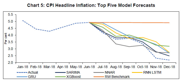
& Light | CPI-exc. Food & Fuel | | Sample Period | 2002–18 | 2012–18 | 2012–18 | 2012–18 | 2012–18 | | Mean | 6.535 | 6.157 | 6.209 | 6.367 | 6.106 | | Median | 5.620 | 5.316 | 5.780 | 5.795 | 5.235 | | Maximum | 13.388 | 11.505 | 16.650 | 11.910 | 10.320 | | Minimum | 1.460 | 1.460 | -1.690 | 2.490 | 3.830 | | Std. Dev. | 2.729 | 2.634 | 4.211 | 2.472 | 1.785 | | Skewness | 0.408 | 0.373 | 0.256 | 0.413 | 0.792 | | Kurtosis | 2.031 | 1.855 | 2.275 | 2.270 | 2.394 | | Observations | 204 | 84 | 84 | 84 | 84 | | Jarque–Bera | 13.633 | 6.536 | 2.758 | 4.254 | 10.067 | | Probability | 0.001 | 0.038 | 0.252 | 0.119 | 0.007 | Chart 2 shows clear shifts in mean inflation over time (it rises till 2010 and then falls). The recent disinflation phase, however, does not show any shift in mean but depicts a moderation in trend inflation (Chart 3). 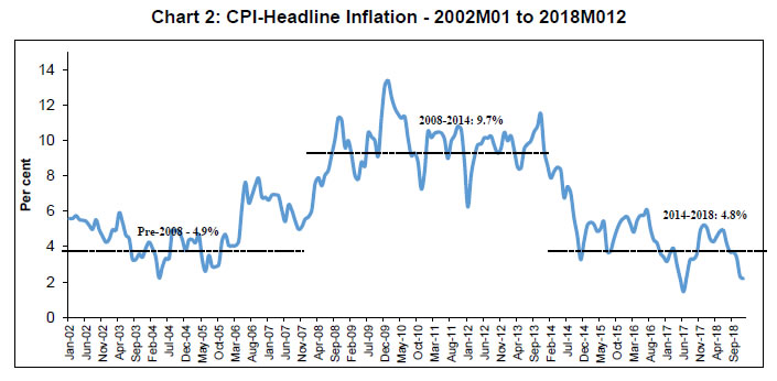 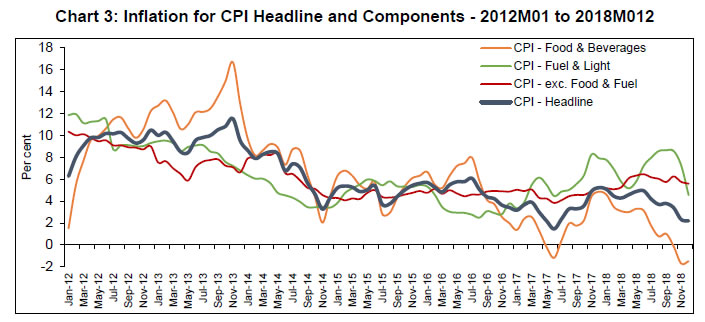 Seasonality in time-series data can manifest in three forms: deterministic, residual, and stochastic. Inflation calculated as the year-on-year (YoY) growth rate of CPI is generally assumed to contain no seasonality but the seasonal adjustment methods7 only control for ‘deterministic seasonality’ in the data. Interestingly, we do find evidence for the presence of seasonality in all four inflation series. We plot both ACF and PACF for headline inflation over longer lag orders and note the significant spikes in PACF at lag orders 12-13, 24-25 and 36-37 pointing towards serial correlation at seasonal frequencies (Chart 4). A plot of cross-correlation between various lags of headline inflation suggests strong serial correlation with seasonal lags. A similar pattern is observed for food, fuel and core inflation series but it is the weakest for fuel inflation. This could, inter alia, be due to ‘residual seasonality’ or the tendency of time series to display a predictable seasonal pattern despite being seasonally adjusted. Such issues have been observed in the case of US GDP growth (Owyang and Shell, 2018) as well as US core consumer price inflation (Peneva and Sadee, 2019). The presence of serial correlation at seasonal frequencies could also be due to ‘stochastic seasonality’ or the presence of seasonal unit roots in the data. When tested for the presence of a seasonal unit root, the evidence was mixed. The Canova–Hansen Test did not find the presence of seasonal unit root, whereas the HEGY Test indicated the presence of seasonal unit roots (Table A1.2, Appendix 1) in the headline (subsample), food, fuel and core inflation. These test results are robust to seasonal adjustment of the underlying CPI series prior to calculation of YoY change. Therefore, we included the generalised SARIMA model in our forecasting exercise. Further, this information on the dynamics of inflation data is also crucial to make an appropriate choice of input variables for ML methods. To capture such dynamics of the data, we use autoregressive lags of the data (up to lag order 24) as input variables in the case of ML methods. 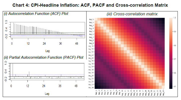 III.4. Estimation/Training Procedure Following the practice in the ML approach of prediction, we divide our sample into two parts: training and test sample. The choice of the train-test split is critical for generating reliable forecasts. The training dataset should be adequate for the model to ‘learn’ from the data and at the same time avoid overfitting. Thus, for each series, we treat the last six months of data as our test sample (Table 2) | Table 2: Train-Test sample for CPI-Headline and Components | | Series | Full Sample | Train | Test | | CPI Headline Inflation | 2002M01 - 2018M12 | 2002M01 - 2018M06 | 2018M07 - 2018M12 | | CPI Food Inflation | 2012M01 - 2018M12 | 2012M01 - 2018M06 | 2018M07 - 2018M12 | | CPI Fuel Inflation | 2012M01 - 2018M12 | 2012M01 - 2018M06 | 2018M07 - 2018M12 | | CPI exc. Food & Fuel Inflation | 2012M01 - 2018M12 | 2012M01 - 2018M06 | 2018M07 - 2018M12 | For deep learning models, input series are transformed (using natural log transformation) and scaled (standard min-max scaling) before they are fed into the model with a view to control the variance of the series. Typically, deep learning models are often used without differencing the series. For non-stationary time series, differencing is one of the most popular approaches. One important aspect of differencing is that while differencing for linear models is a well-suited operation based on formal tests, this is not the case for non-linear models, where the decision for differencing is ad hoc. All models are ‘trained’ or estimated on the training data. An additional consideration during training is related to finding the optimum values of parameters and hyperparameters for each of these models. In ML, the problem of finding the optimum set of hyperparameters for a learning algorithm is called tuning. For all models in our analysis, we use the grid-search method for hyperparameter tuning. Briefly, the grid-search method involves an exhaustive search for optimum values through a manually specified subset space which may include real and/or unbounded values. A grid-search method must be guided by a performance metric, which in our case is Akaike Information Criteria (AIC) for statistical methods and Mean Squared Error (MSE) in the case of ML algorithms. In addition, for each model, we also perform robustness checks and ensure that residuals from the final selected model in each case follow the assumptions of a white noise process (see Chart A1.1 in Appendix 1). III.5. Model Evaluation In order to evaluate the forecasting performance of each model, we rely on the following measures of prediction accuracy, namely Root Mean Square Error (RMSE), relative RMSE and Symmetric Mean Absolute Percentage Error (SMAPE). For headline and subseries inflation, model forecasts are compared for a six-month horizon. IV. Results and Discussion As mentioned earlier, the RW model served as a benchmark for our forecasting exercise. The forecast accuracy of each model over a six-month forecast horizon is presented in Tables 3 to 6. We select top five best performing models for each inflation series based on their SMAPE and present them alongside the actual inflation and RW forecasts. Point forecasts from all models have been provided in Appendix 1. IV.1. Forecasts for Headline, Food, Fuel and Core Inflation We begin our discussion with the forecasts for headline inflation (Table 3). All models barring STL are able to outperform the benchmark RW model. The best forecasting performance is achieved by the SARIMA model of the form (3,1,1)(2,1,1). It is followed by NNAR(15,1,15), deep-learning models (RNN-LSTM and GRU) and XGBoost in terms of forecast accuracy, all able to closely follow the actual inflation path (Chart 5). The parameters, in particular seasonal parameters, of the SARIMA and NNAR model underline important aspects of the DGP discussed in the previous section. Since these models are based on grid-search and minimisation of relevant performance metric, the selection of seasonal AR/MA lags as well as seasonal differencing of order 1 suggests the presence of additional information in the seasonal part of the data. Potential gain in forecast accuracy can be achieved by explicitly including this information in the model. Additionally, all ML models were also able to outperform the ARIMA model by a comfortable margin. | Table 3: Model Accuracy: CPI Headline Inflation (Aggregate) | | Model | RMSE | Relative RMSE | SMAPE | | RW Benchmark | 1.81 | 1.00 | 42.69 | | ARIMA | 1.62 | 0.89 | 39.05 | | SARIMA | 0.24 | 0.13 | 6.88 | | STL | 1.94 | 1.07 | 44.75 | | NNAR | 0.41 | 0.22 | 12.20 | | RNN LSTM | 0.65 | 0.36 | 16.99 | | GRU | 0.63 | 0.35 | 16.77 | | RF | 0.67 | 0.37 | 18.60 | | SVM | 0.74 | 0.41 | 20.09 | | KNN | 0.72 | 0.40 | 17.80 | | XGBoost | 0.62 | 0.34 | 16.90 |
 In the case of food inflation, the SARIMA model again emerges as the best performing model, closely followed by the NNAR model (Table 4). The best model SARIMA(2,1,2)(2,1,1), followed by NNAR(15,1,12), were able to accurately forecast the disinflation and subsequent deflation in food that was seen during the later part of 2018 (Chart 6). RF and XGBoost, which are based on decision-trees, and the KNN model were also close and picked up the food disinflation. The RF, XGBoost and the KNN regression rely on rules based on ‘similarity’ of input data. The strong performance of these models suggests reoccurring patterns in the data that may not be captured in models relying on only very recent observations, such as the ARIMA model. Since these models are adept at handling highly correlated input data, these may be appropriate methods to forecast CPI-food inflation in view of the availability of relevant data such as arrival quantities, wholesale prices and weather indicators. | Table 4: Model Accuracy: CPI-Food & Beverages Inflation | | Model | RMSE | Relative RMSE | SMAPE | | RW Benchmark | 3.41 | 1.00 | 146.94 | | ARIMA | 3.29 | 0.96 | 142.01 | | SARIMA | 0.46 | 0.13 | 65.50 | | STL | 3.75 | 1.10 | 150.51 | | NNAR | 1.47 | 0.43 | 117.09 | | RNN LSTM | 1.72 | 0.50 | 132.03 | | GRU | 4.16 | 1.22 | 159.67 | | RF | 1.38 | 0.40 | 124.87 | | SVM | 4.71 | 1.38 | 159.68 | | KNN | 1.31 | 0.38 | 123.20 | | XGBoost | 1.33 | 0.39 | 125.85 | 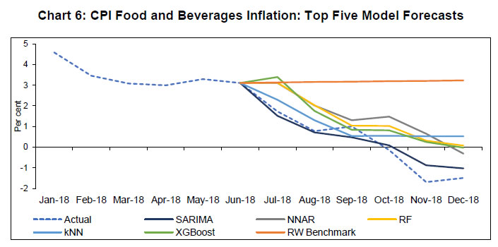 Table 5 provides information on forecast performance for fuel inflation, which depicts a mixed picture. Many ML models, though not all, were able to outperform the benchmark RW forecast and ARIMA forecast. Overall, the forecasts from XGBoost are found to be most precise. NNAR(10,1,7) and RNN-LSTM provided the next best performance in terms of the observed SMAPE. Interestingly, the NNAR model was able to predict the fall in fuel inflation much ahead of other models (Chart 7). In contrast to the headline and food inflation, the SARIMA model in the case of fuel inflation does not rank in the top five models. Recall that the ACF/PACF plots for fuel inflation did not indicate any significant spikes at seasonal frequencies, but the HEGY Test did indicate the presence of seasonal unit root. | Table 5: Model Accuracy: CPI-Fuel and Light Inflation | | Model | RMSE | Relative RMSE | SMAPE | | RW Benchmark | 1.48 | 1.00 | 19.14 | | ARIMA | 1.45 | 0.98 | 16.09 | | SARIMA | 1.32 | 0.89 | 18.05 | | STL | 1.74 | 1.17 | 21.53 | | NNAR | 1.30 | 0.88 | 13.86 | | RNN LSTM | 1.20 | 0.81 | 13.94 | | GRU | 2.11 | 1.42 | 29.66 | | RF | 1.37 | 0.92 | 17.01 | | SVM | 2.04 | 1.37 | 28.32 | | KNN | 1.82 | 1.22 | 23.37 | | XGBoost | 1.08 | 0.73 | 13.20 |
Lastly, in the case of core inflation (or CPI-exc. food and fuel), RW forecasts are quite precise compared to many other statistical/ML methods. It may suggest a complex DGP underlying the data which these models were unable to learn given the short sample. It could also be due to high persistence in core inflation which is captured better by the benchmark RW model. Nevertheless, the SARIMA method was able to generate the best forecasts, yet again underlining its consistency (Chart 8). The chosen SARIMA model is of the form SARIMA (1,1,1)(0,0,1). | Table 6: Model Accuracy: CPI-exc. Food and Fuel Inflation | | Model | RMSE | Relative RMSE | SMAPE | | RW Benchmark | 0.40 | 1.00 | 5.81 | | ARIMA | 0.58 | 1.44 | 8.58 | | SARIMA | 0.20 | 0.51 | 3.26 | | STL | 0.57 | 1.43 | 8.33 | | NNAR | 1.20 | 3.01 | 17.67 | | RNN LSTM | 0.33 | 0.82 | 3.70 | | GRU | 0.35 | 0.88 | 4.27 | | RF | 0.34 | 0.85 | 5.13 | | SVM | 0.44 | 1.11 | 6.97 | | KNN | 0.55 | 1.37 | 6.98 | | XGBoost | 0.40 | 1.01 | 5.13 | 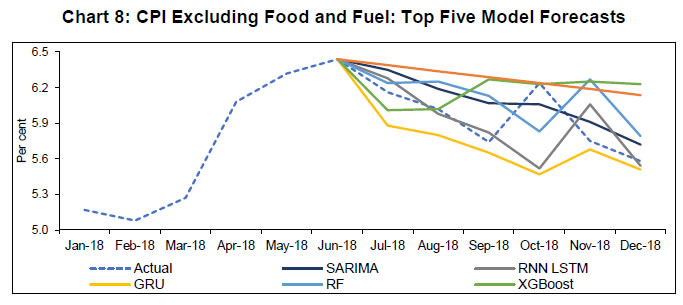 As seen above, the models which incorporate long-term information over the training period provide superior forecasting performance. In the case of ML methods, this is achieved through selection of input variables (autoregressive lags of large order) as well as by construction in the case of deep learning methods. This is also true for the general SARIMA method. The superior forecast performance of such models, especially NNAR and SARIMA, also reflects the presence of the seasonality element in the inflation series. Deterministic seasonality usually denotes constant seasonal means. On the other hand, unit root seasonality captured by the SARIMA model represents seasonal means which evolve over time. Intuitively, this may signify that seasonal patterns repeat themselves but only roughly, as they may be expected to undergo change as the economy evolves. As the inflationary process in India has undergone a structural change during our training period (adoption of the flexible inflation targeting framework and falling fuel and more recently food prices), it could be one of the sources for this time-varying seasonality. Similarly, the forecasting exercise on core inflation also throws some important questions. Compared to the headline inflation forecast, the models with respect to the core inflation appear to feature all the typical improvements one would expect from this core series given its high degree of persistence. Despite this, the SARIMA model was found to forecast this component better. This leads to the following question: Is stochastic seasonality such an endemic feature of the inflationary process that it even influences the core inflation? We repeated the same exercise on core inflation after the seasonal adjustment of the underlying CPI series and found that the SARIMA method still outperformed other methods. This suggests the criticality of implied time-varying seasonality for forecasting exercises. We now turn our attention to some more issues related to inflation forecasting and attempt to provide empirical evidence to this effect. The first of these relates to the performance of forecast combinations. The second question pertains to the approach of directly forecasting headline inflation compared to separately forecasting its components (food, fuel and core) and combine them to arrive at a final forecast for headline inflation. IV.2. Forecast Combinations Combining the forecasts from different ‘competing’ forecasting models is not a new theme in the literature. Bates and Granger (1969), a seminal work in the area of forecast combination, concluded that combining forecasts often leads to better forecasts. A forecast combination is motivated by the fact that any forecast model is at best only an approximation of the true data generating process (DGP), thus more than one model with similar predictive accuracy can be estimated for the same target variable. Forecasts are also state-dependent making them prone to errors related to misspecification, structural breaks and uncertainty related to wider economic changes. In this case, any one model can never be expected to always perform well at all times. Empirically, combination forecasts are argued to work well providing stable performance over time, acting as insurance against model instability (Elliot and Timmerman, 2005). Since Bates and Granger (1969), many other approaches have been suggested in the literature for optimum combination of forecasts. These approaches treat forecast combination as a model selection and constrained parameter estimation problem, suggesting the use of least squares, shrinkage and Bayesian approaches to forecast combination. In fact, many ML models have such techniques inbuilt via bootstrapping, bagging and boosting methods. Some empirical studies have also found that instead of complicated weighing schemes that rely on estimated combination weights, simple equal weighted forecast combination perform well comparatively (Smith and Wallis, 2009). Superior performance of forecast combinations compared to individual models is also one of the results established in the M-competitions. Using our inflation forecasts, we constructed simple forecast combinations based on equal weights given to each model. As an alternative to this simple weighing scheme, we also combined forecasts based on inverse RMSE weights. The accuracy measures for forecast combination based on top five models for each series are given in Table 7. | Table 7: Inflation Forecast Combinations | | Series | Combination Models | Weights | RMSE | SMAPE | | CPI-headline | SARIMA, NNAR, RNN-LSTM, GRU, XGBoost | equal | 0.38 | 10.7 | | Inverse RMSE | 0.51 | 13.89 | | CPI-food | SARIMA, NNAR, RF, KNN, XGBoost | equal | 0.94 | 100.2 | | Inverse RMSE | 1.26 | 121.3 | | CPI-fuel | ARIMA, NNAR, RNN-LSTM, RF, XGBoost | equal | 0.83 | 10.4 | | Inverse RMSE | 1.00 | 12.4 | | CPI-exc. food & fuel | SARIMA, RNN-LSTM, GRU, RF, XGBoost | equal | 0.20 | 2.7 | | Inverse RMSE | 0.25 | 3.5 | It is evident that the simple average forecast combination outperformed all individual models except in the case headline and food, where it is outperformed by the individual SARIMA model. We also computed simple average forecast combinations using various subsets of the top five models, each pointing towards similar results. The inverse RMSE weighted8 forecast combination was not found to perform better than the simple weighing scheme. However, the accuracy gains from forecast combination are visible in terms of overall reduction in RMSE/SMAPE. Given the difficulty in deciding on a single best model, simple average forecast combinations may be considered as a preferred method. Penalising models based on their past performance, such as using weights based on past performance, may result in a loss in forecast accuracy. IV.3. Aggregate vs. Disaggregate Inflation Forecasts The underlying index of CPI-headline is a composite index constructed based on component indices. Therefore, a forecaster may choose to directly forecast headline inflation or separately forecast each component index and then aggregate these forecasts to form the headline forecast. Information from component indices can improve forecast accuracy provided they follow different DGPs, but it can also introduce more noise into the data and, therefore, reduce the accuracy. In this context, Chaudhuri and Bhaduri (2019) find that for Wholesale Price Index (WPI) and its constituents, the forecasting approach based on component indices outperforms the approach to directly forecast WPI inflation. We attempt to address the same question using the data and forecasts of CPI. Using the official weights, we combine the three components – food, fuel and core – to compute the headline inflation forecast for each type of model with the aim to assess the accuracy gains from the ‘disaggregate’ approach relative to the ‘aggregate’ approach for any given model. A comparison of RMSE/SMAPE for any given model indicates that the approach to directly forecasting headline inflation provides better accuracy than the alternative approach (Table 8). In addition, we also construct a forecast for headline inflation based on best performing model for respective component, namely SARIMA for food and core inflation, and XGBoost for fuel inflation (Chart 9). The RMSE and SMAPE for the resultant forecast is 0.68 and 16.68, respectively. Direct forecasts obtained from SARIMA, NNAR and even RF methods are better compared to ‘disaggregate’ inflation forecast. Prima facie these results suggest that there are no apparent gains from forecasting each component individually and then combining them to compute the headline inflation forecast. | Table 8: Forecast Accuracy: Aggregate versus Disaggregate | | Model | Aggregate | Disaggregate | Aggregate | Disaggregate | | | RMSE | RMSE | SMAPE | SMAPE | | RW Forecast | 1.69 | 1.79 | 40.62 | 42.51 | | ARIMA | 0.92 | 0.93 | 24.24 | 23.57 | | SARIMA | 0.29 | 0.64 | 8.40 | 17.29 | | STL | 2.00 | 2.06 | 45.83 | 46.78 | | NNAR | 0.20 | 1.22 | 5.03 | 31.21 | | RNN LSTM | 0.75 | 0.90 | 16.85 | 23.79 | | GRU | 1.66 | 1.81 | 40.08 | 44.31 | | RF | 0.67 | 0.83 | 15.33 | 21.95 | | SVM | 0.75 | 2.29 | 17.79 | 52.51 | | KNN | 0.93 | 0.85 | 22.00 | 19.16 | | XGBoost | 0.73 | 0.83 | 16.61 | 22.09 |
V. Conclusion and the Way Forward The availability of large volume and high-frequency data has allowed researchers to explore more complex models which can capture this data to improve forecasting accuracy. The field of machine learning offers a new paradigm with tools and methods to incorporate this in a policymaker’s forecasting toolkit. In the context of forecasting inflation for India, we review several ML methods and apply them to forecast headline inflation and its components. We restrict ourselves to only univariate time-series space and a short-term forecast horizon of six months. The main findings of this paper are as follows. First, we find that ML methods, especially neural networks and tree-based methods, are able to outperform RW and ARIMA models. Second, in the case of headline and food inflation, the SARIMA method provides overall best forecasts. In fact, SARIMA and XGBoost methods constantly rank amongst the best five models in terms of their accuracy scores. The superior performance of the SARIMA method perhaps points towards the presence of seasonal unit roots and residual seasonality in the data. Third, simple average-based forecast combinations generally outperform all individual models. Simple weight scheme was found to outperform the complex weight method. Notwithstanding the debate on optimum combination method, these results suggest that forecast combination is a good practice to achieve better forecasts. Fourth, in comparing the approaches of directly forecasting headline inflation versus separately forecasting its components and combining them, no meaningful gains were observed from the latter approach. Fifth, our analysis also suggests that accuracy gains can be achieved in economic forecasting by adopting techniques from the ML paradigm such as algorithm-based hyperparameter tuning and train-test validation strategy. Before we conclude, some of the caveats of our forecasting exercise, which may also be generally applicable to ML-based forecasting, need to be mentioned. First, any good forecast must be accompanied by precise confidence intervals to explicitly describe the uncertainty about the forecasts. Confidence intervals in case of statistical methods are based on a well-defined stochastic model. On the other hand, generating a confidence interval is not very straightforward in the case of ML methods. One popular approach to generate confidence intervals around model predicted values relies on iterative bootstrapped sampling of prediction errors either from a normal distribution or historical values. Using this approach, we were able to obtain confidence intervals for the NNAR method; however, a word of caution is needed as this approach is yet to stabilise before it can be used for policy purposes. Second, the generation of out-of-sample forecasts may be sensitive to the sample selection for training/testing of the model. It may, therefore, be appropriate to generate similar forecasts for a different train-test data using rolling or recursive forecasting methods. Third, the forecasting accuracy of ML methods must also be ascertained for different forecast horizons of short (1-3 periods ahead), medium (4-12 periods ahead) and long (more than 12 periods ahead) term. Fourth, ML methods are often termed a ‘black box’ which does not provide any information on how the forecasts are generated. However, methods to derive inference and causal interpretation are an active area of research today, lying at the intersection of computer science and statistics. Nascent literature on using ‘Shapley value’ regression – a concept from game theory to derive statistical inference from ML methods – is gradually emerging (Joseph, 2019). Model agnostic methods, such as Shapley Additive Explanations (SHAP) and Local Interpretable Model-agnostic Explanation (LIME) are techniques being developed to understand the modelled relationship between input-output variables globally as well as locally for each predicted observation or group of observations.
References Ahmed, N. K., Atiya, A. F., Gayar, N. E., and El-Shishiny, H. (2010). An empirical comparison of machine learning models for time series forecasting. Econometric Reviews, 29(5–6), 594–621. Atkeson, A., & Ohanian, L. E. (2001). Are Phillips curves useful for forecasting inflation? Federal Reserve Bank of Minneapolis Quarterly Review, 25(1), 2–11. Ban, T., Zhang, R., Pang, S., Sarrafzadeh, A., & Inoue, D. (2013). Referential knn regression for financial time series forecasting. In International Conference on Neural Information Processing (pp. 601–608). Berlin, Heidelberg: Springer. Bates, J. M., & Granger, C. W. (1969). The combination of forecasts. Journal of the Operational Research Society, 20(4), 451–468. Breiman, L. (2001). Random forests. Machine learning, 45(1), 5–32. Retrieved from: https://link.springer.com/content/pdf/10.1023/A:1010933404324.pdf. Chakraborty, C., & Joseph, A. (2017). Machine learning at central banks (No. 674). Bank of England. Chaudhuri, K., & Bhaduri, S. N. (2019). Inflation Forecast: Just use the Disaggregate or Combine it with the Aggregate. Journal of Quantitative Economics, 1-13. Chung, J., Gulcehre, C., Cho, K., & Bengio, Y. (2015). Gated feedback recurrent neural networks. In International Conference on Machine Learning, vol. 37 (pp. 2067–2075). Chen, T., & Guestrin, C. (2016). Xgboost: A scalable tree boosting system. In Proceedings of the 22nd ACM SIGKDD International Conference on Knowledge Discovery and Data Mining (pp. 785–794). Retrieved from: https://arxiv.org/pdf/1603.02754.pdf. Cleveland, R. B., Cleveland, W. S., McRae, J. E., & Terpenning, I. (1990). STL: A seasonal-trend decomposition. Journal of Official Statistics, 6(1), 3–73. Cook, T., & Smalter Hall, A. (2017). Macroeconomic indicator forecasting with deep neural networks. Federal Reserve Bank of Kansas City, Research Working Paper (17–11). Diebold, F. X. (1998). The past, present, and future of macroeconomic forecasting. Journal of Economic Perspectives, 12(2), 175–192. Elliott, G., & Timmermann, A. (2005). Optimal forecast combination under regime switching. International Economic Review, 46(4), 1081–1102. Garcia, M. G., Medeiros, M. C., & Vasconcelos, G. F. (2017). Real-time inflation forecasting with high-dimensional models: The case of Brazil. International Journal of Forecasting, 33(3), 679–693. Goodfellow, I., Bengio, Y., & Courville, A. (2016). Deep Learning. MIT Press. https://www.deeplearningbook.org/. Härdle, W., & Vieu, P. (1992). Kernel regression smoothing of time series. Journal of Time Series Analysis, 13(3), 209–232. Hochreiter, S., & Schmidhuber, J. (1997). Long short-term memory. Neural computation, 9(8), 1735–1780. Hyndman, R., & Khandakar, Y. (2008). Automatic time series forecasting: The forecast package for R. Journal of Statistical Software, 27(3), 1–22. doi:http://dx.doi.org/10.18637/jss.v027.i03. Hyndman, R. J., & Athanasopoulos, G. (2018) Forecasting: principles and practice (2nd ed.), Melbourne: OTexts:. Joseph, A. (2019). Shapley regressions: A framework for statistical inference on machine learning models. Bank of England Staff Working Paper 784. Liaw, A., & Wiener, M. (2002). Classification and regression by random Forest. R news, 2(3), 18–22. Makridakis, S., & Hibon, M. (2000). The M3-Competition: Results, conclusions and implications. International Journal of Forecasting, 16(4), 451–476. Makridakis, S., Spiliotis, E., & Assimakopoulos, V. (2018a). Statistical and Machine Learning forecasting methods: Concerns and ways forward. PloS one, 13(3), e0194889. — (2018b). The M4 Competition: Results, findings, conclusion and way forward. International Journal of Forecasting, 34(4), 802–808. Malhotra, A., & Maloo, M. (2017). Understanding food inflation in India: A machine learning approach. Retrieved from: https://arxiv.org/ftp/arxiv/papers/1701/1701.08789.pdf. McAdam, P., & McNelis, P. (2005). Forecasting inflation with thick models and neural networks. Economic Modelling, 22(5), 848–867. Medeiros, M. C., Vasconcelos, G. F., Veiga, Á., & Zilberman, E. (2019). Forecasting Inflation in a data-rich environment: the benefits of machine learning methods. Journal of Business & Economic Statistics, 1-45. Mullainathan, S., & Spiess, J. (2017). Machine learning: An applied econometric approach. Journal of Economic Perspectives, 31(2), 87–106. Nakamura, E. (2005). Inflation forecasting using a neural network. Economics Letters, 86(3), 373–378. Owyang, M. T., & Shell, H. (2018). Dealing with the leftovers: Residual seasonality in GDP. The Regional Economist, 26(4). Peneva, E. V., & Sadee, N. (2019). Residual seasonality in core consumer price inflation: An update (No. 2019-02-12). Board of Governors of the Federal Reserve System (US). Pescatori, A., & Zaman, S. (2011). Macroeconomic models, forecasting, and policymaking. Economic Commentary, 2011-19, 5 October. Pradhan, R. P. (2011). Forecasting inflation in India: An application of ANN Model. International Journal of Asian Business and Information Management (IJABIM), 2(2), 64–73. Rani, S. J., Haragopal, V. V., & Reddy, M. K. (2017). Forecasting inflation rate of India using neural networks. International Journal of Computer Applications, 158(5), 45–48. RBI. (2014). Report of the Expert Committee to Revise and Strengthen the Monetary Policy Framework (Chairman: Urjit R. Patel), Reserve Bank of India, Rumelhart, D. E., Hinton, G. E., & Williams, R. J. (1988). Learning representations by back-propagating errors. Cognitive modeling, 5(3), 1. Sanyal, A., & Roy, I. (2014). Forecasting major macroeconomic variables in India: Performance comparison of linear, non-linear models and forecast combinations. RBI Working Paper Series No. 11/2014. Smith, J., & Wallis, K. F. (2009). A simple explanation of the forecast combination puzzle. Oxford Bulletin of Economics and Statistics, 71(3), 331–355. The Economist (2017). The world’s most valuable resource is no longer oil, but data. The Economist: New York, NY, USA. Retrieved from: https://www.economist.com/leaders/2017/05/06/the-worlds-most-valuable-resource-is-no-longer-oil-but-data. Ülke, V., Sahin, A., & Subasi, A. (2018). A comparison of time series and machine learning models for inflation forecasting: Empirical evidence from the USA. Neural Computing and Applications, 30(5), 1519–1527. Varian, H. R. (2014). Big data: New tricks for econometrics. Journal of Economic Perspectives, 28(2), 3–28. Zhang, G. P. (2007). Avoiding pitfalls in neural network research. IEEE Transactions on Systems, Man, and Cybernetics, Part C (Applications and Reviews), 37(1), 3–16.
Appendix 1: Statistical Tests and Model Forecasts | Table A1.1: Unit Root Tests | | Series | ADF Test
(null: data is non-stationary) | KPSS Test
(null: data is stationary) | | In Levels | stat | p-value | stat | p-value | | CPI - headline | -1.301 | 0.869 | 0.850 | 0.010 | | CPI - food & beverages | -3.118 | 0.117 | 1.600 | 0.010 | | CPI - fuel & light | -2.293 | 0.456 | 0.921 | 0.010 | | CPI - exc. food & fuel | -1.795 | 0.660 | -6.215 | 0.753 | | First Difference | stat | p-value | stat | p-value | | CPI - headline | -6.501 | 0.010 | 0.141 | 0.100 | | CPI - food & beverages | -4.483 | 0.010 | 0.257 | 0.100 | | CPI - fuel & light | -5.038 | 0.010 | 0.148 | 0.100 | | CPI - excl. food & fuel | -4.941 | 0.010 | 0.277 | 0.100 |
| Table A1.2: Number of Seasonal Differences Based on Seasonal Unit Root Tests | | | Canova-Hansen Test | HEGY Test | | Series | (p < 0.05) | (p < 0.05) | | CPI - headline | 0 | 0 | | CPI - headline | 0 | 1 | | CPI - food & beverages | 0 | 1 | | CPI - fuel & light | 0 | 1 | | CPI - exc. food & fuel | 0 | 1 |
| Table A1.3: Model Forecasts: CPI Headline Inflation (Aggregate) | | | Jul-18 | Aug-18 | Sep-18 | Oct-18 | Nov-18 | Dec-18 | | Actual | 4.17 | 3.69 | 3.77 | 3.38 | 2.33 | 2.19 | | Statistical/Decomposition | | RW Forecast | 4.92 | 4.92 | 4.91 | 4.91 | 4.91 | 4.90 | | ARIMA | 4.84 | 4.77 | 4.72 | 4.69 | 4.67 | 4.65 | | SARIMA (R) | 4.45 | 4.03 | 4.03 | 3.89 | 3.29 | 3.14 | | SARIMA (Python) | 4.25 | 3.80 | 3.82 | 3.51 | 2.80 | 2.49 | | STL | 4.99 | 5.05 | 4.96 | 4.96 | 5.08 | 5.10 | | Machine Learning | | NNAR (R) | 4.35 | 3.36 | 3.16 | 3.26 | 2.76 | 2.71 | | NNAR (Python) | 4.77 | 4.13 | 3.72 | 3.79 | 3.45 | 2.55 | | RNN LSTM | 4.79 | 4.16 | 3.77 | 3.83 | 3.52 | 2.75 | | GRU | 4.90 | 4.38 | 3.89 | 3.67 | 3.32 | 2.70 | | RF | 4.81 | 4.23 | 3.83 | 3.90 | 3.25 | 3.11 | | SVM | 5.11 | 4.09 | 4.04 | 3.95 | 2.99 | 3.37 | | KNN | 5.00 | 3.91 | 3.81 | 3.72 | 3.63 | 2.92 | | XGBoost | 4.58 | 3.91 | 4.01 | 3.70 | 3.27 | 3.19 |
| Table A1.4: Model Forecasts: CPI Food Inflation | | | Jul-18 | Aug-18 | Sep-18 | Oct-18 | Nov-18 | Dec-18 | | Actual | 1.73 | 0.78 | 1.01 | -0.14 | -1.69 | -1.49 | | Statistical/Decomposition | | RW Forecast | 3.13 | 3.15 | 3.17 | 3.19 | 3.21 | 3.23 | | ARIMA | 1.16 | 0.83 | 1.77 | 1.53 | 0.24 | 0.13 | | SARIMA (R) | 1.16 | 0.83 | 1.70 | 1.50 | 0.23 | 0.12 | | SARIMA (Python) | 1.52 | 0.71 | 0.48 | 0.09 | -0.88 | -1.03 | | STL | 3.58 | 3.60 | 3.23 | 3.30 | 3.65 | 3.80 | | Machine Learning | | NNAR (R) | 2.55 | 1.64 | 0.92 | 0.65 | 0.81 | 0.74 | | NNAR (Python) | 3.11 | 2.02 | 1.31 | 1.48 | 0.65 | -0.31 | | RNN LSTM | 3.07 | 2.15 | 1.56 | 1.70 | 1.03 | 0.24 | | GRU | 4.84 | 4.31 | 4.35 | 4.16 | 3.55 | 3.48 | | RF | 3.12 | 2.03 | 1.04 | 1.03 | 0.32 | 0.08 | | SVM | 4.71 | 4.38 | 4.45 | 4.76 | 4.53 | 4.59 | | KNN | 2.29 | 1.31 | 0.54 | 0.55 | 0.53 | 0.53 | | XGBoost | 3.39 | 1.76 | 0.84 | 0.81 | 0.25 | -0.02 |
| Table A1.5: Model Forecasts: CPI Fuel Inflation | | | Jul-18 | Aug-18 | Sep-18 | Oct-18 | Nov-18 | Dec-18 | | Actual | 7.96 | 8.55 | 8.63 | 8.55 | 7.24 | 4.54 | | Statistical/Decomposition | | RW Forecast | 7.16 | 7.10 | 7.04 | 6.98 | 6.92 | 6.86 | | ARIMA | 7.55 | 7.62 | 7.64 | 7.65 | 7.65 | 7.65 | | SARIMA R | 7.40 | 7.44 | 7.11 | 6.78 | 5.82 | 5.72 | | SARIMA Python | 7.05 | 7.04 | 6.93 | 6.58 | 6.08 | 6.57 | | STL | 6.87 | 6.85 | 6.93 | 6.98 | 7.33 | 7.48 | | Machine Learning | | NNAR (R) | 8.32 | 8.38 | 7.84 | 6.45 | 5.02 | 4.41 | | NNAR (Python) | 7.01 | 7.77 | 8.41 | 8.50 | 8.41 | 7.03 | | RNN LSTM | 6.85 | 7.76 | 8.41 | 8.48 | 8.40 | 6.86 | | GRU | 5.78 | 6.01 | 6.24 | 6.29 | 6.41 | 6.57 | | RF | 6.78 | 7.39 | 7.83 | 8.15 | 8.18 | 7.16 | | SVM | 6.18 | 6.01 | 6.06 | 6.18 | 6.19 | 5.96 | | KNN | 5.64 | 6.30 | 7.37 | 7.37 | 7.37 | 7.06 | | XGBoost | 6.68 | 7.67 | 8.54 | 8.38 | 8.35 | 6.37 |
| Table A1.6: Model Forecasts: CPI Excluding Food and Fuel Inflation | | | Jul-18 | Aug-18 | Sep-18 | Oct-18 | Nov-18 | Dec-18 | | Actual | 6.16 | 6.02 | 5.74 | 6.24 | 5.75 | 5.58 | | Statistical/Decomposition | | RW Forecast | 6.39 | 6.34 | 6.29 | 6.24 | 6.19 | 6.14 | | ARIMA | 6.44 | 6.44 | 6.44 | 6.44 | 6.44 | 6.44 | | SARIMA (R) | 6.35 | 6.19 | 6.07 | 6.06 | 5.91 | 5.72 | | SARIMA (Python) | 6.15 | 5.89 | 5.58 | 5.44 | 5.07 | 4.86 | | STL | 6.38 | 6.41 | 6.43 | 6.43 | 6.43 | 6.47 | | Machine Learning | | NNAR (R) | 6.85 | 6.86 | 7.19 | 7.07 | 7.13 | 7.25 | | NNAR (Python) | 7.01 | 7.77 | 8.41 | 8.50 | 8.41 | 7.03 | | RNN LSTM | 6.28 | 5.98 | 5.82 | 5.52 | 6.06 | 5.54 | | GRU | 5.88 | 5.80 | 5.65 | 5.47 | 5.68 | 5.51 | | RF | 6.24 | 6.25 | 6.13 | 5.83 | 6.27 | 5.79 | | SVM | 6.61 | 6.47 | 6.35 | 5.88 | 6.22 | 5.79 | | KNN | 6.19 | 5.83 | 5.83 | 5.27 | 6.10 | 6.41 | | XGBoost | 6.01 | 6.02 | 6.27 | 6.23 | 6.25 | 6.23 |
| Table A1.7: Model Forecasts: Disaggregated CPI Headline | | | Jul-18 | Aug-18 | Sep-18 | Oct-18 | Nov-18 | Dec-18 | | Actual | 4.17 | 3.69 | 3.77 | 3.38 | 2.33 | 2.19 | | Statistical/Decomposition | | RW Forecast | 4.95 | 4.93 | 4.91 | 4.89 | 4.87 | 4.86 | | ARIMA | 4.82 | 5.03 | 5.32 | 5.27 | 5.01 | 5.03 | | SARIMA (R) | 4.04 | 3.82 | 4.14 | 4.02 | 3.30 | 3.15 | | SARIMA (Python) | 4.09 | 3.59 | 3.33 | 3.06 | 2.41 | 2.28 | | STL | 5.13 | 5.15 | 5.00 | 5.03 | 5.22 | 5.31 | | Machine Learning | | NNAR (R) | 4.98 | 4.57 | 4.36 | 4.08 | 4.09 | 4.07 | | NNAR (Python) | 5.22 | 5.13 | 5.15 | 5.28 | 4.85 | 3.66 | | RNN LSTM | 4.85 | 4.35 | 4.04 | 3.97 | 3.91 | 3.20 | | GRU | 5.40 | 5.13 | 5.09 | 4.93 | 4.75 | 4.65 | | RF | 4.85 | 4.39 | 3.91 | 3.79 | 3.67 | 3.27 | | SVM | 5.71 | 5.48 | 5.46 | 5.39 | 5.44 | 5.25 | | KNN | 4.36 | 3.79 | 3.51 | 3.25 | 3.63 | 3.76 | | XGBoost | 4.85 | 4.18 | 3.94 | 3.89 | 3.64 | 3.37 |
Appendix 2: Forecasting Models 1. Statistical/Decomposition-based Models Random Walk (RW) According to the RW model, the best possible forecast of a variable is its last observed value. A RW model with a ‘drift’ can be described as: RW (naïve) model is often used as a benchmark model for forecast evaluation exercises. It has also been noted in the literature that it is difficult to beat simple benchmark models such as the RW model (Atkeson and Ohanian, 2001). Therefore, we choose the RW model as a benchmark against which all other models are evaluated. ARIMA ARIMA or autoregressive integrated moving average model combines autoregressive and moving average models. It is one of the most popular forecasting methods for univariate time-series forecasting. It can be represented as: Seasonal ARIMA (SARIMA10) The ARIMA model does not support seasonal data. It expects the input data to be either non-seasonal or seasonally adjusted. However, such adjustment can lead to loss of information leading to forecast errors, especially in the case of stochastic seasonality in the data. The SARIMA model is a more general form of the ARIMA model that explicitly supports univariate time-series data with a seasonal component. It adds three new hyperparameters to model the seasonal component of the data. A model of this type is of the form SARIMA(p,d,q)(P,D,Q)m where (p,d,q) is the order of the AR, integration and MA part of the non-seasonal component of the data, (P,D,Q) is the order of the AR, integration and MA part of the seasonal component and m is the seasonal frequency (e.g. m = 12 for monthly data; 4 for quarterly data). It can be expressed as follows: STL Decomposition STL or the ‘Seasonal and Trend Decomposition with Loess’ is a versatile and robust method for decomposing a time series into its trend, seasonal and remainder components. Loess is a method for estimating non-linear relationships. Originally developed by Cleveland et al. (1990), the STL model decomposes a time series in the following form: 2. ML Algorithms For ML algorithms, we consider a forecast approach where inflation h period-ahead is modelled as a function of input variables measured at time t, i.e. Decision Trees, Bagging and Boosting In its ML application, a decision (also called a regression) tree is a non-parametric model that relies on recursive binary partitioning of the covariate space. Usually displayed in a graph which has the format of a binary decision tree with split nodes and terminal nodes (also called leaves), and which grows from the root node to the terminal nodes. The left panel in Chart A2.2 shows this binary partitioning of target variable space in the case of two features. The graph form of a binary tree with split and terminal nodes for the same is shown in the right panel of Chart A2.2. Regression trees, however, by themselves are found to be weak learners or weak predictors of data as they are prone to the problem of overfitting. To overcome this, many solutions have been proposed which are usually based on ‘bagging’ or ‘boosting’ principles. The idea is to have many independent tree models which jointly outperform any single tree model. Random Forest (RF) Algorithm: Originally proposed by Breiman (2001), the RF algorithm reduces the variance of such regression trees and is based on bagging11 or the bootstrapped12 aggregation of predictions from randomly constructed trees. Therefore, the RF algorithm achieves this by, first, growing an ensemble of decision trees; second, using a randomised sample (with replacement) of input data as well as a random subset of predictor variables to grow n individual regression trees; third, by testing prediction accuracy on the out-of-bag (OOB) data, i.e. data left out from the initial sample; and, fourth, by averaging out all the final predictions to minimise prediction error. Formally, each tree in a random forest is built using the following steps where T represents the entire forest, t represents a single tree, for t = 1 to T: -
Create a bootstrap sample with replacement, S from the training set comprising X, Y and label these Xa, Ya; -
train the tree ft on Xa, Ya; and -
average the predictions to arrive at a final prediction. In a regression problem, predictions for the test instances are made by taking the mean of the predictions made by all trees. This can be represented as follows: Readers can refer to Liaw and Wiener (2002) for an excellent summary of the workings of an RF algorithm. Random forests can deal with very large numbers of explanatory variables, and the proposed model is highly non-linear. Extreme Gradient Boosting (XGBoost) Algorithm: Developed by Chen and Guestrin (2016), XGBoost has been one of the best performing models at international forecasting competitions. Akin to the RF algorithm, an XGBoost model is also a decision tree-based technique. It is also an ensemble learning method offering a systematic solution to combine the predictive power of multiple learners, when relying on single models may not be advisable. The resultant is a single model which gives the aggregated output from several models. XGBoost uses boosting, where decision trees are built sequentially (rather than simultaneously as in the case of random forests) such that each subsequent tree aims to reduce the errors of the previous tree. Each tree learns from its predecessors and updates the residual errors. Hence, the tree that grows next in the sequence will learn from an updated version of the residuals. The objective function of XGBoost at iteration t that needs to be minimised is given by: 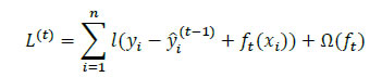 Which can be simplified using a second-order Taylor approximation to the following form, where gi and hi are the first and second order gradients of the loss function: Being at iteration t, the next step would be to build a tree learner that achieves the maximum possible reduction of loss, which in turn is built iteratively through the exact greedy algorithm13. Inbuilt within the XGBoost algorithm is the usage of a gradient descent algorithm to train the model and minimise the error in prediction. Gradient descent is a first-order iterative optimisation algorithm for finding the minimum of a function. To find the local minima of a function using this approach, steps proportional to the negative of the gradient of the function are taken at the current point (Chart A2.3). The steps are in turn controlled using the learning rate which decides the speed and accuracy with which optimum solutions are found. Artificial Neural Network (ANN) and Deep Learning14 models A neural network (NN) model can be depicted as a set of ‘neurons’ which are organised in the form of layers. The building block of a NN is a perceptron shown in Chart A2.4 which can be represented as, The most basic NN model has three distinct set of layers: one, an input layer representing inputs of the model; second, a hidden layer representing a set of functional nodes; and, third, an output layer representing the output of the model. The presence of the hidden layer lends non-linearity to the NN model, without which an NN model is akin to a linear regression model. In the equation above x(k) is a vector of input representing the input layer and ω is a corresponding vector of weights. In the hidden layer, an input-weight combination is transformed via a non-linear function F{.}, such as a sigmoid function, to be passed on to the next layer. The next layer could be another hidden layer or the output layer. For instance, inputs into a hidden node j in are combined linearly as: while the input can be then transformed using a non-linear sigmoid function as: Neural Network Autoregression (NNAR) Model The feed forward fully connected type of network is a type of NN architecture which can consist of several hidden layers of computational nodes stacked between an input and an output layer (Chart A2.5). Since the data only move in one direction through the network, the model is feed forward in nature. Likewise, the network is fully connected, as output of each node in a hidden layer feeds into each of the nodes in the following layer as an input. 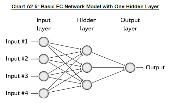 Such a network can be compared to a linear autoregressive model, in the sense that lagged values of a time-series variable are used as an input into the model. Thus, some practitioners often term this model as a neural network autoregression (NNAR) model15. An NNAR model using last p observations as an input is comparable to an ARIMA(p,0,0) model but without the assumption of linear parameters. Additionally, to capture seasonal data, the model can be fed with lagged seasonal terms as inputs, i.e. values observed at the same time in the previous year. The presence of the hidden layer allows for non-linear mapping between input and output of the model. We consider a model of the form NNAR (p, P, k) where p indicates the number of autoregressive lags, P indicates the number of seasonal autoregressive lags and k indicates the number of nodes in the hidden layer. We consider only one hidden layer. In training the model, the weights start with random values which are then updated by learning from the observed data. The model is trained several times (each time a model is trained is called an epoch) using different randomised initial values for weights. The final prediction is made by averaging the predictions across all epochs. Recurrent Neural Network – Long Short-term Memory (RNN-LSTM) Network Traditional ANNs, such as the one described earlier, assume that all inputs are independent of each other. This assumption breaks down in the case of sequential data. The RNN models (Rumelhart et al., 1988) which were developed during the application of neural networks to language parsing, speech recognition and translation, are suitable when the data has a sequential structure or temporal structure. Since this type of model can capture the sequence in which input data is fed into them, they are extremely suitable for modelling time-series data. We focus on the long short-term memory (LSTM) type network first suggested by Hochreiter and Schmidhuber (1997). It draws on the broad contextual features of the model (long-run memory) as well as the information provided by the recent inputs of the sequence (short-run memory). A nice explanation of the LSTM architecture is provided by Hall and Cook (2017), which is depicted in Chart A2.6. Each Input xi is fed into a computational node that also accepts inputs from the output of the preceding layer (denoted si,hi). The term si represents the state of the network at the ith member of the sequence - the long running memory for the sequence, as given by the elements of the sequence to which the network has been exposed. The term hi is the output of the layer that corresponds to a given element i in the sequence. This architecture can thus be understood as consisting of many layers and having the following properties: each layer corresponds to a particular input element in the sequence; each layer receives the network's long-run understanding of the previous sequence; and each layer receives the output generated from the previous element in the sequence. 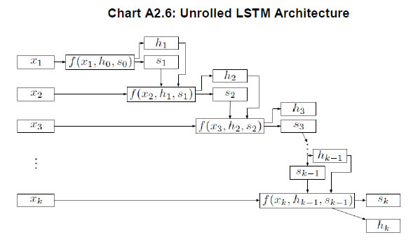 Another way to visualise an RNN-LSTM architecture would be to look at its ‘rolled’ version (Chart A2.7). The ‘rolled’ version of a recurrent (LSTM) architecture represents the architecture as a ‘cell’. The arrow from the cell to itself indicates the feedback loop created as the output from one element of the sequence taken as input along with the next element in the sequence. 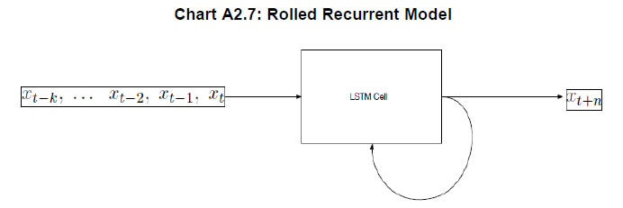 The backpropagation through time (BPTT) algorithm is used to train the RNN model, i.e. find the optimal weights for the network. The RNN is shown one input at each time step to predict one output. BPTT unrolls all input time steps, with each time step having one input time step, one copy of the network, and one output. Prediction errors are then calculated and collected for each time step. The network is then rolled back to update the weights. We can summarise the algorithm as follows: (i) present a sequence of time steps of input and output pairs to the network; (ii) unroll the network, then calculate and accumulate errors across each time step; (iii) roll-up the network and update weights; (iv) repeat. However, BPTT can be computationally expensive as the number of time steps increases. The final architecture of the model can be summarised by the following set of equations: 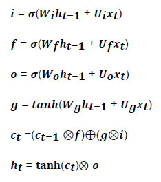 Here ‘i’,’f’ and ‘o’ are the input, forget and output gates. They are computed using the same equations but with different parameter matrices. The sigmoid function restricts the output of these gates between 0 and 1, so the output vector produced can be multiplied element-wise with another vector to define how much of the second vector can pass through the first one. The forget gate controls for how much of the previous state h(t-1) one wants to allow to pass through. The input gate defines how much of the newly computed state for the current input x(t) is to be let through, and the output gate is defined by how much of the internal state is to be exposed to the next layer. The internal hidden state ‘g’ is computed based on the current input x(t) and the previous hidden state h(t-1). Given ‘i’, ‘f’, ‘o’ and ‘g’, one can now easily calculate the cell state C(t) at time t in terms of C(t-1) at time t-1 multiplied by the forget gate and the state ‘g’ multiplied by the input gate ‘i’. This basically represents an approach to combine the previous memory and the new input. Setting the forget gate to ‘o’ ignores the old memory and setting the input gate to ‘o’ ignores the newly computed state. Finally, the hidden state h(t) at time t is computed by multiplying the memory C(t) with the output gate. Gated Recurrent Unit (GRU) Network Over the past few years, the Gated Recurrent Unit or GRU has also emerged as an effective new tool for modelling sequential data (Chung et al., 2015). They have fewer parameters than LSTM but often deliver similar or better performance. Just like the LSTM, the GRU controls the flow of information, but without the use of a typical memory unit. Instead of using a separate cell state, the GRU uses the hidden state as memory. The following Chart A2.8 shows the topology of a GRU memory block (node). 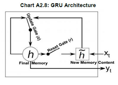 It contains an update gate (z) and reset gate (r). The reset gate determines how to combine the new input with previous memory. On the other hand, the update gate defines how much of the previous memory to use in the present. Together these gates give the model the ability to explicitly save information over many time steps. The GRU is designed to adoptively reset or update its memory content. The GRU is also trained using BPTT. The final architecture of the model can be summarised by the following set of equations: k-Nearest Neighbours (KNN) Regression One of the simplest and best-known non-parametric algorithms is the k-nearest neighbours regression. In this method, an observation is modelled as its k nearest observations in the feature space, such that for a regression problem, an observation is assigned to the mean value of its nearest neighbours, where weights may be applied. Ban et al. (2013) describe the intuition behind the application of this approach to univariate time series: “consistent data-generating processes often produce observations of repeated patterns of behavior. Therefore, if a previous pattern can be identified as similar to the current behavior of the time series, the subsequent behavior of previous pattern can provide valuable information to predict the behavior in the immediate future.” In other words, this task requires ranking historic events in terms of ‘similarity’ (these are usually referred to as fitting or learning events). Then each an event is assigned to a class to which a majority of these observations belong. Hence, KNN is completely non-parametric – no assumptions are made about the shape of the decision boundary. In order to determine ‘similarity’, a metric of distance is required in addition to a specific value of k that minimises prediction error. Various metrics have been used in order to measure distance in the multidimensional space, including Euclidian distance (Härdle and Vieu, 1992). The algorithm works as follows. It computes the Euclidean distance from the input data to the target data. Given a value for k and a prediction point xi, KNN regression then identifies the k observations that are closest to xi, represented by N0. It orders each observation in the training sample in the increasing order of distance. An optimal number k of nearest neighbours is found based on a validation technique such as cross-validation. Finally, it calculates an inverse distance weighted average with the k-nearest multivariate neighbours to estimate F(xi) using the average of all the responses in . In other words: An example of a KNN regression model fitting on training data is provided in Chart A2.9. The black straight line shows the true model while the blue line is the model fitted by KNN regression when k equals 1 (left panel) and k equals (5). A smoother model fit reflecting the true model is obtained as k moves close to its optimum value. Support Vector Machine (SVM) Regression In many situations, the data may not be linearly separable making it difficult to model via a line or a hyperplane. In addition, the exact position of this separation boundary might also not be known. To solve the first issue, the data can be projected into other dimension(s) such that the data is linearly separable given the projection is chosen aptly. The second issue can be solved by fixing a way to identify the best separation line. Intuitively, these solutions are a major part of the SVM algorithm (Chart A2.10). After projection of data into a new feature space, the SVM algorithm defines the best line as the one which has the maximum vertical distance to its closest observations. These closest data points are called support vectors from which the algorithm derives its name. Consider the linear case to find f(x) with the minimal norm value which can be formulated as an optimisation problem as follows: where C is a positive numeric value to control the penalty on observations that lie outside the margin and prevents overfitting determining the smoothness of f(x) and the deviations from the margin. Likewise, the same algorithm can be extended to regression problems in the general case of non-linear separation boundary. The SVM is an extension of the support vector machine classifier that results from enlarging the feature space in a specific way, using kernels, in order to accommodate a non-linear boundary between the observations. A kernel is a function that quantifies the similarity of two observations. In its general form, it can be shown as follows:
|