Press Release RBI Working Paper Series No. 03 Does Financial Cycle Exist in India? @Harendra Behera, Saurabh Sharma Abstract #The paper tries to identify the existence of financial cycle in India by examining its main characteristics. Using three distinct methods – turning point analysis, spectral analysis and band-pass filter – and quarterly data on credit, equity prices, house prices and real exchange rate for the period 1960:Q1 through 2018:Q4, the cyclical properties of individual variables are analysed. The individual cycles are combined using principal component analysis to obtain an aggregate measure of financial cycle for India. The overall analysis suggests that there is a well-defined financial cycle in India and the expansionary phases of financial cycle, particularly the peak, provide an early warning signal about rising stress in the banking sector and weakening of economic activity in future. We find that the length and duration of cycles in financial variables are much greater as compared to the business cycle. Further, the evidence suggests that the dominance of medium-term cycles in overall variation of financial variables has increased since mid-1990s coinciding with the rise in the pace of financial liberalisation. While both credit and equity prices drive financial cycles in India, the contribution of house prices has increased since mid-2000s. JEL Classification: C22, E30, E44, E58, G18 Keywords: Financial cycle, business cycle, recession, macro-prudential policy. I. Introduction India’s financial sector has witnessed a large overhang of balance sheet stress with gross non-performing assets of banks increasing from 2.3 per cent of total advances in 2007-08 to 11.2 per cent in 2017-18. A few non-banking financial companies have also started defaulting on their loan repayments since August 2018. During the same period, economic activity in India has been subdued with GDP growth slowing down from 7.7 per cent to 6.8 per cent. The co-existence of financial sector stress along with economic slowdown reminds us the ongoing global debate on financial cycle. The relevance of financial cycle analysis has increased in the post global financial crisis (GFC) period to explain macro-financial dynamics (Borio, 2012) and to predict systemic banking crises (Drehman, et al. 2012; Schuller, et al. 2017). In fact, the ‘lost decade’ of Japan and other financial crises in emerging market economies during mid-1990s were preceded by either prolonged credit booms or asset price booms. These developments have drawn the attention of researchers to explore the relationship between financial variables and business cycle fluctuations. Studies have found a deeper recession when the downturn of financial cycle is associated with that of the business cycle (Claessens et al., 2012; Drehmann et al., 2012). Consequently, central banks, mainly in the advanced countries, have started using financial cycle as a basis for countercyclical macroprudential policies to tame the amplifying effects of financial disruptions on the overall economy. Deciphering the financial cycle is critical in policymaking for several reasons. First, economic crises like the GFC highlighted the negative spillovers of financial sector turbulence on the real economy. Economic theory suggests that “wealth effect” and “change in expectations” are the two broad channels that connect these two segments. Second, from the viewpoint of financial stability, it is very much possible that monetary policy, used mainly for stabilising short-term business cycles, may result in build-up of stress in the financial sector. For example, India had seen a period of benign inflation just before the 2008 crisis. This could have motivated the monetary policy rate to be kept accommodative. The easy monetary policy, may have assisted, if not contributed to the over exuberant credit growth, leading to a rise in non-performing assets in the subsequent years. In this context, measurement of financial cycle becomes useful when it is critical to be selective and manage risk actively. Third, it is found in the literature that financial cycles predict recessions much in advance and thus monitoring the cycles help in smoothening their effects through appropriate policy responses. Contemporary studies in other countries have indicated that a financial cycle is typically longer and has a larger amplitude than the business cycle. If this is true for India, then financial cycle can be a better metric of guidance for countercyclical macro-prudential measures aiming at long-term financial stability. Given the above context, it is important to study financial cycle so as to help in framing suitable policies and to improve the resilience of the financial system. In this paper, we attempt to measure and study the characteristics of financial cycle in India. We have followed a three-step approach to analyse financial cycle. In the first step, we employ turning point analysis and spectral analysis on individual financial variables to get prima facie evidence on underlying financial cycles. Spectral analysis has a peculiar advantage that no a priori assumption is needed to derive the duration and amplitude of the cycle. After confirming the evidence from the first step, we extract financial cycles using frequency domain based asymmetric band-pass filter method. In the third step, the extracted cycles of select financial variables are combined using principal component analysis (PCA) to obtain an aggregate measure of financial cycle. The rest of the paper is organised into five sections. The following section is devoted to literature review. Data and methodology are discussed in Section III and Section IV, respectively. Section V deliberates upon the empirical analysis on financial cycles and the last section provides concluding observations along with policy implications. II. Literature Review The concept and definition of business cycle are well-known while that of financial cycle are still evolving. Business cycle can be described as the rise and fall in aggregate economic activity over a period of time and can be measured using real GDP data. Financial cycle, on the other hand, maps out the expansions and contractions in the financial activities. So far, there is no consensus on the definition of a financial cycle. As Borio (2012) defines, financial cycle can be best thought as “the self-reinforcing interactions between perceptions of value and risk, attitudes towards risk, and financing constraints, which translate into booms followed by busts”. These interactions can magnify economic fluctuations and possibly lead to serious financial distress. The financial cycle is not observed directly. Instead it is extracted from appropriate macro-financial variables such as credit, credit-to-GDP ratio, equity prices, house prices, etc., using different econometric or statistical techniques. Until now, only a few papers have tried to measure the financial cycle and investigate its statistical properties. While there is a broad agreement in the literature that financial cycle is longer than business cycle and has a greater amplitude, and peaks before the financial crisis, there is no consensus on the methods of measurement and how to gauge the state of overall financial cycle by a single yardstick. The earlier strand of literature describes financial cycle indirectly by relating financial variables, viz., credit or asset prices to real economic activities (Aizenman et al., 2013; Borio et al., 2016; Borio et al., 1994; Detken and Smets, 2004; Goodhart and Hofmann, 2008; Schularick and Taylor, 2012), by developing leading indicators in an early warning system (Alessi and Detken, 2011; Borio and Drehmann, 2009; Borio and Lowe, 2002), and by investigating the predictive power of financial indicators in forecasting economic activity (Borio and Lowe, 2004; English et al., 2005; Espinoza et al., 2012; Khundrakpam et al., 2017; Ng, 2011). The direct measurement and characterisation of financial cycle started after the global financial crisis. These papers mainly rely on four approaches: turning point analysis, frequency-based filters, spectral analysis and unobserved component model-based filters. The first approach, turning point analysis, goes back to a long tradition of identifying business cycle by dating their peaks and troughs, started by Burns and Mitchell (1946). Claessens et al. (2011, 2012) are among the first ones to use turning point analysis for a large number of countries to study the characteristics of financial cycles. Particularly, they identify the peaks, troughs and slopes in credit, property prices and equity prices for a large number of countries, and concluded that the cycles in these series tend to be longer and highly synchronised. They also provided the evidence of strong linkages between financial and business cycles. The second approach uses statistical frequency-based filters to identify financial cycle. Such filters require the user to pre-specify the range of cycle frequencies, which is why they are also known as non-parametric filters. Aikman et al. (2010, 2015), using frequency-based filter, provide the evidence of a distinct credit cycle, whose length and amplitude are much greater as compared to those of business cycle. The third approach uses spectral decomposition of respective financial variables (Pontines, 2017; Strohsal et al., 2017). This approach analyses the complete (frequency) spectrum which provides information of all possible cycles included in the data. These studies examine the characteristics of financial cycle by taking individual series whereas a composite measure of financial cycle has been analysed by several researchers recently (e.g. Drehmann et al., 2012; Einarsson et al., 2016; Schüler et al., 2015; Stremmel, 2015). There are three popular approaches to combine multiple variables into a single measure of financial cycle – (i) by taking averages (Drehmann et al., 2012; Schüler et al., 2015); (ii) using principal component analysis (PCA) (Hiebert et al., 2014); and (iii) employing unobserved components models (Einarsson et al., 2016). The fourth approach applies Kalman filter to the observed data series to extract financial cycle (de Winter et al., 2017; Galati et al., 2016; Menden and Proaño, 2017; Schüler et al., 2015). One must note that the empirical findings in the literature on financial cycle are mostly based on advanced countries’ data. Further, the relevant literature in the Indian context is almost absent; though there are a few studies on credit cycles. For example, Banerjee (2012) studies the linkage between credit and growth cycles of India and found a significant transformation in the direction of causality from output being predominantly driven by credit in the pre-1980s period to nearly no relationship between the two during the 1980s and further to credit being primarily driven by output in the post-1991 period. Further, the study provides an indication of shorter credit cycles possibly because of the methodology used to construct the cycles. Anusha (2015) examined the relationship between bank credit and industrial production growth cycles in India and the US, and found a strong coherence between them with credit leading output in the US and the reverse holding true for India. In contrast to literature, she found the evidence of a much shorter credit and growth cycles of about 3 years for both the US and India. She attributed this finding to the choice of reference variable and the use of multitaper method of spectrum. To be best of our knowledge, there is no study found in Indian context that examines the properties of financial cycles per se. While no method is perfect, each one has its unique advantage. All the approaches are based on certain assumptions which are subject to criticisms. The turning point analysis is designed for studying business cycle properties, the frequency based band-pass filter requires a pre-specification of frequency bands and the spectral analysis provides the characteristics of cycles without providing any information about evolution of the cycle. Therefore, we followed a three-step approach to study financial cycle in India. First, we use turning point analysis and spectral method to examine empirical properties of cycles of individual financial variables. This approach guides us, in the second step, to specify the frequency range in the band-pass filter to estimate the cycles. In the third step, we combine the extracted cycles of individual variables using PCA to construct an aggregate measure of financial cycle and study its linkages with other macroeconomic variables. III. Data A combination of volumes and prices data on several financial variables is used in the analysis of financial cycle. The financial variables include real (non-food) bank credit, credit-to-GDP ratio, real equity prices, real effective exchange rate (REER) and real house prices. Credit, equity prices and house prices are deflated by consumer price index of industrial workers to convert them into real variables. Since long timeseries data of house prices are not available for India, we use construction sector GDP deflator as a proxy for house prices as it is strongly correlated with the property price index available for the period 2009:Q1-2018:Q3. We also use real GDP data to study the business cycle. Since the official data of quarterly real GDP are not available before 1996:Q2, the data from 1980:Q2 through 1996:Q1 are taken from (Bhoi and Behera, 2017). Data for different financial variables are available at various frequencies and time periods. For the study, all the variables are considered at quarterly frequency, seasonally adjusted using Census X-13-ARIMA method. The maximum length of the series are retained to estimate the individual cycles and spectral densities (Table 1). As financial cycle usually takes a long time to complete, it calls for a longer data span than is usually required for most of other macroeconomic analysis. | Table 1: Data Coverage | | Data Series | Length | | Real GDP | 1980Q2 to 2018Q4 | | Credit/GDP | 1996Q2 to 2018Q4 | | Real House Prices | 1996Q2 to 2018Q4 | | Real Credit | 1960Q1 to 2018Q4 | | Real Equity Prices (Sensex) | 1960Q1 to 2018Q4 | | REER | 1975Q1 to 2018Q4 | IV. Methodology As mentioned in Section II, several approaches have been discussed in the literature to characterise financial cycles, which are mostly in line with the study of business cycles. Our main aim is to extract cycles from the variables which are generally thought to have the characteristics of a financial cycle. Hence, we use different approaches, viz., spectral methods, turning point analysis and frequency-based filters together to identify financial cycle. Spectral analysis decomposes a time series into underlying sine and cosine functions of different frequencies. In this method, a spectrum – the Fourier transformation of the auto-covariance function – is estimated to determine those frequencies that appear particularly strong or important. The graphical representation of spectral density of the underlying variable provides the relative importance of different frequencies/cycles in explaining the total variation in the data. We closely follow the approach adopted by Strohsal et al. (2017). This method has two major advantages: (i) this procedure does not require any a priori assumption of the cycle’s length/duration; and (ii) very long cycle can be detected, even if the sample is limited. The turning point analysis, a non-parametric method, requires a pre-specified rule which defines a complete cycle in terms of minimum number of periods of increase (expansion phase) and decrease (recession phase) in the relevant variable. The approach was originally introduced by Burns and Mitchell (1946) to date business cycle and it became popular after the development of an algorithm by Harding and Pagan (2002) to locate the turning points in the log-level of a series. The algorithm looks for maxima and minima in a series over a given period and selects the pairs of adjacent, locally absolute minima and maxima that satisfy certain censoring rules. Specifically, the algorithm identifies a peak in a quarterly series xt at time t, when: Similarly, a cyclical trough occurs at time t, if:  On the other hand, frequency-based filters require pre-specification of a frequency range (λlow to λhigh) to extract cycles from an underlying series. It is essential to know the frequency range a priori and therefore, the cyclical pattern of the series differs with the change in specification of frequency range. Since the literature on financial cycles in India is still in its nascent stage, any a priori assumption about the frequency range may lead to biased results. Because of this limitation, we adopted a multi-step approach. We start with spectral method and turning point analysis which provide sufficient evidence to identify the lower and upper band of the cycles in asymmetric band-pass filter. Based on our analysis and considering the empirical evidence available in the literature, a range of 8 to 30 years is used to extract medium-term cycle. Additionally, 1 to 8 years range is used to estimate short-term cycles following Einarsson et al., 2016. V. Empirical Analysis Characteristics of Financial and Business Cycles The cyclical phases can be characterised as duration, amplitude and slope. While duration measures the length of a cycle, amplitude assesses the extent of change and slope gauges the speed of a given cyclical phase. The duration of a downturn can be estimated by counting the number of quarters between a peak and the next trough while the duration of an upturn is represented by the number of quarters from trough to peak. The amplitude of a downturn (upturn) measures the change in a variable from a peak to the next trough (from a trough to the level reached in the first four quarters of an expansion phase). Lastly, the slope of a downturn or upturn can be measured as a ratio of the respective amplitude to its duration. To assess characteristics of India’s financial and business cycles, we have first employed turning point analysis on each variable (Table 2).1 While all the variables produced almost equal number of troughs and peaks, the frequency was seen to be higher in the case of equity prices (20 expansions and 19 contractions) and exchange rate (each 15 expansions and contractions) and, lower for house prices (each 4 upturns and downturns)2 and credit (each 7 expansions and contractions). However, we observed only two troughs and one peak in the GDP for the period 1980-2018. As this methodology tracks absolute declines and increases, the likelihood of finding a recession is lower given the high trend growth rates of India.3 Therefore, turning point analysis is employed on year-on-year growth rates of GDP series. This has produced 16 upturns and 15 downturns for the sample period. | Table 2: Characteristics of Financial Cycles | | | Amplitude | Duration | Slope | | Variables | Expansion | Contraction | Expansion | Contraction | Expansion | Contraction | | Credit | 75.79 | -4.67 | 26.83 | 3.14 | 2.82 | -1.49 | | House Prices | 34.78 | -6.59 | 16.33 | 2.75 | 2.13 | -2.40 | | Equity Prices | 43.72 | -36.42 | 5.84 | 6.05 | 7.48 | -6.02 | | Exchange Rate | 7.91 | -11.00 | 6.13 | 5.36 | 1.29 | -2.05 | | GDP | 6.20 | -6.35 | 5.07 | 4.53 | 1.22 | -1.40 | Note: Amplitude is the average change from trough to peak (for upturn) or peak to trough (for downturn). Duration is the average number of quarter between troughs and peaks (for expansion) or peaks and troughs (for contractions). Slope is the ratio of amplitude to duration.
Result for GDP is based on GDP growth rates. | As evident from Table 2, the amplitudes are much larger in expansion phase than in the contraction phase for both credit and house prices. Although amplitudes of expansion and contraction phases are broadly similar in case of equity prices, exchange rate and GDP, it is much smaller for GDP growth and much larger for credit. The amplitude of exchange rate is larger in downturn or deprecation phase than in upturn or appreciation phase. The expansion phase of credit and house prices, on average, lasts for longer than their contraction phase. Among various cyclical phases, credit witnessed longest duration of expansionary phase of 16.5 years during 1974Q4 through 1992Q2 while equity prices experienced many short duration expansionary phases of 2 quarters (e.g. 1970Q1 to 1970Q3). The slope of the expansion phase is typically larger for credit and equity prices than that of contraction phase. In case of business cycle, the slope is marginally higher in recessionary phase than the recovery phase. Next, we employ spectral analysis to gauge the duration of cycles in different financial and macro variables. The estimation is conducted for both pre-reform period, i.e. period prior to 1991, and post-reform period wherever longer time series data are available. The estimation results are presented only for post-reform period in the case of house prices and credit-to-GDP ratio because of data availability. The estimated periodograms of year-on-year log changes of different variables (except credit-to-GDP ratio) are shown in Table 3 and Chart 1.4 The periodogram, a plot of spectral density, depicts the contribution of variance in the data series at the respective frequency or period. Note that the spectral densities are shown for the range [0, π/4], i.e., for the period of ∞ to 2 years. The main cycle5 length, expressed in terms of number of years, is measured at the global peak (λmax) of the spectrum. To approximate the variance contribution of the main cycle’s amplitude, we report the spectral mass6, measured in percentage points, located around λmax. We choose a symmetric frequency band with length of about π/20.7 The average length of the cycles specified in terms of main cycle length for GDP is estimated at 4.95 years. The estimation results also suggest that about 61 per cent of the spectral mass is concentrated in 2 to 8 years range. Both these facts confirm that business cycle is relatively a short-duration phenomenon and lasts between 2 to 8 years. The amplitude of the peak is estimated around 0.6. | Table 3: Properties of Cycles | | Variable | Pre-1991 period | Post-1991 period | Main cycle length
(in years) | Spectral mass at main cycle
(%) | Spectral mass 2 to 8 years
(%) | Spectral mass 8 to 32 years
(%) | Main cycle length
(in years) | Spectral mass at main cycle
(%) | Spectral mass 2 to 8 years
(%) | Spectral mass 8 to 32 years
(%) | | GDP* | 2.55 | 16.36 | 49.52 | 2.16 | 4.95 | 19.22 | 61.48 | 11.51 | | Credit-GDP ratio | | | | | 12.18 | 28.85 | 54.12 | 26.10 | | Credit | 5.37 | 33.10 | 76.71 | 16.00 | 15.14 | 44.46 | 44.05 | 44.88 | | Equity prices | 3.44 | 29.86 | 71.33 | 0.92 | 8.32 | 68.30 | 54.59 | 44.08 | | Exchange rate | 3.06 | 24.64 | 75.27 | 4.01 | 3.59 | 24.65 | 71.31 | 4.18 | | House prices | | | | | 12.18 | 22.43 | 47.19 | 21.57 | | *: In case of spectral density of GDP, post-1991 period starts from 1997 with the availability of official quarterly data from 1996Q2; however, for pre-1991 period, quarterly spliced data for 1980Q2 to 1996Q1 is taken from Bhoi and Behera (2017). |
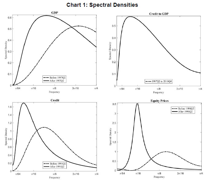  In case of credit-to-GDP ratio, the location of the peak is at 12.2 years. On the other hand, the periodogram of bank credit has seen a remarkable shift during the pre- and post-reform periods. The average length of main cycles in credit is measured at 15.1 years in post-1991 period as compared to much smaller cycles of about 5.4 years in the pre-1991 period. The amplitude and the spectral mass have also seen an increase for the range of 8 to 32 years. At peak, the amplitude is much higher for financial cycle than business cycle. The main cycle length of equity prices has also increased significantly from 3.4 years in pre-1991 period to 8.3 years in post-1991 period. In case of exchange rate, the main cycle length slightly increased from 3.1 years in pre-reform period to 3.6 years in the post-reform period. Further, the amplitude of equity price increased remarkably, while that of exchange rate remains more or less the same. Overall, the results from spectral analysis suggest that the average length of credit cycle is much longer than that of equity prices and exchange rate. Moreover, the length of cycle estimated from exchange rate is almost identical to the duration of business cycle. Credit-to-GDP ratio, house prices and equity prices experience cycles of much longer duration (particularly, in post-reform period) than business cycle but shorter relative to the credit cycle. As documented in the literature, we found the evidence suggesting business cycle to be shorter duration of 2 to 8 years as compared to credit cycle of 8 to 32 years. With the above observations from both turning point analysis and spectral density, we specify two ranges8 to extract short-term cycles (1 to 8 years range) and medium-term cycles (8 to 30 years range) using asymmetric band-pass filter as proposed by Christiano and Fitzgerald (2003). Essentially, the identification of short-term cycles in the data is motivated by the works of Comin and Gertler (2006) and Drehmann et al. (2012) in the context of business cycle and financial cycle, respectively. The idea behind extraction of both short- and medium-term cycles is to understand their relative importance in explaining the overall behavior of each variable. Therefore, we calculate volatility of the cycles using their standard deviations and compare the ratio of volatility of medium-term to that of the corresponding short-term cycles in each variables. We also provide a comparison between the relative volatilities in pre- and post-1991 period. To know how the volatility has evolved over time, the relative volatility of post-1991 over pre-1991 period is also calculated. Table 4 presents relative volatilities of individual variables. A ratio of greater than unity implies that medium-term cycles are more volatile (and have higher amplitudes) than the short-term cycles. A higher value of relative volatility indicates that a larger portion of variability of the series is explained by the medium-term cycles. The relative volatilities at 3.94 and 1.78 for credit and equity prices, respectively, are indicating the dominance of cycles at medium-term frequencies in explaining their overall variation. However, relative volatility has fallen significantly in the case of exchange rate suggesting a decline in importance of medium-term cycles in shaping exchange rate behaviour. A comparison between volatility of medium-term cycles for pre- and post-1991 period indicates that the amplitudes of medium-term cycles have risen in the post-reform period for all the variables (except exchange rate). In sum, the results suggest an increased dominance of medium-term cycles in explaining the overall behavior of financial variables in the post-reform period. | Table 4: Relative Volatility of Cycles | | Period | Credit | House Prices | Equity Prices | Exchange Rate | GDP | | Full Sample | 2.19 | 1.24 | 1.66 | 1.64 | 1.00 | | Pre-1991 | 1.40 | | 1.50 | 2.51 | 0.57 | | Post-1991 | 3.94 | 1.24 | 1.78 | 0.96 | 1.32 | | Post-1991 over Pre-1991* | 1.51 | | 1.35 | 0.42 | 1.32 | Relative volatility is calculated taking the ratio of standard deviations of medium-term to short-term cycles.
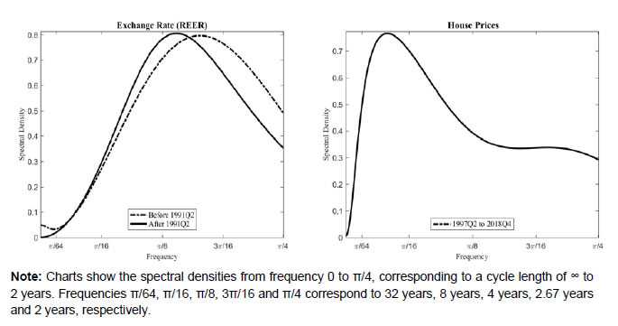
*: Ratio of standard deviations of medium-term cycles in pre- and post-1991 periods. | Measures of Financial Cycle With a view to construct an overall measure of financial cycle for India, medium to long term cycles of financial variables are extracted from individual series applying band-pass filter and specifying a band of 8 to 30 years. Chart 2 plots the extracted medium-term cycles for each variable. The medium-term cycle for credit witnessed an increase in both duration and amplitudes since mid-1990s as compared to earlier years. Medium-term equity price cycle has much higher amplitudes though the duration of the cycle has not changed over the years. On the other hand, medium-term cycles of exchange rate have weakened since mid-1990s. House price cycles, though have smaller amplitudes, last for several years. Taking the clue from these plots about the emergence of financial cycles in India since mid-1990s, we have combined the medium-term cycles of credit, equity prices and house prices using PCA to construct an aggregate measure of financial cycle. 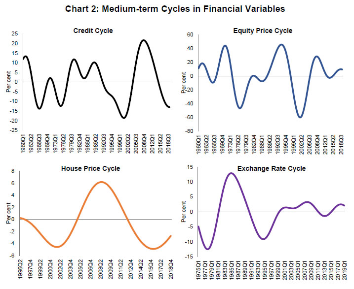 The medium-term cycles of the financial variables for common period, i.e., 1996Q2 through 2018Q4, are presented in Chart 3. Except for exchange rate, all other variables share common cyclical pattern and characteristics. The correlation coefficient between the cycles of credit and house prices is the highest at 0.86, followed by 0.66 between credit and equity price cycles and 0.63 between equity and house price cycles. This strong association is elucidated by the fact that the cycles share some common components. Such common feature, what financial cycle aims to capture, can be estimated by principal component analysis.  The above results provide the evidence of the existence of a financial cycle in India, particularly, in the post-1991 period. To obtain an aggregate/composite measure of financial cycle, the medium-term cycles of credit, house prices and equity prices are combined by using PCA.9 The factor loadings of the first principal component are used as weights to prepare the composite measure of financial cycle. The estimated first principal component explains about 58 per cent of combined variability in the financial data10. The normalised factor loadings from the PCA suggest strong weights for both credit and equity prices. Chart 4 presents an aggregate measure of financial cycle along with the contributions of individual components. While the overall financial cycle is mainly contributed by the credit and equity prices, house prices do not play a significant role. However, the role of house prices has increased since mid-2000s. The chart shows only one clear peak and one clear trough in aggregate financial cycle measure during 1996-2018. The application of turning point analysis on aggregate financial cycle reveals that there was only one peak at 2008:Q3 and two troughs in 2001:Q2 and 2017:Q1. It can also be inferred from the chart that the ongoing downturn in financial cycle seems to have reached its trough in 2018:Q4. 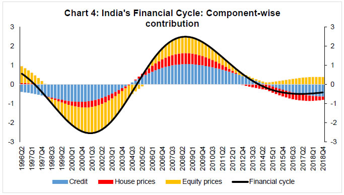 We construct another measure of financial cycle combining both credit and equity price cycles as long time-series data are available for these two variables. The alternative measure shows a strong co-movement with aggregate measure of financial cycle (Appendix III, Chart A1). The chart shows strong co-movement between these two measures of financial cycles. Employing turning point analysis on this alternative measure, we found that the average duration of contraction and expansion of financial cycle is about 24 quarters, each leading to the average length of financial cycles to about 12 years. The Chart A1 also shows that both amplitude and duration of financial cycles have increased with proliferation of financial liberalisation since the mid-1990s. Application of Financial Cycle The aggregate measure of financial cycle can be useful for several policy purposes, particularly as an early warning indicator for detecting exuberance or distress in the financial system. It is often found that business cycle recessions are much deeper when they coincide with the contraction phases of financial cycle (Claessens et al., 2012; Drehmann et al., 2012) and therefore, the peak of financial cycle may be seen as a warning sign for financial crisis or distress in the economy. On the other hand, GDP growth tends to be more stable in expansion phases of financial cycles with fading out of recession risks due to rise in asset prices and decline in leverage. In view of this, we examine the relationship between business and financial cycles. Further, the connection between financial cycle and non-performing assets is explored to gauge the predictable power of the latter in providing early warning signals about banking sector stress. Chart 5 plots both financial and business cycles11. The chart implies that the average duration of financial cycle is much longer than that of business cycle. The longer duration cycle being more persistent and having greater amplitudes could disrupt the structure of financial system immensely. In case it propagates to the business cycle frequency, it can increase the cost of output stabilisation. Additionally, the financial cycle seems to be more volatile (having greater amplitudes) than business cycle. On an average, the volatility of financial cycle is almost 1.5 times larger than that of the business cycle. The chart does not show a strong link between business cycle and financial cycle. Though the sharp downturn in business cycle in 2008 could have been driven by the global financial crisis, a part of this downturn and the weak economic activity in subsequent years could be seen as an evidence of early warning by the peak of the financial cycle in 2008:Q3. Also, there are periodic co-movement between business and financial cycles during 2002-2007 and 2011-2018. As long time series data are not available, it is difficult to find more such evidence in the short sample period of 22 years. However, as financial cycle is longer and its association with business cycle during downturn is severe, dampening of financial cycle through counter-cyclical policy measures is important to enhance macroeconomic and financial stability. 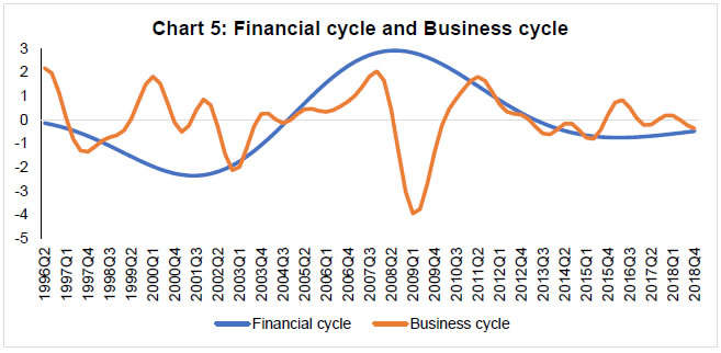 The relationship between financial cycle and business cycle is further examined by using Granger causality tests. The causality tests are conducted by taking the conventional business cycle (1 to 8 years duration) and the longer duration business cycle (8 to 30 years) with the aggregate measure of financial cycle. The results in Table 5 shows that there is no causal relationship between financial cycle and conventional business cycle. However, the evidence of bi-directional causality is found between financial cycle and longer duration business cycle. Moreover, the correlation between these two is 0.51, implying a strong association between the long-term cycles in economic and financial activities. | Table 5: Granger-Causality Test Results | | (Sample: 1996:Q2 to 2018:Q4) | Using Business Cycle of 1-8 years duration | Using Business Cycle of 8-30 years duration | | Null Hypothesis: | F-Statistic | P-value | F-Statistic | P-value | | Business Cycle does not Granger Cause Financial Cycle | 1.21 | 0.31 | 16465.30 | 0.00 | | Financial Cycle does not Granger Cause Business Cycle | 0.05 | 0.99 | 822.22 | 0.00 | | Note: Lag length of 4 is selected based on Schwarz Information Criteria. | According to Borio et al. (2018), “During expansions, the self-reinforcing interaction between financing constraints, asset prices and risk-taking can overstretch balance sheets, making them more fragile and sowing the seeds of the subsequent financial contraction. This, in turn, can drag down the economy and put further stress on the financial system”. Therefore, excess leverage ensues from the building up of debt stocks with lenders underestimating the potential risks of the borrowers and collaterals during the tranquil period. When asset prices fall, it reduces the value of collaterals and results in significant rise in leverages. Excess leverages finally burst and lead to financial distress. Financial cycle, which is an outcome of interactions between leverage and asset prices, is worth monitoring to understand the risks and also conduct suitable macro-prudential policies. Therefore, any sharp upturn of financial cycle needs to be monitored and contained. Similarly, buffers need to be maintained to manage the downturn phase. Chart 6 presents gross non-performing assets to total advances (GNPA) of the scheduled commercial banks along with the aggregate measure of financial cycle. It can be viewed from the chart that the upturn in financial cycle is accompanied by a reduction in stressed assets of banks during 2001-2008; and financial cycle reached its peak in 2008:Q3. The cycle entered into a contractionary phase thereafter. Though, it is difficult to draw precise inference from the limited number of turning points in financial cycle in India, it seems that lenders tend to have ignored the risks during the benign period i.e., the upturn phase of the financial cycle. This has resulted in high credit growth and subsequent rise in GNPA. A correct identification of turning points in financial cycle may, thus, provide a guidance for appropriate macro-prudential policies. VI. Conclusion The design and effectiveness of macro-prudential policies depend on how best we measure and understand the characteristics of financial cycle. In this study, we have attempted to determine the existence of financial cycle in India by examining the properties of financial cycle in different variables, viz. credit, credit-GDP ratio, equity prices, house prices and exchange rate. The empirical findings clearly indicate about the existence of financial cycle in India. We also find that the amplitudes of cycles in financial variables are much larger in expansion phase than in the contraction phase. The average duration of business cycle in India is about 5 years as compared to 15 years for credit cycle in the post-reform period. The length of cycles in exchange rate is nearly identical to the duration of business cycle whereas credit-to-GDP ratio and house prices experience cycles of much longer duration. On the other hand, equity prices have exhibited both short and medium-term cycles. We also find the rising dominance of medium-term cycles in explaining overall variation in credit and equity prices in the post-reform period. However, a weakening of the importance of medium-term cycles in shaping the exchange rate behaviour is observed since mid-1990s. Overall, the core empirical features of the cycles from individual variables suggest that there exists a financial cycle in India, which has gradually become more prominent with the proliferation of financial liberalisation since mid-1990s. The overall financial cycle of India can be best captured by the joint behaviour of credit, house prices and equity prices wherein credit and equity prices play the most significant role. Though house prices do not play a significant role, their importance in determining overall financial cycle has increased since mid-2000s. Overall, we find a longer duration financial cycle with the average length of about 12 years (6 years of expansion and 6 years of contraction) vis-à-vis a shorter duration business cycle with the overall average length of about 5 years. The analysis and the paper suggests that at the peak of the financial cycle provides some lead information about impending distress in the economy. Therefore, the policy should be designed to dampen financial cycle. A close monitoring of financial cycle on a regular interval is essential to enhance macroeconomic and financial stability.
References Aikman, D., Haldane, A. G., and Nelson, B. D. (2010). Curbing the Credit Cycle. Paper presented at the Columbia University Center on Capitalism and Society Annual Conference. New York. Aikman, D., Haldane, A. G., and Nelson, B. D. (2015). Curbing the Credit Cycle. Economic Journal, 125(585), 1072-1109. URL: https://EconPapers.repec.org/RePEc:wly:econjl:v:125:y:2015:i:585:p:1072-1109 Aizenman, J., Pinto, B., and Sushko, V. (2013). Financial Sector Ups and Downs and the Real Sector in the Open Economy: Up by the Stairs, Down by the Parachute. Emerging Markets Review, 16, 1-30. doi:https://doi.org/10.1016/j.ememar.2013.02.007 Alessi, L., and Detken, C. (2011). Quasi Real Time Early Warning Indicators for Costly Asset Price Boom/Bust Cycles: A Role for Global Liquidity. European Journal of Political Economy, 27(3), 520-533. doi:https://doi.org/10.1016/j.ejpoleco.2011.01.003 Anusha (2015). Credit and Growth Cycles in India and US: Investigation in the Frequency Domain. Paper presented at 11th ISI Annual Conference on Economic Growth and Development, URL: https://www.isid.ac.in/~epu/acegd2015/papers/Anusha.pdf. Banerjee, K. (2012). Credit and Growth Cycles in India: An Empirical Assessment of the Lead and Lag Behaviour. RBI Working Paper Series No. 22. Bhoi, B. K., and Behera, H. K. (2017). India’s Potential Output Revisited. Journal of Quantitative Economics, 15(1), 101-120. doi:10.1007/s40953-016-0040-9 Borio, C. (2012). The Financial Cycle and Macroeconomics: What Have We Learnt? BIS Working Papers(No. 395), Bank for International Settlements. URL: https://www.bis.org/publ/work395.htm Borio, C., Disyatat, P., and Juselius, M. (2016). Rethinking Potential Output: Embedding Information About the Financial Cycle. Oxford Economic Papers, 69(3), 655-677. doi:10.1093/oep/gpw063 Borio, C., and Drehmann, M. (2009). Assessing the Risk of Banking Crises - Revisited. BIS Quarterly Review, Bank for International Settlements, 29-46. URL: https://EconPapers.repec.org/RePEc:bis:bisqtr:0903e Borio, C., Drehmann, M., and Xia, D. (2018). The Financial Cycle and Recession Risk. BIS Quarterly Review, Bank for International Settlements. URL: https://EconPapers.repec.org/RePEc:bis:bisqtr:1812g Borio, C., Kennedy, N., and Prowse, S. D. (1994). Exploring Aggregate Asset Price Fluctuations across Countries: Measurement, Determinants and Monetary Policy Implications. BIS Economic Papers(No 40), Bank for International Settlements. URL: https://www.bis.org/publ/econ40.htm Borio, C., and Lowe, P. (2002). Assessing the Risk of Banking Crises. BIS Quarterly Review, Bank for International Settlements, 43-54. URL: https://EconPapers.repec.org/RePEc:bis:bisqtr:0212e Borio, C., and Lowe, P. (2004). Securing Sustainable Price Stability: Should Credit Come Back from the Wilderness? BIS Working Papers(No. 157), Bank for International Settlements. URL: https://EconPapers.repec.org/RePEc:bis:biswps:157 Burns, A. F., and Mitchell, W. C. (1946). Measuring Business Cycles: National Bureau of Economic Research, Inc. Christiano, L. J., and Fitzgerald, T. J. (2003). The Band Pass Filter*. International Economic Review, 44(2), 435-465. doi:10.1111/1468-2354.t01-1-00076 Claessens, S., Kose, M. A., and Terrones, M. E. (2011). Financial Cycles: What? How? When? NBER International Seminar on Macroeconomics, 7(1), 303-344. URL: https://EconPapers.repec.org/RePEc:ucp:intsma:doi:10.1086/658308 Claessens, S., Kose, M. A., and Terrones, M. E. (2012). How Do Business and Financial Cycles Interact? Journal of International Economics, 87(1), 178-190. doi:https://doi.org/10.1016/j.jinteco.2011.11.008 Comin, D., and Gertler, M. (2006). Medium-Term Business Cycles. American Economic Review, 96(3), 523-551. doi:10.1257/aer.96.3.523 de Winter, J., Koopman, S. J., Hindrayanto, I., and Chouhan, A. (2017). Modeling the Business and Financial Cycle in a Multivariate Structural Time Series Model. DNB Working Papers(No. 573), Netherlands Central Bank. URL: https://EconPapers.repec.org/RePEc:dnb:dnbwpp:573 Detken, C., and Smets, F. (2004). Asset Price Booms and Monetary Policy. ECB Working Papers(No 364), European Central Bank. URL: https://EconPapers.repec.org/RePEc:ecb:ecbwps:2004364 Drehmann, M., Borio, C., and Tsatsaronis, K. (2012). Characterising the Financial Cycle: Don't Lose Sight of the Medium Term! BIS Working Paper(No 380), Bank for International Settlements. URL: https://EconPapers.repec.org/RePEc:bis:biswps:380 Einarsson, B., Gunnlaugsson, K., Ólafsson, T., and Pétursson, T. (2016). The Long History of Financial Boom-Bust Cycles in Iceland - Part Ii: Financial Cycles. Central Bank of Iceland Working Papers(No. 72), Central bank of Iceland. URL: https://EconPapers.repec.org/RePEc:ice:wpaper:wp72 English, W., Tsatsaronis, K., and Zoli, E. (2005). Assessing the Predictive Power of Measures of Financial Conditions for Macroeconomic Variables. In Investigating the Relationship between the Financial and Real Economy (Vol. 22, pp. 228-252): Bank for International Settlements. Espinoza, R., Fornari, F., and Lombardi, M. J. (2012). The Role of Financial Variables in Predicting Economic Activity. Journal of Forecasting, 31(1), 15-46. doi:10.1002/for.1212 Galati, G., Hindrayanto, I., Koopman, S. J., and Vlekke, M. (2016). Measuring Financial Cycles in a Model-Based Analysis: Empirical Evidence for the United States and the Euro Area. Economics Letters, 145, 83-87. doi:https://doi.org/10.1016/j.econlet.2016.05.034 Goodhart, C., and Hofmann, B. (2008). House Prices, Money, Credit, and the Macroeconomy. Oxford Review of Economic Policy, 24(1), 180-205. URL: https://EconPapers.repec.org/RePEc:oup:oxford:v:24:y:2008:i:1:p:180-205 Harding, D., and Pagan, A. (2002). Dissecting the Cycle: A Methodological Investigation. Journal of Monetary Economics, 49(2), 365-381. doi:https://doi.org/10.1016/S0304-3932(01)00108-8 Hiebert, P., Klaus, B., Peltonen, T. A., Schüler, Y. S., and Welz, P. (2014). Capturing the Financial Cycle in Euro Area Countries. Financial Stability Review, 2, 109-117. URL: https://EconPapers.repec.org/RePEc:ecb:fsrart:2014:0002:2 Khundrakpam, J. K., Kavediya, R., and Anthony, J. M. (2017). Estimating Financial Conditions Index for India. Journal of Emerging Market Finance, 16(1), 61-89. doi:10.1177/0972652716686273 Menden, C., and Proaño, C. R. (2017). Dissecting the Financial Cycle with Dynamic Factor Models. Quantitative Finance, 17(12), 1965-1994. doi:10.1080/14697688.2017.1357971 Ng, T. (2011). The Predictive Content of Financial Cycle Measures for Output Fluctuations. BIS Quarterly Review, Bank for International Settlements, 53-65. URL: https://EconPapers.repec.org/RePEc:bis:bisqtr:1106g Pontines, V. (2017). The Financial Cycles in Four East Asian Economies. Economic Modelling, 65, 51-66. doi:https://doi.org/10.1016/j.econmod.2017.05.005 Schularick, M., and Taylor, A. M. (2012). Credit Booms Gone Bust: Monetary Policy, Leverage Cycles, and Financial Crises, 1870-2008. American Economic Review, 102(2), 1029-1061. doi:10.1257/aer.102.2.1029 Schüler, Y., Hiebert, P. H., & Peltonen, T. (2017). Coherent Financial Cycles for G-7 Countries: Why Extending Credit can be an Asset. Working Paper No. 43. European Systemic Risk Board. Schüler, Y., Hiebert, P. P., and Peltonen, T. (2015). Characterising the Financial Cycle: A Multivariate and Time-Varying Approach. ECB Working Papers(No 1846), European Central Bank. URL: https://EconPapers.repec.org/RePEc:zbw:vfsc15:112985 Stremmel, H. (2015). Capturing the Financial Cycle in Europe. ECB Working Paper(No. 1811), European Central Bank. URL: https://www.ecb.europa.eu//pub/pdf/scpwps/ecbwp1811.en.pdf Strohsal, T., Proaño, C., and Wolters, J. (2017). Characterizing the Financial Cycle: Evidence from a Frequency Domain Analysis. IMK Working Paper(No. 189), Macroeconomic Policy Institute. URL: https://EconPapers.repec.org/RePEc:imk:wpaper:189-2017
Appendix I: Chronology of Cycles in India | Table A1: Dates of Turning Points in Financial Variables and GDP | | Variables | Credit | House Prices | Equity Prices | Exchange Rate | GDP Growth | | Peaks | Troughs | Peaks | Troughs | Peaks | Troughs | Peaks | Troughs | Peaks | Troughs | | | 1964Q1 | 1964Q4 | 2001Q1 | 2001Q2 | 1962Q1 | 1968Q1 | 1977Q1 | 1976Q1 | 1982Q1 | 1982Q3 | | | 1967Q1 | 1967Q3 | 2003Q1 | 2003Q3 | 1969Q2 | 1970Q1 | 1981Q2 | 1979Q1 | 1983Q4 | 1985Q1 | | | 1973Q4 | 1974Q4 | 2008Q3 | 2009Q1 | 1970Q3 | 1971Q4 | 1983Q4 | 1982Q2 | 1985Q4 | 1986Q2 | | | 1991Q2 | 1992Q1 | 2014Q3 | 2016Q1 | 1972Q2 | 1973Q2 | 1985Q2 | 1984Q4 | 1987Q1 | 1988Q1 | | | 1993Q2 | 1994Q2 | | | 1973Q4 | 1975Q2 | 1988Q1 | 1987Q3 | 1988Q4 | 1989Q2 | | | 1998Q2 | 1998Q4 | | | 1976Q4 | 1977Q4 | 1990Q2 | 1989Q2 | 1990Q1 | 1991Q2 | | | 2008Q4 | 2009Q4 | | | 1979Q1 | 1980Q2 | 1994Q2 | 1992Q2 | 1992Q2 | 1993Q1 | | | | | | | 1981Q4 | 1984Q2 | 1997Q3 | 1996Q1 | 1994Q1 | 1995Q3 | | | | | | | 1986Q1 | 1988Q1 | 2001Q2 | 1998Q4 | 1996Q2 | 1997Q2 | | | | | | | 1990Q3 | 1991Q1 | 2003Q3 | 2003Q1 | 2000Q1 | 2001Q1 | | | | | | | 1992Q2 | 1993Q2 | 2005Q3 | 2004Q3 | 2002Q1 | 2002Q4 | | | | | | | 1994Q3 | 1996Q4 | 2007Q3 | 2006Q3 | 2003Q4 | 2004Q4 | | | | | | | 1997Q3 | 1998Q4 | 2011Q3 | 2008Q4 | 2007Q2 | 2009Q1 | | | | | | | 2000Q1 | 2001Q4 | 2013Q1 | 2012Q2 | 2010Q1 | 2013Q1 | | | | | | | 2002Q2 | 2003Q1 | 2017Q4 | 2013Q3 | 2016Q1 | 2017Q2 | | | | | | | 2007Q4 | 2008Q4 | | | 2018Q1 | | | | | | | | 2010Q4 | 2012Q2 | | | | | | | | | | | 2013Q1 | 2013Q3 | | | | | | | | | | | 2015Q1 | 2016Q1 | | | | | | | | | | | 2018Q3 | | | | | | | Duration | | | | | | | | | | | | Expansion | 26.83 | | 16.33 | | 5.84 | | 6.13 | | 5.07 | | | Contraction | 3.14 | | 2.75 | | 6.05 | | 5.36 | | 4.53 | | | | | | | | | | | | | | | Amplitudes | | | | | | | | | | | | Expansion | 75.79 | | 34.78 | | 43.72 | | 7.91 | | 6.20 | | | Contraction | -4.67 | | -6.59 | | -36.42 | | -11.00 | | -6.35 | |
Appendix II: Spectral Decomposition Spectral or frequency-domain analysis is a statistical technique of converting a stationary time-series into a combination of sinusoids. This is closely related to the Fourier analysis, in which (deterministic) functions are decomposed into combination of sinusoids. In this paper, we adopted the approach of indirect estimation of spectral densities, as delineated by the Strohsal et al. (2015). The first part of this approach is to specify the data generating process of the underlying time series as an ARMA model. ARMA representation can be interpreted as a filter of infinite length which depends only on finite number of parameters. In this way ARMA model act as a tractable filter which captures the whole dynamics of the observed series. The (ARMA) model specification procedure follows the principle of parsimony. As reported in Tables A2, all parameters in the final specifications are statistically significant at standard confidence levels and the estimated residuals are free from autocorrelation according to the Lagrange multiplier (LM) test. The second part of this approach is to obtain spectral densities from the estimated ARMA. It is known that any covariance-stationary process has a time domain and a frequency domain representation which are fully equivalent. Given this, the frequency domain representation is more suited to the analysis of cyclical features, as the importance of certain cycles for the total variation of the process can be easily derived from the spectrum12. In order to provide an example, consider the estimated ARMA model of Indian credit growth during the pre-1991 period, These estimates are used to calculate the spectrum f(λ) of the ARMA process, which is given by the following relation: 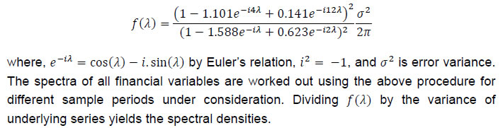 | Table A2: ARMA Specifications | | Parameters | GDP | Credit | Equity Price | REER | House Price | Credit/GDP | | Pre-reform Period | | constant | 5.160
(23.9) | 9.912
(16.4) | | | | | | AR(1) | 0.513
(3.7) | 1.589
(21.6) | 0.953
(34.5) | 1.490
(12.3) | | | | AR(2) | | -0.629
(-8.49) | | -0.466
(-3.65) | | | | MA(4) | -0.903
(-36.4) | -1.101
(-15.4) | -1.085
(-48.5) | -1.680
(-24.0) | | | | MA(8) | | | | 0.723
(12.1) | | | | MA(12) | | 0.141
(2.03) | 0.480
(26.4) | | | | | diagnostics | | | | | | | | LM(4) | 0.49 | 0.81 | 0.74 | 0.15 | | | | LM(8) | 0.51 | 0.98 | 0.48 | 0.43 | | | | LM(12) | 0.12 | 0.99 | 0.76 | 0.50 | | | | Post-reform Period | | constant | 7.182
(54.9) | 10.840
(6.47) | 438.334
(104.32) | 0.792
(7.28) | | | | AR(1) | 0.885
(21.2) | 1.193
(33.09) | 1.467
(15.64) | 0.831
(14.03) | 0.671
(6.34) | 0.284
(2.90) | | AR(2) | | | -0.404
(-3.47) | | 0.267
(2.46) | 0.434
(3.86) | | AR(4) | | -0.212
(-5.87) | | -0.109
(-2.54) | | 0.213
(1.82) | | AR(5) | | | -0.118
(-3.78) | | | | | MA(4) | -0.980
(-41.5) | -0.943
(-38.2) | -0.931
(-45.0) | -0.974
(-72.3) | -0.849
(-10.7) | -0.602
(-4.96) | | MA(8) | | | | | | -0.351
(-3.01) | | MA(12) | | | | | -0.133
(-1.72) | | | diagnostics | | | | | | | | LM(4) | 0.63 | 0.14 | 0.61 | 0.15 | 0.22 | 0.71 | | LM(8) | 0.88 | 0.10 | 0.50 | 0.22 | 0.55 | 0.89 | | LM(12) | 0.67 | 0.32 | 0.79 | 0.49 | 0.59 | 0.62 | | Note: Figures in parentheses under the parameter estimates are t-statistics. LM: Lagrange Multiplier Q- statistics. | The estimated spectral densities as shown in Chart 1 are in the range [0, π/4], i.e. for period of ∞ to 2 years. The conventional business cycle range of 2 to 8 years corresponds to the frequency interval [π/16, π/4] and financial cycle range of 8 to 32 years corresponds to [π/64, π/16], and the classification of the frequency ranges are based on Strohsal et al. (2015). ------------------------------------------
Appendix III |