“… the primary objective of the monetary policy is to maintain price stability while keeping in mind the objective of growth.” [Excerpted from Preamble to the Reserve Bank of India (RBI) Act, 1934
(amended by the Finance Act, 2016)] 1. Introduction II.1 Under FIT in India, monetary policy has to accord primacy to the goal of price stability, with due consideration to the objective of growth. The country experience yields several examples of inflation targeting frameworks with dual mandates. This performance record is replete with testing challenges and conflicting pulls inherent in the trade-offs between these objectives. There are also some central tendencies. Growth as an objective of monetary policy is found to have never been quantified, unlike the inflation target. It has also never been set as the primary goal in the mandate of monetary policy. Inflation targets and tolerance bands around them are, on the other hand, clearly defined in quantitative terms. The country experience also reveals another tendency that has evolved over time – targets/bands have mostly declined/narrowed over time1, incentivised by the success achieved in stabilising headline inflation and inflation expectations, and the drive to catch up with the best in class. II.2 In India, CPI-C inflation averaged 3.9 per cent during the period of FIT (October 2016 – March 2020)2. Over this period, GDP growth underwent a sustained deceleration from 8.3 per cent in 2016- 17 to 4.0 per cent in 2019-20, including a 44-quarter low of 3.1 per cent during January-March 2020. In the context of these outcomes, attention has been drawn to the ‘sacrifice ratio’, i.e., the sacrifice of output necessary for disinflating from some higher reaches of an inflation experience towards the numerical target that defines price stability. In India, the RBI has been criticised for unusually high real interest rates during the FIT period (Government of India, 2018; Bhalla, 2017); FIT being inimical to growth (Bhattacharya et al., 2020); mindless monetary dogmatism, which could have been avoided if an explicit growth target was also mandated along with the inflation target (Jagannathan, 2019); and, imposing a potential constraint to achieving the medium-term goal of a US$ 5 trillion economy (Agarwala, 2020). Even around the time when an explicit inflation target was adopted, concerns were expressed about its relevance for a country with young population (Singh, 2014); that microeconomic foundations of CPI based inflation targeting were not empirically tested robustly before its adoption (Srinivasan, 2014); and that the target needed to be higher, particularly the lower band, given the structural nature of inflation in India (Panagariya, 2015). The actual experience with FIT in India has swung the pendulum more recently. It has been highlighted that neither did the RBI neglect changes in the output gap nor did monetary policy become hawkish after the adoption of FIT (Eichengreen et al., 2020). II.3 The next review of the inflation target, which is a core element of FIT, is due before March 31, 2021. Reassessing the inflation target and the tolerance band, is the most important motivation of this chapter. Under the Agreement on the Monetary Policy Framework signed by the RBI and the Government of India (GOI) on February 20, 2015, it was specified that: (a) the Reserve Bank will aim to bring inflation below 6 per cent by January 2016; and (b) that the inflation target for India for 2016-17 and all subsequent years shall be 4 per cent with a band of (+/-) 2 per cent. In the subsequent amendment of the RBI Act, this institutional framework was endorsed. Section 45ZA of the Act clearly specified that “The Central Government shall, in consultation with the Bank, determine the inflation target in terms of the Consumer Price Index, once in every five years. The Central Government shall, upon such determination, notify the inflation target in the Official Gazette.” The provisions of the amended RBI Act were brought into force through a notification in the Gazette of India on June 27, 2016. The inflation target of 4 per cent and the lower and upper tolerance bands were set at 2 per cent and 6 per cent, respectively, in a Gazette notification on August 5, 2016 valid for the period beginning from the date of publication of the notification and ending on March 31, 2021. A review of the inflation target is, thus, embedded in this Gazette notification. II.4 It is important to recognize that while setting a single target/tolerance band for the next five years, structural changes that may materialise or the type of shocks that may hit the economy are difficult to anticipate fully. Hence, flexibility must be built into the framework, without undermining the discipline of the inflation target, which has to be forward-looking to ensure that inflation expectations are firmly anchored over the medium term to facilitate decisions on investment, savings and consumption. It is important to revisit the target periodically, even when a review is not required by statute, because changing underlying structural characteristics of the economy and inflation dynamics can render the target sub-optimal. II.5 Another motivation of this chapter stems from the deceleration of growth during FIT, which poses several intriguing empirical questions. In our view, clarity on them is essential if the suitability of the framework for the future has to be justified: (a) did FIT contribute to the slowdown in growth? (b) would a higher inflation target ab initio have been more appropriate for India’s growth dynamics? and (c) is the current inflation target consistent with the goal of achieving a US$ 5 trillion economy? II.6 This chapter is, accordingly, organised into seven sections. Section 2 reviews the experiences of IT countries and their strategies to keep monetary policy relevant in swiftly changing macro-financial conditions. Section 3 focuses on the determination of appropriate inflation target using the concept of trend inflation. Section 4 evaluates the tolerance band on the basis of three conditioning aspects: (a) food and fuel shocks to the inflation path; (b) structural and statistical analysis of the inflation process; and (c) projection errors over different time horizons. Section 5 dwells on other features of the inflation process – persistence and expectations. The consistency of the inflation target with the growth objective is examined in Section 6. The concluding section sets out policy perspectives and recommends the inflation target, and the tolerance band for the next five years. 2. Country Experience 2.1 Inflation Target II.7 IT in practice has undergone several transformations over the past three decades, often driven by periodic reviews, but more by ‘learning by doing’. These changes have been reflected in amendments of the inflation targets and operating frameworks covering the range of policy instruments, their deployment under specific macro-financial conditions, and the decision-making process. II.8 Country-specific inflation targets have evolved over time in response to the exigencies of localised circumstances and conditioned by the interaction with global macroeconomic developments. While AEs have generally established inflation targets in the range of 1-3 per cent, EMEs adopted higher targets, typically against the backdrop of higher inflation histories. EMEs too have gradually reduced their inflation targets over time, drawing upon the success achieved in stabilising headline inflation and expectations. Many EMEs have successfully married inflation targeting frameworks with foreign exchange interventions, thereby innovating within the IT tradition to seek out intermediate solutions to the impossible trinity. II.9 Broadly, countries have adopted three kinds of targets, viz., point targets; point targets with tolerance bands; and range targets (Chart II.1). Several central banks have also changed the type of target in response to changing inflation dynamics, and particularly so in response to the nature and size of shocks to the inflation trajectory. The majority of IT-practicing EMEs have adopted point targets with tolerance bands, as opposed to most AEs that have preferred inflation targets of 2 per cent with narrow/no tolerance band. II.10 As stated earlier, EMEs have gradually reduced their inflation targets to a range of 2-4 per cent in South America and South-East Asia (Chart II.2a and b). Only in Brazil, the inflation target was raised in 2003 in response to domestic unrest and the 9/11 shock to mitigate sharp exchange rate depreciation. This increase in target was short-lived and it was reduced again after 2004. II.11 Eastern European countries have also progressively reduced their targets to converge to a range of 2.5-4.0 per cent (Chart II.2c). While inflation targets in AEs have remained relatively stable over the last two decades (Chart II.2d), Norway deliberately set its target above that of other major European economies in 2001, when it faced a period during which substantial oil revenues were to be phased into the economy. Norway reduced its inflation target in 2018 to 2.0 per cent from 2.5 per cent earlier, as the country’s liberal spending from oil revenues was contained, dampening pressure on prices. 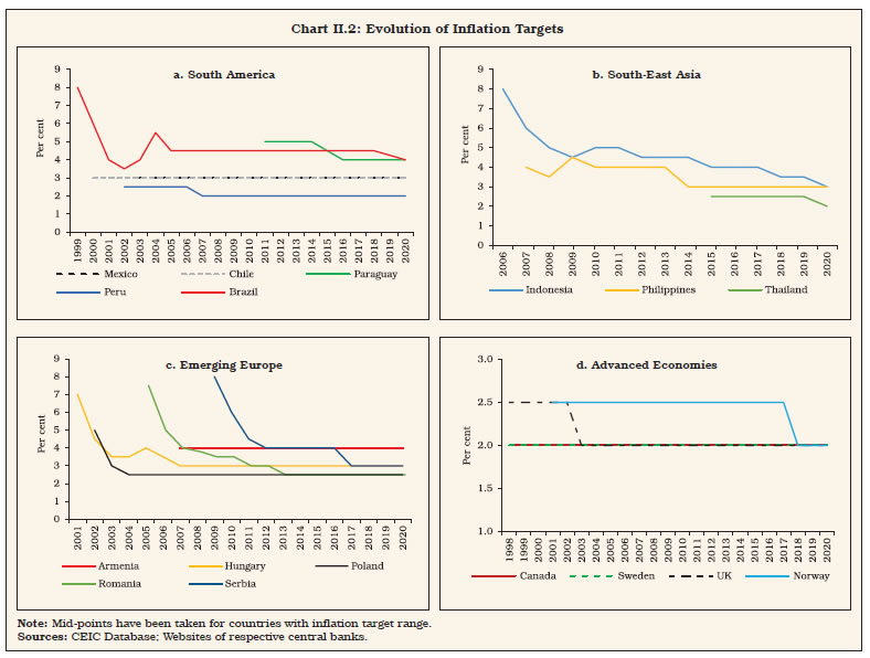 II.12 Several countries have quite regularly reviewed and changed both levels of the target and the width of their tolerance bands. Illustratively, South Korea, which adopted IT in 1998, shifted from a point target with a tolerance band to a narrower range target in 2004 (Chart II.3a). In 2007, the Bank of Korea (BoK) moved away from targeting core inflation to headline inflation, and also adopted a point target with a fluctuation band (3.0 +/-0.5 percentage points). The tolerance band was widened to +/- 1 percentage point amidst high inflation volatility, while maintaining the 3.0 per cent target for the period 2010-12. Subsequently, it shifted back to a narrow target band and in 2016, it lowered the inflation target to 2.0 per cent without any tolerance band (Ciżkowicz-Pękała et al., 2019). II.13 Among South-East Asian countries, a broader target band aimed to provide flexibility in steering inflation. The Bangko Sentral ng Pilipinas (BSP) shifted from a range target to a point target with a tolerance interval of ±1 percentage point starting 2008 (Chart II.3b), which effectively widened the target band (BSP, 2019). II.14 Thailand adopted IT in the year 2000 with core inflation as the target. Thailand narrowed the target range for core inflation in 2009 from 0-3.5 per cent to 0.5-3.0 per cent (Chart II.3c). The lower bound of the target range was adjusted upwards by 0.5 percentage points to reduce the likelihood of deflation. In 2015, the target was shifted from core to headline inflation of 2.5 per cent with a tolerance band of ± 1.5 per cent, which was subsequently changed to a range of 1.0-3.0 per cent for 2020, prompted by long periods of divergence of core inflation from headline inflation. The choice of the latter was also conditioned by the fact that it reflected changes in the cost of living better and was used as a reference for consumption and saving decisions by households, and for investment and price setting decisions by businesses. The switch from a range to a point target was intended to give a clearer signal to the public regarding the commitment of monetary policy towards maintaining price stability, which should help strengthen its effectiveness in anchoring the public’s long-term inflation expectations. Re-adoption of range target in 2020 intended to provide more monetary policy flexibility amidst volatile and uncertain global economic conditions. The Czech Republic shifted from a range target to a point target, and also gradually reduced its target (Chart II.3d). 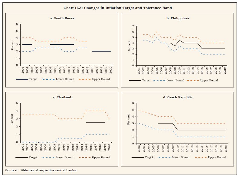 2.2 Tolerance Band II.15 Most EMEs have a tolerance band around their mandated inflation targets, the motivation being to formally incorporate flexibility into their policy frameworks (Table II.1). Overwhelmingly, the preference is for symmetrical tolerance bands – deviations in both direction from the target are treated in the same way. On the width of the band, +/- 1 per cent dominates, although some countries also have wider bands. There are outliers too – while Georgia and Russia have point targets without any tolerance band, Jamaica, South Africa, Thailand and Uruguay have the band as the target. II.16 In many EMEs, food constitutes a sizeable component of CPI – around 32 per cent on average – as compared with the AE average of around 19 per cent (Table II.1). This renders the former prone to supply shocks. Their experience also suggests that a higher food share in the CPI is associated with relatively higher inflation targets and wider tolerance bands. It is not very common for countries to change or revise their tolerance band, unlike in the case of the inflation target (Chart II.4). | Table II.1: Inflation Target and Tolerance Band for EMEs | | EMEs with Higher Share of Food in CPI | EMEs with Lower Share of Food in CPI | | Sr. No | EME | Share of Food in CPI (per cent) | Inflation Target (per cent) | Tolerance Band (per cent) | Sr. No | EME | Share of Food in CPI (per cent) | Inflation Target (per cent) | Tolerance Band (per cent) | | 1 | India | 45.9 | 4.0 | +/-2.0 | 13 | Uganda | 28.5 | 5.0 | +/-2.0 | | 2 | Ukraine | 45.0 | 5.0 | +/- 1.0 | 14 | Paraguay | 26.9 | 4.0 | +/-2.0 | | 3 | Ghana | 43.9 | 8.0 | +/-2.0 | 15 | Uruguay | 26.0 | 3.0 - 7.0 | | | 4 | Philippines | 38.3 | 3.0 | +/- 1.0 | 16 | Mexico | 25.8 | 3.0 | +/- 1.0 | | 5 | Jamaica | 37.5 | 4.0-6.0 | | 17 | Poland | 25.2 | 2.5 | +/- 1.0 | | 6 | Albania | 37.3 | 3.0 | +/- 1.0 | 18 | Peru | 25.1 | 2.0 | +/- 1.0 | | 7 | Thailand | 36.1 | 1.0 - 3.0 | | 19 | Indonesia | 25.0 | 3.0 | +/-1.0 | | 8 | Egypt | 32.7 | 7.0 | +/- 2.0 | 20 | Dominican Republic | 23.8 | 4.0 | +/- 1.0 | | 9 | Serbia | 31.2 | 3.0 | +/- 1.5 | 21 | Turkey | 22.8 | 5.0 | +/-2.0 | | 10 | Georgia | 31.0 | 3.0 | | 22 | Hungary | 21.5 | 3.0 | +/- 1.0 | | 11 | Russia | 31.0 | 4.0 | | 23 | Chile | 19.3 | 3.0 | +/- 1.0 | | 12 | Brazil | 31.0 | 3.75 | +/- 1.5 | 24 | South Africa | 17.2 | 3.0 - 6.0 | | | | | | | | 25 | Colombia | 15.1 | 3.0 | +/- 1.0 | | Sources: www.centralbanknews.info and IMF. |
 II.17 Currently, only two countries have escape clauses incorporated into their inflation targeting frameworks, viz., Czech Republic and Romania, in addition to a tolerance band. Incidentally, both countries have escape clauses included in their Fiscal Responsibility and Budget Management (FRBM) frameworks as well. 3. The Inflation Target II.18 Trend inflation is the permanent or the underlying component of inflation to which actual inflation converges after a shock. Alternatively referred to as steady state inflation (Ascari and Sbordone, 2014), it is consistent with the potential level of output, the natural rate of unemployment and the natural rate of interest. Consequently, it provides a valuable guide for monetary policy authorities in assessing the appropriate level of the inflation target. A target fixed much below the trend could produce a deflationary bias in the economy while a target set above the trend level renders monetary policy too expansionary and prone to inflationary shocks (Behera and Patra, 2020). In fact, there is an influential view that setting the target above the trend could increase inflation and its volatility, undermining the confidence of firms and households to undertake and execute long-term plans, squandering the credibility of the central bank, destabilising inflation expectations and raising risk premiums in asset markets (Bernanke, 2010). As a result, the effects of shocks on macroeconomic variables could become more persistent (Ascari and Sbordone, 2014). The optimal approach is to set the inflation target in close alignment with the trend inflation (Tulasi et al., 2021). II.19 Trend inflation, however, is unobservable and hence an empirical issue, warranting careful choice of methodology and sample period for estimation in order to secure precision if it has to serve as the metric for setting the inflation target, especially to avoid costly policy errors. These choices have to be sensitive to the regime changes and structural shifts that underlie the inflation process. First, the relationship between inflation and economic growth is non-linear (Phillips, 1958; Okun, 1962); hence, the use of any linear approach to measure trend inflation could produce imprecise estimates. Second, the incidence of sporadic supply shocks further complicates the measurement of trend inflation by producing noise. Estimating trend inflation involves filtering out the noise in inflation data, but there are multiple sources of noise and the nature of the noise can change over time. Thus, it embodies a signal extraction problem (Stock and Watson, 2016). Third, the time varying nature of the trend makes estimation even more challenging as it is difficult to distinguish sources of inflation that are persistent from those that are transitory3. II.20 The most popular method of estimation of trend inflation is the unobserved components stochastic volatility (UCSV) model (Stock and Watson, 2007)4. Using different variants of unobserved components models on monthly data on headline CPI (y-o-y)5, trend inflation estimates are obtained in the range of 3.8 – 4.3 per cent for the FIT period (Chart II.5 and Table II.2). II.21 Trend inflation can also be estimated through multivariate approaches that combine cross sectional and time series properties of different inflation measures such as headline CPI inflation, WPI inflation and the GDP deflator in the Indian case but preserve the unique properties of the UCSV model. The underlying assumption is that inflation measured by different indicators converges to the same trend. The questions that multivariate approaches seek to address are: Will there be improvements by using different inflation measures? Do the implied weights evolve over time, or are they stable? Do these trend inflation measures improve on the UCSV estimates? The multivariate unobserved components model estimated here allows for common persistent and transitory factors and time-varying factor loadings in the common and index specific components. The time-varying factor loadings allow for changes in the co-movements across measures, such as the reduction in energy price pass-through into other prices. A strength of the method is that the resulting estimates adjust for changes in persistence of the component series (Stock and Watson, 2016). The estimated average trend inflation obtained from this multivariate approach using data for the period 1981:Q2 through 2020:Q2 works out to 3.9 per cent during FIT period (Chart II.5). | Table II.2: Trend Inflation Estimates of India | | Models | Estimates for 2020:Q1 | | UCSV | 4.2 | | UCSV-MA (Stochastic Volatility in Inflation) | 4.1 | | UCSV-MA (Stochastic Volatility in Inflation and Trend) | 4.3 | | Multivariate unobserved components model | 3.8 | | Regime switching (with only inflation) | 4.2 | | Regime switching (with NKPC) | 4.1 – 4.3 | | Source: RBI staff estimates. |
II.22 The multivariate model improves upon the UCSV model by bringing information from various inflation measures. As noted in the literature, however, improvements in accuracy of estimation, especially in forecasting are small relative to the computation burden. II.23 The Bai-Perron structural break test6 identifies four structural breaks7 in India’s inflation series, with the last structural break point in 2014:Q3 coinciding with the de facto adoption of FIT in India (Chart II.6). II.24 A recent strand in the empirical literature has sought to estimate trend inflation by modelling it as influenced by extrinsic macroeconomic conditions embodied in the Phillips curve. Rather than a purely forward-looking NKPC advocated in the theoretical literature, a hybrid Phillips curve is preferred. In a recent effort, regime shifts in monetary policy are introduced into the Phillips curve through a Markov Chain Monte Carlo (MCMC) process (Behera and Patra, 2020). Estimates from this model yield trend inflation in India at 4.1-4.3 per cent (Box II.1). II.25 Based on these alternative estimates, the observed decline in trend inflation since 2014 and a decline in inflation persistence as shown in Section 5 indicate that households and businesses in India are becoming more forward-looking than before as credibility associated with monetary policy is increasing – it is appropriate to maintain the inflation target at 4 per cent into the medium-term. Box II.1
Trend Inflation in India Trend inflation is regarded as a key building block of the New Keynesian model that is at the core of the monetary policy frameworks of modern central banks across the world. Measuring trend inflation is essentially an empirical issue, with attention being increasingly given to precision in modelling the time-varying dynamics of trend inflation including structural shifts therein. In the theoretical literature, the standard approach has been to assume zero trend inflation in the steady state. In the empirical literature, however, a non-zero trend inflation is preferred and a wide variety of models for estimating trend inflation from the data is available. Survey-based data on inflation expectations have been used but estimates of trend inflation therefrom suffer from various biases in the survey responses. Survey-based approaches also lack several positive features of a model such as ascertaining the determinants of trend inflation and obtaining a forecast when needed. Trend inflation has also been measured by the last period’s inflation rate; as a random walk; a random walk subject to bounds; and as an exponentially smoothed trend. The workhorse model for estimating trend inflation, and arguably the most popular, has been the unobserved components with stochastic volatility (UCSV) model. The trend is defined as a random walk8 process, while the inflation gap is governed by a separate process of stochastic volatility, i.e., it has no persistence. Extension of the UCSV model has involved a so-called ‘multivariate’ approach designated as the multivariate stochastic volatility model, which has been estimated for India in the foregoing. For the purpose of measuring trend inflation in India in the presence of shifts in inflation dynamics, a hybrid New Keynesian Phillips curve (NKPC) is estimated on quarterly data for the period 1981:Q2 through 2020:Q1 in which current inflation depends on lagged inflation to capture the historical intrinsic behaviour of the inflation process, trend inflation to reflect persistence in inflation expectations and the contemporaneous output gap to represent the extrinsic macroeconomic conditions relevant for the setting of monetary policy. The hybrid NKPC is specified as follows: 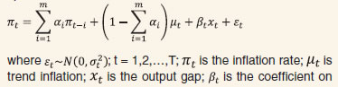 
 Before estimating the NKPC model with pre-specification of regimes, a Markov switching regression with unknown regimes is estimated to understand the current regime of inflation. The results indicate two regimes in India’s recent inflation history – a high inflation regime of 9.4 per cent during 2007-2014 and a low inflation regime of 4.0 per cent since 2015 (Chart 1). The probability weighted estimate of trend inflation in the current regime is 4.2 per cent. The real time estimate of trend inflation is 4.1 per cent in Q1 of 2020. Smoothed probability weighted estimates of trend inflation eased steadily from 2009 to reach 4.3 per cent in Q1 of 2020 (Chart 2). Hence, the estimate of trend inflation for India is 4.1-4.3 per cent. The decline in trend inflation since 2014 is coincident with a flattening of the Phillips curve. Underlying this is (a) a decline in the inflation persistence, indicating that households and businesses in India are becoming more forward-looking than before as credibility associated with monetary policy increases; and (b) an increase in the sacrifice ratio – further disinflations will become costlier in terms of the output foregone. At the same time, the credibility bonus accruing to monetary policy warrants smaller policy actions to achieve the target. This points to maintaining the inflation target at 4 per cent into the medium-term. Reference: Behera, H.K. and Patra, M.D. (2020), “Measuring Trend Inflation in India”, RBI Working Paper Series, No. 15, December. | 4. The Tolerance Band II.26 Having identified the appropriate level of the target for inflation, we now turn to the tolerance bands around the target within which actual inflation outcomes will be allowed to deviate from the target while minimising the losses of output. The need for defining a tolerance band is primarily based on three considerations. First, the band allows flexibility to the central bank to look through temporary fluctuations caused by supply shocks. Second, the band should accommodate the actual inflation within it for most of the time without undermining credibility of the central bank. Third, inflation forecasts act as the intermediate target in a FIT regime (Svensson, 1997). Consequently, the deviation of forecasts from realised inflation – forecast errors – is not just a factor in assessing the performance of inflation targeting but also informs the framework itself by affecting the tolerance band. The tolerance band can hence be considered as a “confidence interval”9. As a result, the width of the band should reflect a conscious and judicious balance between flexibility and credibility. 4.1 The Upper Tolerance Level II.27 The relationship between inflation and economic growth is non-linear – up to some low level of inflation, it is positive, i.e., some benign rate of price increase is beneficial for growth by greasing the wheels of production with reasonable returns. Per contra, at some higher rate of inflation, growth decelerates and can even turn negative if inflation rises further – large changes in prices create uncertainty that impedes consumption and investment decisions. Hence, even after setting the target in alignment with the steady state inflation, it is important to fix the upper bound up to which rising inflation is associated with smaller increases in growth till it reaches its maximum, beyond which inflation becomes growth retarding. This growth-inflation trade-off provides the motivation for locating the threshold, i.e., the kink beyond which inflation is unambiguously inimical to growth. Precision in estimating the threshold is critical in order to numerically set the upper bound for deviations from the inflation target. II.28 Empirical estimates of threshold inflation for India that are available in the literature range between 4 and 7 per cent across different time periods (Annex II.1). Updated estimates of threshold inflation using alternative methodologies (Box II.2 and Annex II.2) found it to lie in the range of 4 – 5 per cent for the sample period 2002:Q2 to 2020:Q1, and 5 – 6 per cent for a longer sample period 1997:Q2 to 2020:Q1. As the concept of threshold inflation applies to the long run and growth is unambiguously impaired when inflation crosses 6 per cent, it is recommended that 6 per cent be maintained as the appropriate upper tolerance limit for India’s inflation target to remain credible (Table II.3). Box II.2
Estimates of Threshold Inflation for India Drawing on the literature (Rangarajan, 1998; 2020), a number of approaches are used to work out threshold inflation for India. They also serve to provide robustness checks. (a) Splining Among the methodologies employed to estimate threshold regression, splining involves a series of regression equations to identify the threshold value of inflation based on maximum R-squared or minimum Root Mean Square Error (RMSE) (Sarel, 1996). Following Khan and Senhadji (2001), the following equation is estimated: where year-on-year growth in GDP (GDPgt) is regressed on its lag, change in lagged credit to GDP ratio (∆cred_gdpt) to explain the impact of financial development on growth, lagged inflation level (πt) and a dummy variable interacting with deviation of inflation from a pre-specified threshold level (π*) as part of the search process. The dummy variable takes a value of 1 if the realised inflation is above the threshold level and 0 otherwise. The threshold value is pre-specified in the range of 3 – 8 per cent levels and the maximum adjusted R-squared for any threshold value is considered as the optimum. The results, based on data for the sample period Q2:2002 to Q1:2020 indicate a point of inflection at 5 per cent (Chart 1 and Table 1). 
| Table 1: Parameter Estimates | | Threshold Levels | 3.0 | 3.5 | 4.0 | 4.5 | 5.0 | 5.5 | 6.0 | 6.5 | 7.0 | 7.5 | 8.0 | | Constant | -0.18 | 0.28 | -0.17 | 0.3 | 0.85 | 1.32 | 1.64* | 1.96* | 2.18** | 2.37** | 2.58** | | GDPgt-1 | 0.53*** | 0.52*** | 0.52*** | 0.53*** | 0.53*** | 0.53*** | 0.53*** | 0.53*** | 0.53*** | 0.53*** | 0.54*** | | ∆cred_gdpt-1 | 0.14 | 0.14 | 0.13 | 0.14 | 0.15 | 0.15 | 0.15 | 0.15 | 0.15 | 0.16 | 0.16 | | CPI_INF(-1) | 1.20 | 0.93 | 0.99 | 0.80** | 0.62** | 0.48** | 0.39* | 0.31* | 0.25 | 0.19 | 0.14 | | Threshold | -1.21 | -0.96 | -1.07* | -0.92** | -0.77** | -0.67** | -0.62* | -0.56* | -0.53* | -0.49 | -0.43 | | D2002Q3 | -3.32*** | -3.38*** | -3.53*** | -3.66*** | -3.79*** | -3.89*** | -3.74*** | -3.61*** | -3.51*** | -3.41*** | -3.33*** | | D2003Q3 | 3.19*** | 3.13*** | 2.97*** | 2.83*** | 2.70*** | 2.71*** | 2.85*** | 2.96*** | 3.03*** | 3.08*** | 3.13*** | | D2009Q1 | -3.97*** | -3.94*** | -3.84*** | -3.74*** | -3.67*** | -3.63*** | -3.60*** | -3.59*** | -3.56*** | -3.54*** | -3.57*** | | D2010Q1 | 5.70*** | 5.76*** | 5.89*** | 6.00*** | 6.07*** | 6.12*** | 6.18*** | 6.19*** | 6.21*** | 6.20*** | 6.14*** | | Adj. R2 | 0.511 | 0.516 | 0.530 | 0.536 | 0.537 | 0.535 | 0.533 | 0.529 | 0.527 | 0.523 | 0.518 | ***, **, *: Significant at 1 per cent, 5 per cent and 10 per cent levels, respectively.
Different dummy variables are also used to incorporate outlier effects.
Source: RBI staff estimates. | (b) Logistic Smooth Transition Regression (LSTR) The Logistic Smooth Transition Regression (LSTR) model (Teräsvirta, 1994; Eitrheim and Teräsvirta, 1996) estimates the threshold level of inflation and also the speed of transition from one regime (low effect of inflation on growth) to another (high effect of inflation on growth). The basic difference from the spline model is that instead of using a dummy variable to differentiate the regimes, weights are assigned on the basis of a logistic function that allows the parameter to differ across regimes, enabling identification of the threshold. The functional form of the model can be specified as: 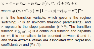 The results imply that there exists a nonlinear relationship between inflation and growth as the null hypothesis of linearity is rejected at 5 per cent significance level (Table 2). The nonlinearity in the growth-inflation relationship is also confirmed by the statistical significance of the slope parameter. The estimated threshold value of inflation from this regression works out to 5.0 per cent. | Table 2: Estimated Parameters in LSTR Model | | | Coefficient | t-statistic | | Threshold: π* | 4.97*** | 2.75 | | Slope: γ | 0.37* | 1.80 | | Variable | | | | Inflation (πt-1) (< threshold) | 1.62** | 2.63 | | Inflation (πt-1) (> threshold) | -1.19** | -2.05 | | GDP growth (yt-1) | 0.25* | 1.68 | | GDP growth (yt-1) | 0.55*** | 2.79 | | OECD GDP growth | -1.15*** | -3.05 | | Dstructural | 4.97*** | 2.75 | | R2 | 0.54 | | | DW | 1.77 | | | LM(4) P-val | 0.30 | | | ARCH(4) P-val | 0.25 | | | Test of Linearity and Non-linearity | | | Test of Linearity
(p-value) | Test of remaining Nonlinearity
(p-value) | | Terasvirta Sequential Tests | 0.02 | 0.42 | | Escribano-Jorda Tests | 0.05 | 0.13 | H0: β2 = 0 or γ = 0
Source: RBI staff estimates. | (c) Threshold VAR (TVAR) In multivariate frameworks like threshold VAR (TVAR), threshold inflation is computed from the estimated nonlinear impulse responses which are derived as conditional forecasts at each period. Hence, it is possible to study time variance in responses to shocks not only across regimes, but also within regimes. Moreover, it is possible to test whether nonlinearities are statistically significant. Another advantage of the TVAR methodology is that the variable by which different regimes are defined can itself be an endogenous variable included in the VAR. Therefore, regime switches may occur after the shock to each variable. The TVAR can be specified as: Using Bayesian methods and treating inflation as the threshold variable, the estimated threshold level works out to 4.5 per cent (Chart 2). An exogenous shock to inflation causes GDP growth to fall under the high inflation regime (i.e. when inflation is above 4.5 per cent). On the contrary, the growth impact is positive when inflation is below 4.5 per cent. The cumulative impact (over 12 quarters) of one percentage point rise in inflation on GDP growth is: (+)37 bps under the low inflation regime and (-)46 bps under the high inflation regime. While the positive impact is statistically insignificant, the negative effects are significant for most lags. (d) Panel Threshold Regression Considerable heterogeneity in the inflation and growth experiences of Indian states has encouraged estimation of the threshold inflation at the sub-national level (Mohaddes and Raissi, 2014). In a panel framework, using data on GSDP growth and CPI inflation across major Indian states for the period 2011-12 to 2018-19, the following equation is estimated:
Table 3: Panel Regression Estimates
(Dependent Variable: GDP growth) | | | (π*=3) | (π*=3.5) | (π*=4) | (π*=4.5) | (π*=5) | (π*=6) | | π | 2.295 | 1.876* | 1.428* | 1.069* | 0.676 | 0.277 | | | (1.655) | (1.036) | (0.754) | (0.639) | (0.557) | (0.484) | | D×(π- π*) | -2.628 | -2.240** | -1.818** | -1.475* | -1.103 | -0.753 | | | (1.688) | (1.085) | (0.831) | (0.758) | (0.723) | (0.771) | | Constant | -0.593 | -0.331 | 0.452 | 1.262 | 2.812 | 4.660 | | | (5.950) | (4.455) | (3.699) | (3.383) | (3.136) | (2.974) | | R2 (Overall) | 0.3009 | 0.3086 | 0.3115 | 0.3111 | 0.3036 | 0.2951 | | N | 154 | 154 | 154 | 154 | 154 | 154 | Standard errors in parentheses; * p < 0.10, ** p < 0.05, *** p < 0.01;
Sample: 2011-12 to 2018-19 for 22 states.
Source: RBI staff estimates. | References Eitrheim, Ø., and Teräsvirta, T. (1996), “Testing the Adequacy of Smooth Transition Autoregressive Models”, Journal of Econometrics, Vol. 74(1), 59-75. Khan, M. S., and Senhadji, A. S. (2001), “Threshold Effects in the Relationship Between Inflation and Growth”, IMF Staff Papers, Vol. 48(1), 1-21. Mohaddes, M. K., and Raissi, M. M. (2014), “Does Inflation Slow Long-Run Growth in India? (No. 14-222)”, International Monetary Fund. Rangarajan, C. (1998), “Development, Inflation and Monetary Policy”, in I. Ahluwalia, and I. Little, India’s Economic Reforms and Development: Essays for Manmohan Singh, New Delhi: OUP. Rangarajan, C. (2020), “The New Monetary Policy Framework-What it Means”. Journal of Quantitative Economics, Vol. 18, No.2, May 2020, pp. 457-470. Sarel, M. (1996), “Nonlinear effects of inflation on economic growth”. IMF Staff Papers, Vol. 43(1), 199-215. Teräsvirta, T. (1994), “Specification, Estimation, and Evaluation of Smooth Transition Autoregressive Models”, Journal of the American Statistical association, Vol. 89(425), 208-218. | II.29 For India, model-based estimates of the upper tolerance level for inflation need to be conditioned by the vulnerability of the economy to recurring supply shocks such as weather adversities and/or volatility in international commodity prices. The agricultural sector is still heavily dependent on rainfall as merely 49 per cent of the gross cropped area is irrigated. Inefficiencies in the food supply chain – high and volatile retail mark ups on wholesale/farm gate prices and limited level of development of the food processing industry – also impact food inflation (Bhoi et al., 2019; Dhanya et al., 2020). With the highest share of food in the consumption basket in the world (45.9 per cent) and high volatility in food inflation – 3.2 as against 1.4 for headline inflation during the FIT period (Chart II.7) – there is a strong case for a wider tolerance band for India relative to the country experience. | Table II.3: Threshold Inflation Estimates of India | | Method | Expert Committee Report | Current Estimates using CPI Inflation | | WPI Inflation | CPI Inflation | Recent Period
(2002:Q2 to 2020:Q1) | Full Sample
(1997:Q2 to 2020:Q1) | | LSTR | 5.8 | 6.7 | 5.0 | 5.6 | | Threshold VAR | 4.6 | 6.2 | 4.5 | 5.5 | | Spline Regression | | | 5.0 | 6.0 | | Panel Threshold Model | | | 4.0 | 5.0 | | Source: RBI staff estimates and Expert Committee report. |
II.30 Food inflation remained within the tolerance band only about 43 per cent of the time in the FIT period – inflation in respect of pulses, vegetables and sugar remained within the tolerance band less than 20 per cent of the time. In fact, for vegetables and pulses price volatility has increased in the FIT period, mainly on account of an increase in extreme weather events (Table II.4 and Chart II.8). | Table II.4: Performance of Different Food Sub-Groups during Pre and Post - FIT | | Item | Weight | Inflation above 6 per cent
(in per cent of months) | Inflation below 2 per cent
(in per cent of months) | Inflation within 2 to 6 per cent
(in per cent of months) | | Pre -FIT | Post-FIT | Pre -FIT | Post-FIT | Pre -FIT | Post-FIT | | CPI All Groups | 100 | 57.9 | 7.1 | 0.0 | 4.8 | 42.1 | 88.1 | | Food and Beverages | 45.86 | 71.9 | 14.3 | 1.8 | 42.9 | 26.3 | 42.9 | | Cereals and products | 9.67 | 45.6 | 0.0 | 10.5 | 26.2 | 43.9 | 73.8 | | Meat and fish | 3.61 | 78.9 | 33.3 | 0.0 | 4.8 | 21.1 | 61.9 | | Egg | 0.43 | 57.9 | 38.1 | 19.3 | 40.5 | 22.8 | 21.4 | | Milk and products | 6.61 | 75.4 | 4.8 | 0.0 | 28.6 | 24.6 | 66.7 | | Oils and fats | 3.56 | 33.3 | 7.1 | 19.3 | 50.0 | 47.4 | 42.9 | | Fruits | 2.89 | 63.2 | 21.4 | 15.8 | 35.7 | 21.1 | 42.9 | | Vegetables | 6.04 | 61.4 | 40.5 | 22.8 | 45.2 | 15.8 | 14.3 | | Pulses and products | 2.38 | 71.9 | 21.4 | 7.0 | 71.4 | 21.1 | 7.1 | | Sugar and confectionery | 1.36 | 31.6 | 35.7 | 56.1 | 50.0 | 12.3 | 14.3 | | Spices | 2.50 | 73.7 | 14.3 | 15.8 | 47.6 | 10.5 | 38.1 | | Non-alcoholic beverages | 1.26 | 47.4 | 0.0 | 0.0 | 26.2 | 52.6 | 73.8 | | Prepared meals, snacks, sweets etc. | 5.55 | 89.5 | 2.4 | 0.0 | 2.4 | 10.5 | 95.2 | Note: Pre-FIT period covers January 2012 - September 2016.
Sources: NSO; RBI staff estimates. |
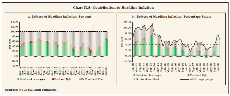 II.31 The contribution of food, and particularly, vegetables, to volatility10 in headline inflation11 is significantly higher than non-food items, reflecting the perishable nature of the crop, short crop cycles, lack of adequate storage and poor pre-and post-harvest practices (Chart II.9). Even non-perishables such as pulses and cereals have exhibited considerable volatility. II.32 Apart from food, another major source of supply shock to inflation in India is fuel prices, with more than 80 per cent of domestic oil consumption met through imports. Fluctuations in petroleum product prices in India reflect not only movements in global crude prices, but also changes in excise duties and value added tax (VAT) as well as the exchange rate of the rupee. The fuel and light group has a weight of around 7 per cent in the CPI basket, which mainly comprises electricity, firewood and chips, LPG and kerosene (Chart II.10). It is the transport and communication subgroup in the CPI that is directly impacted by changes in the prices of petroleum products as it contains petrol and diesel. 4.2 The Lower Tolerance Level II.33 For the determination of the lower tolerance bound, it is necessary to investigate the statistical properties of the inflation process under the deflationary impact of structural shocks. II.34 Adapting from the tradition of the seminal work on shocks and frictions in business cycles within the framework of a structural dynamic stochastic general equilibrium model (Smets and Wouters, 2007), the lower tolerance level for inflation in India can be estimated by assessing the impact of supply shocks on production costs and pricing. There appears to be a minimum level of inflation below which producers are unable to pass on changes in production costs to selling prices. Estimates for India for the period 1996:Q2 to 2019:Q2 indicate that the magnitude12 of supply shocks varies from (+) 1.56 to (-) 1.56 per cent, where the former denotes the upper bound and the latter denotes the lower bound. The impulse response results imply that the impact of supply shocks on inflation mainly persists for four quarters, with a band of (+/-) 2.18 per cent around the target accommodating supply shocks 90 per cent of the time (Chart II.11). This is the level of inflation on account of supply-side factors (such as unexpected changes in oil prices, raw materials, imported intermediates and the like) which cannot be influenced by monetary policy. Any attempt to bring down inflation below this level using contractionary monetary policy would dis-incentivise production activity as firms would not be able to pass on increased costs to final consumers. A lower bound of above 2 per cent will lead to actual inflation frequently dipping below the tolerance band (as explained in the next section), while a lower bound below 2 per cent will hamper output/growth13. In the history of the CPI (base 2012=100), inflation has not fallen below 2 per cent in any quarter14.  II.35 These estimates can be counterfactually corroborated by evaluating the symmetry or otherwise of the tolerance band. Drawing on monthly data through the history of the CPI series, it is observed that the distribution of the transitory component of inflation – estimated by taking the deviation of actual year-on-year inflation from its trend15 – is found to be centred around zero with a probability value of 0.8 for inflation observations lying between -2 and +2 per cent (Chart II.12). The skewness and kurtosis tests for normality confirm that the distribution of cyclical components of inflation is symmetric around zero and normally distributed. This supports a symmetric tolerance band set at +/- 2 percentage points around the inflation target so that actual inflation will remain above the lower bound and below the upper bound 80 per cent of the time. These results also suggest that, given the estimate of trend inflation at 4 per cent, the model derived estimate of the upper tolerance level has a downside bias and needs to be revisited by juxtaposing it with actual outcomes. 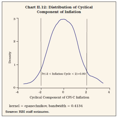 II.36 Finally, the assessment of forecasting performance carried out in Chapter III can inform the choice of the width of the tolerance band, which is a function of forecast errors. The observed incidence of these errors leave little space for narrowing of the existing +/- 2 per cent tolerance band. The empirical assessment of accuracy and efficiency of inflation forecasts conducted during FIT shows that forecast errors up to 1.88 per cent are inherent in the projection processes, validating the adoption of +/- 2 per cent tolerance band (Table II.5). 5. Other Features of India’s Inflation Process II.37 The estimates of trend inflation and upper and lower thresholds help to define the primary mandate for FIT in India and to assess the success or otherwise in achieving it. In this regard, two other aspects of the inflation process merit consideration; first, the time taken for deviations of inflation from the target to correct or inflation persistence, and second, what beliefs/expectations do people hold about inflation and the ability of the central bank/ government in keeping it low and stable. 5.1 Inflation Persistence II.38 Inflation persistence is determined by intrinsic factors (i.e., past inflation behaviour) as well as extrinsic factors (the credibility of monetary policy in achieving the inflation target). In advanced economies, inflation persistence was reduced/ eliminated after the adoption of inflation targeting (Bratsiotis et al., 2002). In emerging economies in the Asia pacific region, inflation targeting countries witnessed significant decline in inflation persistence, unlike countries that did not adopt inflation targeting (Gerlach and Tillmann, 2011). Understanding the nature of inflation persistence, therefore, is important to evaluate the role of FIT in India. II.39 In technical terms, inflation persistence emanates from four sources. First, there is backward-lookingness in wage and price setting – wage negotiations typically take into account inflation of the recent past; firms revise their prices infrequently in response to recent sizeable changes in prices. This is termed as “intrinsic” persistence. Second, extrinsic inflation persistence relates to the mark-up over costs. Third, “expectations-based” persistence is due to private agents in the economy perceiving inflation to be different from the central bank’s target. Fourth, persistence can arise due to supply shocks (Angeloni et al., 2006). Another dimension of persistence may arise from monetary policy itself through interest rate smoothing or small and gradual interest rate changes in one direction to reinforce the intent of monetary policy (Patra et al., 2014)16. II.40 Empirical results suggest that in India17, intrinsic persistence declined when the FIT period is added to the pre-FIT sample period, whereas the role of expectations has risen18 (Table II.6). The lower value of the interest rate smoothing parameter appears to have contributed to the observed stabilisation of inflation expectations and thereby to the credibility of the FIT regime. II.41 In view of the short period covered under FIT restricting degrees of freedom, estimates of trend inflation within the UCSV tradition can be generated from an augmented Phillips curve in a time-varying parameter regression framework with stochastic volatility (TVP-SV)19 (Stock and Watson, 2007; Cogley, Primiceri and Sargent, 2010). Estimates show that the intrinsic persistence has declined contributing to the moderation in trend inflation (Chart II.13a). II.42 The decline in extrinsic persistence points to a softening of nominal rigidities in price setting (Chart II.13b). Stochastic volatility in inflation had started to decline much before FIT (Chart II.13c) because of fewer instances of unfavourable supply shocks in the recent past. 5.2 Inflation Expectations II.43 Households, firms and financial market players incorporate their inflation expectations into their decisions to consume, invest and change financial market positions. FIT focuses on anchoring inflation expectations of the public through a credible commitment to a publicly announced inflation target. This increases the probability of maintaining price stability on a durable basis. Several benefits can accrue: wage-price spirals can be averted; idiosyncratic supply shocks can be accommodated, and as a result the risk of growth sacrifices for achieving price stability can be minimised; and stability of financial markets can be engendered, facilitating efficient allocation of resources in the economy (Miyajima and Yetman, 2018). Cross-country Experience II.44 Both advanced and emerging economies show somewhat similar performance in anchoring of inflation expectations, before and after the adoption of an inflation targeting framework. Expectations of professional forecasters generally stabilise around the inflation target relatively quickly while expectations of households generally exceed the inflation target/ upper tolerance band, often taking several years to moderate after formal adoption of inflation targeting (Charts II.14 and II.15). Among AEs, it is only in New Zealand that households’ inflation expectations have eased to levels within the target band in recent years. A similar pattern is observed in South Africa while in Russia, households’ expectations continue to hover above the inflation target. In some countries, inflation expectations have most often tended to stay higher than both actual inflation and the inflation target. 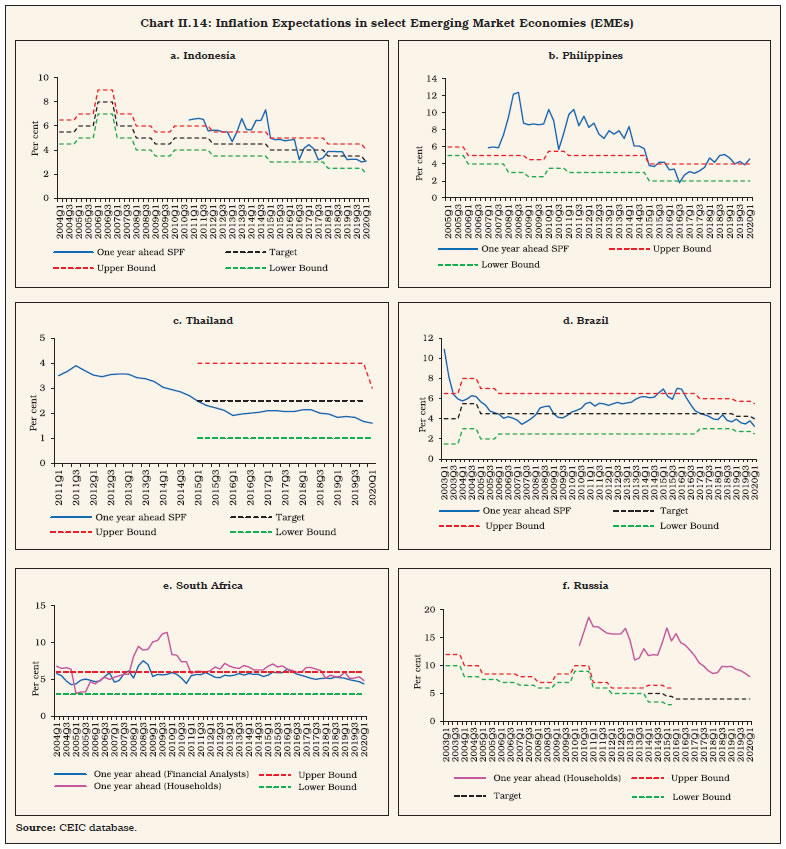
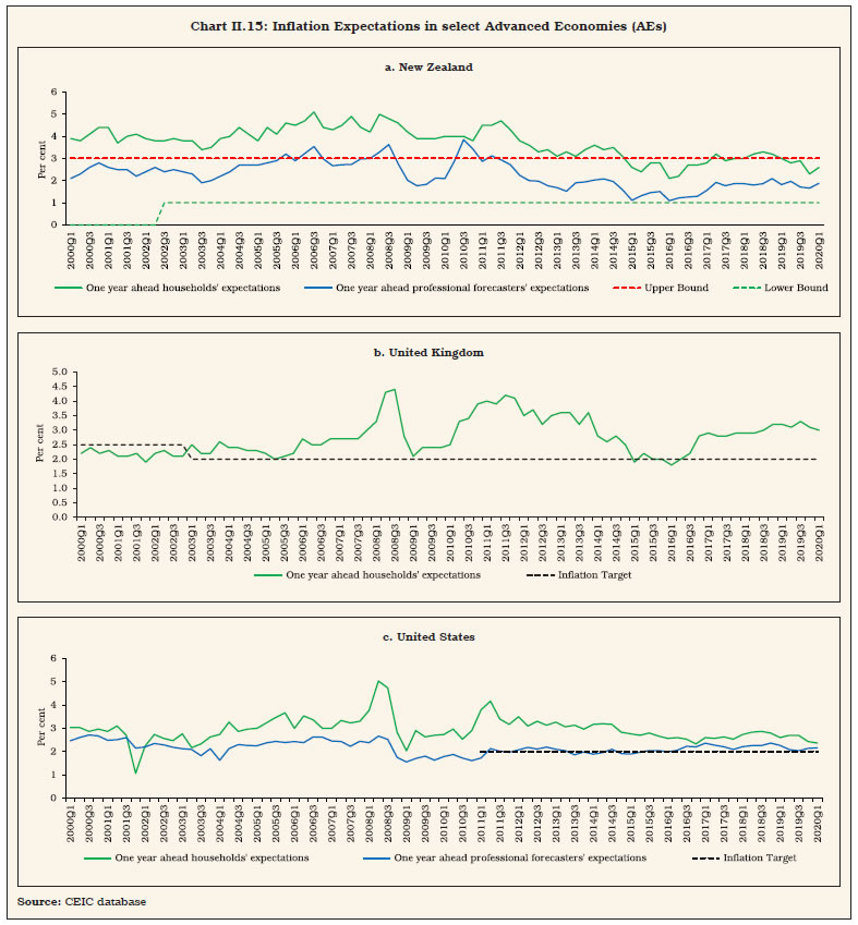 II.45 Overall, it is observed that across AEs and EMEs, households have a higher bias and lower degree of anchoring relative to professional forecasters and financial analysts. Inflation Expectations in India during FIT II.46 The Reserve Bank conducts bi-monthly surveys to collect information on inflation expectations of households (IESH) and professional forecasters (SPF)20. During the FIT period, current inflation perception of households has persistently remained above all official measures of inflation, imparting an upside to inflation expectations (i.e., inflation expectations for three months ahead and one year ahead are formed on the basis of current perceptions rather than actual inflation experienced as per official inflation data) (Chart II.16). On the other hand, expectations of professional forecasters have hovered around the actual inflation trajectory (Chart II.17). Households’ and professional forecasters’ sentiments on one year ahead inflation are strongly related, with a high and significant correlation of 0.79. 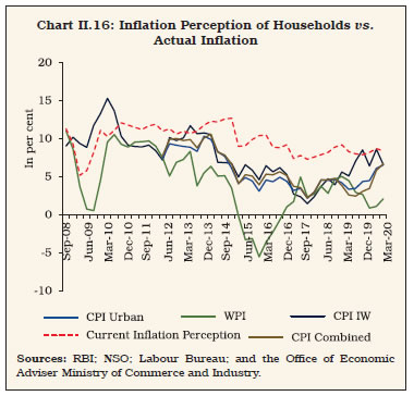 II.47 Since 2014, a decline in inflation expectations has trailed the fall in headline inflation (Chart II.18 and Table II.7). Statistically, inflation perception and inflation expectations exhibit a high degree of correlation with CPI-C headline inflation (Table II.7).
| Table II.7: Correlation between Inflation Expectations (IE) and Actual Inflation | | Correlation | CPI-C Headline | CPI-C Food | CPI-C Fuel | CPI-C Core | CPI- IW | WPI | | IESH Current Perception | 0.83 | 0.77 | 0.47 | 0.68 | 0.44 | 0.47 | | IESH one quarter ahead IE | 0.87 | 0.78 | 0.53 | 0.75 | 0.45 | 0.50 | | IESH one year ahead IE | 0.90 | 0.83 | 0.57 | 0.75 | 0.43 | 0.51 | | SPF one quarter ahead IE | 0.78 | 0.59 | 0.27 | * | * | 0.91 | | SPF one year ahead IE | 0.26 | 0.29 | 0.01 | * | * | 0.42 | * In SPF, forecast of CPI-IW was included till December 2013. Subsequently, in place of CPI-IW, forecast of CPI-C headline and CPI-C core were requested for.
Sources: RBI; NSO; Labour Bureau and the Office of Economic Adviser in the Ministry of Commerce and Industry. | II.48 The anchoring of one year ahead inflation expectations across professional forecasters and households during the FIT period has enhanced the efficacy of monetary policy (Box II.3). Box II.3
Stabilisation of Inflation Expectations during FIT in India To assess whether FIT has helped in stabilising inflation expectations, the following regression specification is used: 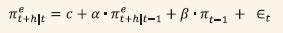 Considering that regime changes are often gradual, the above equation is estimated allowing for model parameters to vary over time. The model is estimated for both one quarter ahead and one year ahead inflation expectations of households and professional forecasters. The time-varying parameter estimates show that the beta (β) parameter – signifying the influence of actual inflation on inflation expectations (IE) – has dropped significantly from peak levels of 2010-2014, for one year ahead inflation expectations of both households and professional forecasters (Chart 1c and d). From mid-2014, the beta (β) parameter has gradually declined and remained statistically significant up to mid- 2017. Hence, the adoption of FIT has led to an enhancement in monetary policy transparency which is associated with an improved degree of anchoring of inflation expectations in India (Samanta and Kumari, 2021). In order to explore the level of inflation expectations around which one year ahead expectations have stabilized post- FIT, the following model is used: where αt depicts the time-varying trend level of expectations. This slow-moving trend indicates the long-term level around which expectations have been stabilized. The resulting time-varying estimates for alpha (α) parameter confirms stabilisation of IE around the range of 9-10 per cent for households and 4-5 per cent for professional forecasters (Chart 2). Lastly, anchored inflation expectations can be both ‘shock anchored’ and ‘level anchored’ (Ball and Mazumder, 2011; Chen, 2019). Testing this hypothesis, the inflation outlook of professional forecasters is found to be both shock and level anchored, while households’ expectations were susceptible to fuel price shocks, based on recent experiences (Table 1a and b). 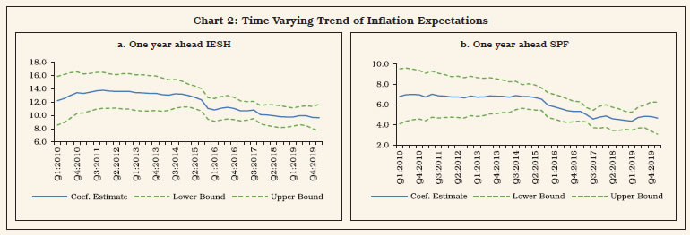
| Table 1a: Test for ‘Shock Anchored’ Inflation Expectations of Households | | IE1YH = c + β1CPIIWEX + β2CPIIWF + β3CPIIWT + εt | | Period | c | CPIIWEX | CPIIWF | CPIIWT | Adj. R2 | | Q2:2009-10 to Q2:2016-17 | 10.357 [0.000] | -0.179 [0.377] | 0.123 [0.147] | 0.363 [0.003] | 0.417 | | Q3:2016-17 to Q4:2019-20 | 7.601 [0.000] | -0.055 [0.536] | 0.192 [0.092] | 0.224 [0.044] | 0.213 | IE1YH : One year ahead mean inflation expectations of households
CPIIWEX : Four quarter lagged CPI-IW inflation-excluding ‘food’, ‘fuel and light’ and ‘transport and communication’
CPIIWF : CPI-IW inflation of subgroup ‘food’ for the previous month
CPIIWT : CPI-IW inflation of subgroup ‘transport and communication’ for the previous month | Figures in brackets are p-values.
Source: RBI staff estimates. |
| Table 1b: Test for ‘Shock Anchored’ Inflation Expectations of Professional Forecasters | | IE1YS = c + β1CPIIWEX + β2CPIIWF + β3CPIIWT + β4CPIIWFl + εt | | Period | c | CPIIWEX | CPIIWF | CPIIWT | CPIIWFl | Adj. R2 | | Q2:2009-10 to Q2:2016-17 | 3.471 [0.000] | -0.059 [0.295] | 0.223 [0.000] | -0.000 [0.993] | 0.233 [0.000] | 0.810 | | Q3:2016-17 to Q4:2019-20 | 5.000 [0.000] | -0.125 [0.001] | 0.101 [0.083] | 0.023 [0.696] | -0.043 [0.316] | 0.693 | IE1YS : One year ahead mean inflation expectations of professional forecasters
IE1YS : Two quarter lagged value of CPI-IW inflation of subgroup ‘food’
CPIIWT : Two quarter lagged value of CPI-IW inflation of subgroup ‘transport and communication’
CPIIWFl : Two quarter lagged value of CPI-IW inflation of subgroup ‘fuel and light’ | Figures in brackets are p-values.
Source: RBI staff estimates. | References: Ball, L. and Mazumder, S. (2011), “Inflation Dynamics and the Great Recession”, Brookings Papers on Economic Activity 42 (Spring), 337–405. Chen, Y.G. (2019), “Inflation, Inflation Expectations and the Phillips Curve”, Congress Budget Office, Washington, D.C., Working Paper Series 2019-07. Samanta, G. P., and Kumari, S., (2021), “Monetary Policy Transparency and Anchoring of Inflation Expectations in India”, Reserve Bank of India Working Papers No 03/2021. | 6. The Objective of Growth II.49 Given the dual mandate of FIT, there has been considerable debate as to whether primacy assigned to price stability contributed to the growth slowdown. The absence of a quantitative target for growth, unlike for inflation, impedes an objective assessment of the debate. Hence, this section turns to a review of the experiences of inflation targeting countries to explore the possibility of drawing lessons therefrom in order to evaluate the central issue of the debate referred to above. 6.1 Country Experience II.50 In several inflation targeting countries, growth is not explicitly stated as an objective of monetary policy. In some others, their objectives include growth explicitly (Annex II.4). Whether stated explicitly or implicitly, however, it has never been quantified or set as a numerical target, unlike the inflation target. Furthermore, growth is never reported as the primary objective of monetary policy. In policy communication, most central banks are emphatic that by keeping inflation low, stable and predictable, monetary policy can create an appropriate environment to stimulate investment and achieve long-term sustainable economic growth. II.51 In Australia, the objective of monetary policy is to set interest rate in a way that best contributes to the stability of the currency (price stability), full employment, and the economic prosperity and welfare of the people of Australia. In New Zealand, besides price stability, monetary policy is mandated to support maximum sustainable employment. Under operational objectives, it explicitly requires the MPC to consider a broad range of labour market indicators with the realisation that the maximum sustainable employment is not directly measurable. The explicit goals of monetary policy of the US Federal Reserve are to promote maximum employment, stable prices and moderate long-term interest rates. In the UK, the main aim of monetary policy is to maintain low and stable inflation to support the government’s main objective to achieve strong, sustainable and balanced growth. In the post- GFC low inflation environment, policy attention has turned increasingly to growth in advanced and emerging economies alike, justifying the use of ultra-accommodative monetary policy. Even so, neither has growth been set as the primary objective of monetary policy nor has the growth objective been quantified. II.52 There is an overwhelming consensus that monetary policy cannot raise long-term (or potential) growth (Papademos, 2003). It can only reduce the variability of output around the potential (Meyer, 2001). The best contribution of monetary policy to growth is through low and stable inflation (Lacker, 2014). There is also an alternative view that a temporary shortfall in demand, unless stabilised in a timely manner, can lead to a permanent loss of output through hysteresis effects21 (Garga and Singh, 2021). Monetary policy shocks can trigger long-run effects on total factor productivity, capital accumulation and overall productive capacity of an economy (Jorda et al., 2020). Monetary policy under FIT tends to be asymmetric – too tight during recessions and not so loose during expansions – generating a downward impulse to aggregate demand and the resultant negative real effects on output growth (Libanio, 2010). II.53 In India, sustained deceleration in GDP growth during the FIT period requires empirical examination of the role of monetary policy. A specific indicator that could help in this assessment is the level of the real policy interest rate during and before FIT. 6.2 Real Policy Interest Rate II.54 The real policy rate remained persistently positive during the FIT period (excluding last two quarters), whereas in the pre-FIT period, the real policy rate was negative for a long period (Chart II.19)22. Is lower investment and GDP growth during FIT attributable to the positive real policy rate? 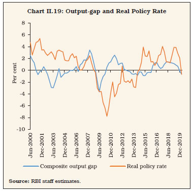 II.55 Empirical estimates suggest that for a one percentage point reduction in the real policy interest rate, the investment rate could increase by about 9 bps in the short-run and 109 bps in the long-run23. Reducing the real policy rate involves, however, tolerance of inflation up to 1 percentage point above target that can dampen investment by about 6 bps in the short-run and 69 bps in the long-run. A one percentage point reduction in the real policy rate enhances growth by 40 bps in the short-run and 52 bps in the long-run24. Tolerating higher inflation, however, involves sacrifice of growth by about 30 bps in the short-run and 40 bps in the long-run. On a net basis (using two comparable standardised parameters), GDP growth could increase by about 12 bps in the long-run, but this does not take into account the feedback from inflation to inflation expectations, and then to investment and growth. II.56 In order to incorporate this feedback loop, the QPM is employed25. The results show that a passive tolerance of higher inflation by one percentage point leads to unhinging of inflation expectations by a similar magnitude. This leads to decline in the real interest rate in the short-run, opening up a positive output gap. Inflation expectations settle at an elevated level over time, thereby, pushing up all the nominal variables, including the policy interest rate. This increase in the policy rate leads to an increase in the real interest rate later. The output gap closes to zero and real output returns to equilibrium leading to no long-term stimulating impact of higher inflation tolerance on GDP growth (Chart II.20). II.57 Trend GDP growth during the FIT period (pre-COVID) works out to 6.5 per cent26 when CPI headline inflation averaged 3.9 per cent. While presenting the Union Budget for 2019-20 in July 2019, the Honourable Union Finance Minister emphasised the need for directing policy priority for achieving the Honourable Prime Minister’s vision of a US$ 5 trillion size economy by 2024-25. Achieving this vision is feasible, as India has demonstrated in the past its capacity to deliver real GDP growth of 7.4 per cent during 2003-04 to 2010-11 and 2014-15 to 2018-19 (Table II.8). This would, however, require raising the investment rate in the economy so that it contributes 60 per cent of average GDP growth, supported by robust growth in capital formation (10.6 per cent per annum) and boosting exports (22 per cent growth per annum), as was the case during 2003-04 to 2010- 11. Total factor productivity has to contribute about 50 per cent to growth, on par with the 2014-15 to 2018-19 experience, supported by structural reforms (Annex II.5). 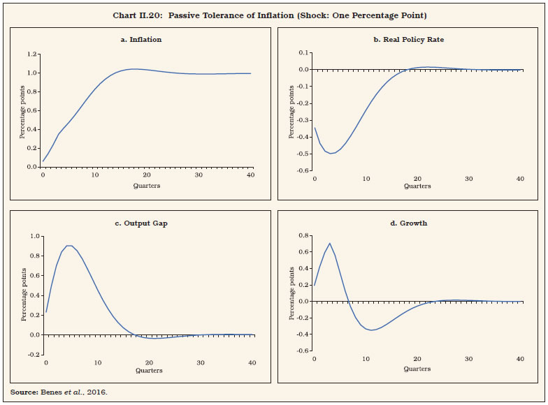
| Table II.8: Average GDP Growth and Related Indicators | | | 2003-04 to 2010-11 (per cent) | 2014-15 to 2018-19 (per cent) | | Real GDP growth | 7.4 | 7.4 | | Contribution from: | | | | Labour | 7.2 | -1.3 | | Capital | 60.1 | 43.5 | | Labour quality | 4.6 | 2.0 | | Capital quality | 4.0 | 5.0 | | Total factor productivity | 24.2 | 50.9 | | Nominal GDP growth | 15.0 | 11.0 | | US$ denominated GDP growth | 15.9 | 7.9 | | Share of gross capital formation in GDP | 36.6 | 32.8 | | Growth in gross fixed capital formation in GDP | 10.6 | 7.1 | | Growth of exports of goods and services | 22.3 | 6.0 | | Bank credit growth | 25.0 | 7.4 | | Share of NPAs (as proportion of advances) | 3.5 | 8.4 | | GDP deflator inflation# | 7.2 | 3.3 | | WPI inflation | 6.2 | 1.3 | | CPI-C inflation* | 7.1 | 4.5 | #: Compound annual growth rate for the entire period.
*CPI-IW for 2003-11 period.
Sources: KLEMS, RBI and NSO. | 7. Conclusion II.58 The international experience suggests that inflation targeting EMEs have either lowered their inflation targets or kept their targets unchanged over time. In India, however, the repetitive incidence of supply shocks, still elevated inflation expectations and projection errors necessitate persevering with the current numerical framework for the target and tolerance band for inflation for the next five years. II.59 The experience of advanced economies has shown that the zero lower bound is not particularly binding and the consequent loss of the interest rate as an instrument of monetary policy has led to a preponderant reliance of central banks on balance sheet policies which tend to inflate financial asset prices without any perceptible impact on the real economy. Meanwhile, structural changes in the economy, in particular demography, income distribution and falling trend growth are challenging the relevance of monetary policy as an instrument of stabilisation even as rising protectionism, digitisation, and climate change pose new risks. The pandemic is expected to leave permanent scars on the global economy, amplifying the effects of underlying structural changes and posing the risk of short-run disequilibria in the form of surges of inflation and increase in inequality. It is in this context that several central banks around the world are undertaking introspective reviews of their monetary policy frameworks and India cannot be immune to these tectonic shifts. Monetary policy has entered a twilight zone and until clarity emerges on the shape of the future, it is important to entrench its nominal anchor so that it can continue to perform its stabilising role. II.60 On the lower tolerance limit for the inflation target, measurement errors warrant caution. Since inflation targets in AEs remain unchanged at about 2 per cent, notwithstanding persistent deflationary conditions, the lower tolerance band in India should not be less than 2 per cent. This is also consistent with estimates of supply shocks presented in the chapter. On the upper tolerance limit, international experience suggests that countries with a large share of food in the CPI basket tend to have higher inflation targets and wider tolerance bands. Threshold estimates over a longer sample period work out to 6 per cent, beyond which tolerance of inflation can be harmful to growth. Hence, the current tolerance band of +/-2 per cent may be retained notwithstanding the central tendency emerging from the country experience of lowering targets and narrowing bands over time. References Agarwala, R. (2020), “India’s Inflation Targeting Framework Needs a Relook”. Business Line. Retrieved from https://www.thehindubusinessline.com/opinion/indias-inflation-targeting-provisions-need-a-relook/article32886547.ece Angeloni, I., Aucremanne, L., Ehrmann, M., Gali, J., Levin, A., and Smets, F. (2006), “New Evidence on Inflation Persistence and Price Stickiness in the Euro Area: Implications for Macro Modeling”, Journal of the European Economic Association, Vol. 4(2–3), 562–574. Ascari, G., and Sbordone, A. M. (2014), “The Macroeconomics of Trend Inflation”, Journal of Economic Literature, Vol. 52(3), 679–739. Bangko Sentral ng Pilipinas (2019), “Inflation Report”, BSP, Manila, Philippines. Behera, J., and Mishra, A. K. (2017), “The Recent Inflation Crisis and Long-run Economic Growth in India: An Empirical Survey of Threshold Level of Inflation”, South Asian Journal of Macroeconomics and Public Finance, Vol. 6(1), 105-132. Behera, H. K., and Patra, M. D. (2020), “Measuring Trend Inflation in India”, RBI Working Paper Series No. 15. Benes, J., K. Clinton, A. George, P. Gupta, J. John, O. Kamenik, D. Laxton, P. Mitra, G. Nadhanael, R. Portillo, H. Wang, and F. Zhang (2016), “Quarterly Projection Model for India: Key Elements and Properties”, RBI Working Paper Series No. 08. Bernanke, B. S. (2010), “Monetary Policy and the Housing Bubble”, A speech at the Annual Meeting of the American Economic Association, Atlanta, Georgia, January 3, 2010. Bhalla, S.S. (2017), “What ails GDP Growth in India – Demonetization or High Interest Rates?”, In Lensink, R., S. Sjögren and C. Wihlborg, Paths for Sustainable Economic Development, L,SandW, Gothenburg, Sweden, 265-272. Bhanumurthy, N. R., and Alex, D. (2008), “Threshold Level of Inflation for India”, Institute of Economic Growth Discussion Paper Series No. 124/2008, New Delhi: University Enclave. Bhattacharya, P., Kwatra, N., and Devulapalli, S. (2020), “Did Inflation-targeting Kill India’s Growth Story?”, The Livemint. Retrieved from https://www.livemint.com/news/india/did-inflation-targeting-kill-india-s-growth-story-11599461227389.html Bhoi, B.B., Kundu, S., Kishore, V., and Suganthi, D. (2019), “Supply Chain Dynamics and Food Inflation in India”, RBI Bulletin, Vol. 73(10), 95-112. Bratsiotis, G. J., Madsen, J., and Martin, C. (2002), “Inflation Targeting and Inflation Persistence”, Centre for Growth and Business Cycle Research Discussion Paper Series 211, Economics, The Univerisity of Manchester. Ciżkowicz-Pękała, M., Grostal, W., Niedźwiedzińska, J., Skrzeszewska-Paczek, E., Stawasz-Grabowska, E., Wesołowski, G., and Żuk, P. (2019), “Three Decades of Inflation Targeting”, NBP Working Paper No. 314, Narodowy Bank Polski. Clark, T. E., and Doh, T. (2014), “Evaluating Alternative Models of Trend Inflation”, International Journal of Forecasting, Vol. 30(3), 426–448. Cogley, T., Primiceri, G. E., and Sargent, T. J. (2010), “Inflation-gap Persistence in the US”, American Economic Journal: Macroeconomics, Vol. 2(1), 43–69. Dhanya, V., Shukla, A. K. , and Kumar, R. (2020), “Food Processing Industry in India: Challenges and Potential”, RBI Bulletin, Vol. 74(3), 27–41. Dholakia, R.H. (2020), “A Theory of Growth and Threshold Inflation with Estimates”, Journal of Quantitative Economics, Vol. 18(3), 471-493. Eichengreen, B., Gupta, P., and Choudhary, R. (2020), “Inflation Targeting in India: An Interim Assessment”, Policy Research Working Papers, The World Bank. Garga, V., and Singh, S. R. (2021), “Output Hysteresis and Optimal Monetary Policy”, Journal of Monetary Economics, Vol. 117, 871-886. Gerlach, S., and Tillmann, P. (2011), “Inflation Targeting and Inflation Persistence in Asia-Pacific”, Diambil Dari Hong Kong Institute for Monetary. Government of India (2018), “Economic Survey 2018-19”. IMF. (2013), “IMF Country Report No. 13/37: India Article IV Consultation”, International Monetary Fund, Washington D.C., USA. Jagannathan, R. (2019), “Scrap RBI’s Monetary Policy Panel or Give It A Dual Mandate”, The Livemint. Retrieved from: https://www.livemint.com/opinion/columns/opinion-the-mpc-should-be-scrapped-or-else-given-a-dual-mandate-1560852518727.html Jordà, Ò., Singh, S. R., and Taylor, A. M. (2020), “The Long-run Effects of Monetary Policy”, NBER Working Paper. No.26666. Kannan, R., and Joshi, H. (1998), “Growth-inflation Trade-off: Empirical Estimation of Threshold Rate of Inflation for India”, Economic and Political Weekly, 2724-2728. Khan, M. S., Senhadji, A., and Smith, B. D. (2001), “Inflation and Financial Depth”, IMF Working Paper – 01/44. Lacker, J. (2014), “Can Monetary Policy Affect Economic Growth”, Speeech at Johns Hopkins Carey Business School, Baltimore, Maryland. Libanio, G. (2010), “A Note on Inflation Targeting and Economic Growth in Brazil”, Brazilian Journal of Political Economy. Vol. 30, 73-88. Mallick, A., and Sethi, N. (2018), “What Causes India’s High Inflation? A Threshold Structural Vector Autoregression Analysis”, Institutions and Economies, 23-43. Meyer, L. H. (2001), “Inflation Targets and Inflation Targeting”, Federal Reserve Bank of St. Louis Review, Vol. 83(2001). Miyajima, K., and Yetman, J. (2018), “Assessing Inflation Expectations Anchoring for Heterogeneous Agents: Analysts, Businesses and Trade Unions”, BIS Working Papers 759, Bank for International Settlements. Mohaddes, M. K., and Raissi, M. M. (2014), “Does Inflation Slow Long-Run Growth in India?”, IMF Working Paper 14/222. Mohanty, D., Chakraborty, A. B., Das, A., and John, J. (2011), “Inflation Threshold in India: An Empirical Investigation”, Reserve Bank of India Working Paper Series, (18/2011). Nakajima, J. (2011), “Time-varying Parameter VAR Model with Stochastic Volatility: An Overview of Methodology and Empirical Applications”, Monetary and Economic Studies, November, 107-142. Okun, A. M. (1962), “Potential GNP: Its Measurement and Significance”, Yale University, Cowles Foundation for Research in Economics New Haven. Panagariya, A. (2015), “Retail Inflation Target Under MPF Could Be Revisited”, The Financial Express, Retrieved from https://www.financialexpress.com/economy/retail-inflation-target-under-mpf-could-be-revisited-arvind-panagariya/180520/ Papademos, L. (2003), “The Contribution of Monetary Policy to Economic Growth”, 31st Economic Conference. Vienna,12. Patra, M. D., Khundrakpam, J. K., and George, A. T. (2014), “Post-global Crisis Inflation Dynamics in India: What Has Changed”, India Policy Forum, Vol. 10(1), 117–203. Pattanaik, S., and Nadhanael, G. V. (2013), “Why Persistent High Inflation Impedes Growth? An Empirical Assessment of Threshold Level of Inflation for India”, Macroeconomics and Finance in Emerging Market Economies, Vol. 6(2), 204-220. Pattanaik, S., Behera, H. K., Kavediya, R., and Shrivastava, A. (2020), “Investment Slowdown in India: An Assessment”, Macroeconomics and Finance in Emerging Market Economies, DOI: 10.1080/17520843.2020.1865650. Phillips, A. W. (1958), “The Relation Between Un-employment and the Rate of Change of Money Wage Rates in the United Kingdom, 1861-1957”, Economica, Vol. 25(100), 283–299. Rangarajan, C. (1997), “Role of Monetary Policy”, Economic and Political Weekly, 3325–3328. Rangarajan, C. (1998), “Development, Inflation and Monetary Policy”, in I. Ahluwalia, and I. Little, India’s Economic Reforms and Development: Essays for Manmohan Singh, New Delhi: OUP. Rangarajan, C. (2020), “The New Monetary Policy Framework-What it Means”, Journal of Quantitative Economics, Vol. 18 (2), 457-470. RBI. (1985), “Report of the Committee to Review the Working of the Monetary System (Chairman: Sukhamoy Chakravarty)”, Reserve Bank of India. RBI (2002), “Report on Currency and Finance, 2001-02”, Reserve Bank of India, Mumbai. RBI (2011), “Annual Report, 2010-11”, Reserve Bank of India, Mumbai. RBI. (2014), “Report of the Expert Committee to Revise and Strengthen the Monetary Policy Framework (Chairman: Urjit R. Patel)”, Reserve Bank of India. Samantaraya, A., and Prasad, A. (2001), “Growth and Inflation in India: Detecting the Threshold Level”, Asian Economic Review, Vol. 43(3), 414-20. Sarel, M. (1996), “Nonlinear Effects of Inflation on Economic Growth”, Staff Papers, Vol. 43(1), 199– 215. Singh, K., and Kalirajan, K. (2003), “The Inflation-growth Nexus in India: An Empirical Analysis”, Journal of Policy Modeling, Vol. 25(4), 377-396. Singh, P. (2010), “Searching Threshold Inflation for India”, Economics Bulletin, Vol. 30(4), 3209-3220. Singh, C. (2014), “Inflation Targeting in India: Select Issues”, IIM Bangalore Research Paper No. 475. Smets, F., and Wouters, R. (2007), “Shocks and Frictions in US Business Cycles: A Bayesian DSGE Approach”, American Economic Review, Vol. 97(3), 586-606. Srinivasan, T. N. (2014), “Inflation Targeting Irrelevant in Indian Context”, The Economic Times. Retrieved from https://m.economictimes.com/news/economy/policy/inflation-targeting-irrelevant-in-indian-context-economist-t-n-srinivasan/articleshow/32437231.cms Stock, J. H., and Watson, M. W. (2007), “Why Has US Inflation Become Harder to Forecast?”, Journal of Money, Credit and Banking, Vol. 39, 3–33. Stock, J. H., and Watson, M. W. (2016), “Core Inflation and Trend Inflation”, Review of Economics and Statistics, Vol. 98(4), 770–784. Svensson, L. E. O. (1997), “Inflation Forecast Targeting: Implementing and Monitoring Inflation Targets”, European Economic Review, Vol. 41(6), 1111–1146. Tulasi, G., Samantaraya, A., Rajeshwar, T., and Chaubey, A. (2021), “Understanding Inflation Dynamics in India: A Revisit”, Economic & Political Weekly, Vol. 56 (2) pp. 42-50. Vasudevan, A., Bhoi, B. K., and Dhal, S. C. (1998), “Inflation Rate and Optimal Growth: Is There A Gateway to Nirvana”, Fifty Years of Developmental Economics: Essays in Honour of Prof. Brahmananda, 50-67.
Annex II.1: Threshold Inflation Estimates for India in Empirical Literature | Study | Period | Inflation Threshold
(per cent) | | Chakravarty Committee Report (1985) | | 4 | | Rangarajan (1998) | | 6 | | Kannan and Joshi (1998) | 1981-1995 | 6 | | Vasudevan, Bhoi and Dhal (1998) | 1961-1998 | 5-7 | | Samantaraya and Prasad (2001) | 1970-1999 | 6.5 | | Report on Currency and Finance (2002) | 1971-2000 | 5 | | Singh and Kalirajan (2003) | 1971-1998 | No Threshold (negative relation between growth and inflation) | | Bhanumurthy and Alex (2010) | 1976-2004/1997Q1-2005Q4/Jan2000-Apr2007 | 4-4.5 | | Singh (2010) | 1970-2009 | 6 | | RBI Annual Report 2010-11 | | 4-6 | | Pattanaik and Nadhanael (2013) | 1972-2011 | 6 | | Mohanty et al. (2011) | 1996-2011 | 4-5.5 | | IMF(2013) | 1996-2011 (Quarterly) | 5-6 | | RBI (2014) | 1997-2013 | 6.2-6.7 (CPI-C)
4.6-5.8 (WPI) | | Mohaddes and Raissi (2014) | 1989-2013 | 5.5 | | Behera and Mishra (2017) | 1990-2013 | 4 | | Mallick and Sethi (2018) | April 2006 to May 2015 | 4.8 | | Dholakia (2020) | 1995-96 to 2018-19 | 5.4 - 6 | | Rangarajan (2020) | 1982-2009 / 1992-2018 | 6-7 |
Annex II.2: Optimal Inflation in a Macroeconomic Framework In order to assess the optimal level of inflation of India using macro theoretic approach, a new class of “agent-based model (ABM)” is used where the interactions of heterogenous economic agents (e.g., households, firms, central bank and government) give rise to various macroeconomic outcomes and their decisions are not governed completely by rationality. ABMs can incorporate supply-demand mismatches and hence can be used to study adjustment mechanisms towards equilibrium. In the model (Gualdi et al., 2017), households’ consumption expenditure, which depends on their accumulated earnings and prices of consumable products, conditions the demand side of the economy. On the supply side, firms make adjustment to their production, price (of the product) and wage (offered to the labour) based on a host of factors which include profit, demand, credit and labour market conditions. The financial side of the economy is captured through commercial banks and their role in intermediation between savers (households) and borrowers (firms). The central bank sets the policy rate as per a Taylor-type rule to steer the inflation towards the target. The inflation target influences inflation expectations, which in turn affect the nominal prices and wages, real cost of credit faced by firms, and return on household savings, etc. The extent to which inflation target affects inflation expectations of the economic agents is governed by the credibility of the central bank. To determine the optimal level of inflation, the model is run multiple times with different values of inflation target ranging from zero to eight per cent. Each level of inflation target is associated with some benefits and costs, summarised in the form of output loss and price dispersion (Chart 1). The results imply an increase in output loss for inflation below 3.5 per cent and above 4.5 per cent and the loss is significantly high for inflation below 3 per cent. The price dispersion is found to increase with levels of inflation, and the increase is sharp for inflation above 5 per cent. The inflation reaches its optimal level when both output loss and price dispersion are at the lowest level. Therefore, a weighted measure of net cost/ benefit, combining both output loss and price dispersion is estimated through a loss function where equal weights are assigned for output variability and price dispersion. Optimal inflation is the level of inflation at which this loss function is minimised. The results show the loss is at its minimum level when the inflation is around 5 per cent (Chart 2). Further, the response of the loss function at a particular target level to varying degree of central bank credibility is assessed. The broad idea is that agents in the economy form inflation expectations based on actual inflation and the target. If the central bank is more credible, agents place more weight on the target and vice-versa. The results imply that improvement in the credibility of the central bank lowers the loss associated with a given level of the target. Reference Gualdi, S., Tarzia, M., Zamponi, F., and Bouchaud, J. P. (2017), “Monetary Policy and Dark corners in a Stylized Agent-based Model”, Journal of Economic Interaction and Coordination, 12(3), 507-537.
Annex II.3: Supply Shocks and the Lower Tolerance Band A standard medium-scale DSGE model (Smets and Wouters, 2007) is used to assess the impact of supply shocks on inflation. The model has three major blocks: households, firms and the government. The government block includes the fiscal and monetary authorities. The households are inter-temporal utility maximisers. They supply labour and capital to the firm sector in return of wage and rental earnings. They can save either in risk-free one period government bond or in capital. They also choose how intensively capital is used in the production process. Their decision about how much to save in capital determines the investment level in the economy. The firm sector includes two types of firm, viz. a final-goods producing firm and a continuum of intermediate goods producing firms. The production function of intermediate-goods producing firms combine labour and capital according to the constant returns to scale (CRS) technology. The final-goods firm combines the produce of intermediate-firms according to standard Dixit- Stiglitz aggregation, which is then sold to the households. The fiscal authority issues bonds and raises lump-sum taxes to meet the expenditure on goods and services. The monetary authority sets the nominal interest rate following a Taylor-type rule. The interest rate affects the economy by influencing the behaviour of optimising households broadly in two ways: first, it affects inter-temporal substitution between consumption and savings and, second, it also influences the intra-temporal substitution between bond and capital investment. Identification of supply shocks The intermediate firms operate in a monopolistically competitive environment and hence possess pricing power. However, they are assumed to face Calvo (1983) type price rigidity, which results in to the following New Keynesian hybrid Phillips curve specification, Here ɑ, b and c are the appropriate reduced form coefficients capturing the impact of lagged inflation, forward-looking inflation expectations and real marginal cost, respectively, on actual inflation. The shock term captures the residual impact on inflation excluding the demand side effects originating from households and the government. This acts as a reduced-form proxy capturing the effect of supply-side shocks on inflation. References: Calvo, G. A. (1983), “Staggered Prices in a Utility- Maximizing Framework”, Journal of Monetary Economics, Vol. 12(3), 383-398. Smets, F., and Wouters, R. (2007), “Shocks and Frictions in US Business Cycles: A Bayesian DSGE Approach”, American Economic Review, Vol. 97(3), 586-606.
Annex II.4: Objectives of Monetary Policy for the Inflation Targeting Countries | Sr. No. | Country | Year of Adoption of IT | Key Monetary Policy Objective | | Countries with single mandate of Inflation targeting | | 1 | Brazil | 1999 | “Keeping inflation around the target is a fundamental objective of the Banco Central do Brasil (BCB).” | | 2 | Japan | 2013 | The Bank of Japan Act states that the Bank's monetary policy should be “aimed at achieving price stability.” | | 3 | Switzerland | 2000 | “…ensure price stability.” | | 4 | Chile | 1999 | “…the primary objective of monetary policy is price stability.” | | 5 | Czech Republic | 1997 | “… primary purpose is to maintain price stability.” | | 6 | Sweden | 1993 | “... maintain price stability.” | | 7 | Mexico | 2001 | “...its primary objective shall be to seek the stability of the purchasing power of said currency.” | | 8 | Russia | 2015 | “The objective of monetary policy is “to ensure price stability, that is, sustainably low inflation.” | | 9 | Egypt | 2005 | “...price stability being the primary and overriding objective.” | | 10 | Iceland | 2001 | “The principal objective of the Central Bank of Iceland is to promote price stability.” | | 11 | Armenia | 2006 | “The primary goal of the CBA is prices stability.” | | 12 | Canada | 1991 | “to preserve the value of money by keeping inflation low, stable and predictable.” | | 13 | Poland | 1998 | “The basic objective of the activity of NBP shall be to maintain price stability, while supporting the economic policy of the Government, insofar as this does not constrain the pursuit of the basic objective of NBP.” | | 14 | Kazakhstan | 2015 | “... ensuring price stability in the Republic of Kazakhstan.” |
| Sr. No. | Country | Year of Adoption of IT | Key Monetary Policy Objective | | Countries with Dual/multiple mandates | | 1 | Australia | 1993 | “…the Reserve Bank Board will best contribute to the stability of the currency of Australia, the maintenance of full employment, and the economic prosperity and welfare of the people of Australia.” | | 2 | New Zealand | 1990 | “The objective of monetary policy is to achieve “the economic objectives of price stability” and support “maximum sustainable employment.” | | 3 | USA | 2012 | “…so as to promote effectively the goals of maximum employment, stable prices, and moderate long-term interest rates.” | | 4 | UK | 1992 | “to maintain price stability and subject to that, to support the economic policy of Her Majesty’s Government, including its objectives for growth and employment.” | | 5 | Turkey | 2006 | “The Bank shall, provided that it shall not conflict with the objective of achieving and maintaining price stability, support the growth and employment policies of the Government.” | | 6 | Colombia | 1999 | “The objective of monetary policy in Colombia “is to keep inflation low and stable and to achieve the highest sustainable level of output and employment.” | | 7 | Israel | 1997 | “…to maintain price stability as its central goal.”
“…to support other objectives of the Government’s economic policy, especially growth, employment and reducing social gaps… this support shall not prejudice the attainment of Price Stability over the Course of Time.” | | 8 | Thailand | 2000 | “conducts monetary policy under a flexible inflation targeting framework, putting emphasis on achieving price stability alongside preserving economic growth and financial stability.” | | 9 | South Korea | 2001 | “…by pursuing price stability through the formulation and implementation of efficient monetary and credit policies.”
“…the Bank of Korea shall pay attention to financial stability in carrying out its monetary and credit policies.” | | 10 | Indonesia | 2005 | “Exchange rate stability along with price stability” | | 11 | ECB | 2003 | “To maintain price stability is the primary objective of the Eurosystem.”
“Without prejudice to the objective of price stability... achievement of the objectives of the Union. These include inter alia “full employment” and “balanced economic growth.” | | 12 | Norway | 2001 | “the primary objective of monetary policy is low and stable inflation.”
“Inflation targeting shall be forward-looking and flexible so that it can contribute to high and stable output and employment, and to counteracting financial imbalances.” | | 13 | Ghana | 2007 | “In addition to price stability, the Bank is enjoined to support the general economic policy of Government, promote economic growth and development, and ensure effective and efficient operation of the banking and credit system; and contribute to the promotion and maintenance of financial stability.” | | 14 | Philippines | 2002 | “The primary objective of the BSP's monetary policy is to promote a low and stable inflation conducive to a balanced and sustainable economic growth. It shall also promote and maintain monetary stability and the convertibility of the peso.” | | 15 | Ukraine | 2016 | The Law of Ukraine On the National Bank of Ukraine identifies a priority list of objectives for the NBU in the following order:
1. “...the primary objective of the NBU is to ensure stability of the monetary unit of Ukraine.”
2. “...achievement and maintenance of price stability.”
3. “...shall promote... financial stability, including stability of the banking system, without prejudice of the objective set forth in the second part.”
4. “…shall also promote sustainability of the economic growth and support the economic policy of the Cabinet of Ministers of Ukraine provided that it does not prevent the NBU from attainment of the aims determined in the second and third parts of this Article.” |
Annex II.5: Structural Reforms during Inflation Targeting Regime | Reform Measures | Actual/Likely Outcome | | Insolvency and Bankruptcy Code (IBC), 2016 | Time-bound resolution of stressed assets. According to the World Bank Doing Business Report, 2020, the time taken to resolve stressed loans declined from 4.3 years to 1.6 years, while recovery rate improved from 26 per cent to 72 per cent, four years into IBC. | | Goods and Services Tax Act, 2017 | To simplify the indirect tax regime, create a common national market by subsuming a myriad of Central and State taxes, and reducing the incidence of tax-on-tax.
India witnessed a fall in the weighted average effective GST rate from 14.4 per cent to 11.6 per cent in 2019. | | Real Estate (Regulation and Development) Act, 2016 | Imparted transparency and boosted home buyers’ sentiment. | | Labour Reforms | Rationalisation of labour laws to enhance ease of doing business and improve employment opportunities by promoting a flexible labour market along with widening access to social security. | | MSMEs: Turnover as an additional criterion | Increased compatibility of new definition with GST data will help streamline access to information for lenders. | | Commercial Mining of Coal open to private sector participation. | Aims at reducing import of coal and increase self-reliance in coal production. | | Privatisation of Public Sector Enterprise | Aims to privatise PSEs, except the ones functioning in certain strategic sectors which has been notified by the government. In strategic sectors, bare minimum PSEs will remain, but private sector will also be allowed. | | Model Agriculture and Land Leasing Act 2016 | Increased land use efficiency and income for landless farmers. | | Essential Commodities Act, 1955 amendment (June 2020) | To attract fresh investments and create a seamless market and better value for farm produce. | | Farmers (Empowerment and Protection) Agreement on Price Assurance and Farm Services Act, 2020 | Create assured markets for farmers and quality raw materials for industry. | | The Farmers’ Produce Trade and Commerce (Promotion and Facilitation) Ordinance 2020 | Opportunity for private sector to set up private markets, alternative marketing channels and online market platforms. | | Early Recognition, Adequate Provisioning and timely resolution of stressed assets | Asset quality review (AQR) ensured realistic assessment of asset quality of SCBs.
Provision coverage ratio of banks (without write-off adjusted) rose from 41.7 per cent at end-March 2015 to 66.2 per cent at end-March 2020. RBI circular of June 7, 2019 - strong disincentives via additional provisions for delay in initiating resolution process. | | Mergers and privatisation of banks and insurance companies | Merger of public sector banks (PSBs) to create next generation banks that have strong local as well as global presence.
In June 2020, there were 12 PSBs as against 27 PSBs at end March 2019.
Privatisation of two PSBs and one general insurance company in 2021-22 has been proposed in the Union Budget. | | Banking Governance Reforms | Bank Board Bureau formed; guidelines on incentive structure of top management in private sector banks issued. | | Taxation Laws (Amendment) Act, 2019 | Effective tax rate for domestic corporates, inclusive of surcharges, to decline from 34.94 per cent to 25.17 per cent if other tax sops are not availed.
For new manufacturing firms set up after October 1, 2019 and commencing operations by March 31, 2023, the effective tax rate will fall from 29.1per cent to 17per cent.
Measures introduced to boost investments and increase the productive capacity of the economy. | | Production Linked Incentive (PLI) Scheme | Scheme worth ₹1.97 lakh crore for 13 key sectors with the objective to create manufacturing global champions. This initiative will help bring scale and size in key sectors, create and nurture global champions and provide jobs to our youth. | | Survey of Villages Abadi and Mapping with Improvised Technology in Village Areas (SVAMITVA) scheme | Aims to reduce property litigations and transaction costs and improve the ease of doing business by bringing clarity in land ownership. | | National Monetisation Pipeline | Monetising operating public infrastructure assets is a very important financing option for new infrastructure construction. A dedicated dashboard will create visibility among investors. |
| Bai-Perron Structural Break Tests | | Period | Intercept Coef. | t-Stat | | 1997Q2 - 2000Q2 | 7.64*** | 12.11 | | 2000Q3 - 2008Q1 | 4.62*** | 11.31 | | 2008Q2 - 2014Q2 | 9.90*** | 21.77 | | 2014Q3 - 2020Q1 | 4.39*** | 9.25 | | R2 | 0.53 | | | ***: Significant at less than 1 per cent level. | |