In the midst of global slowdown accentuated by the vicissitudes of financial markets and the transient impact of demonetisation, the Indian economy turned out resilient, marked by both internal and external stability. While economic growth moderated in 2016-17, there were visible signs of improvement in macroeconomic fundamentals – low inflation, and modest current account deficit and fiscal deficit. Going forward, even as the recent launch of the Goods and Services Tax (GST) gains traction across the country, strengthening fiscal consolidation, particularly at the sub-national level; reviving bank credit, and bringing investment back on rails, remain a challenge. II.1 The Real Economy II.1.1 Against the backdrop of activity and trade slowing across advanced and emerging economies, firming commodity prices and bouts of volatility interrupting generally rallying financial markets, the Indian economy posted a resilient performance in 2016-17, underpinned by macroeconomic stability. The provisional estimates of national accounts released by the Central Statistics Office (CSO) in May 2017 reveal that real Gross Value Added (GVA) growth moderated in 2016-17 from a year ago, mainly located in the services sector (Chart II.1a). Public administration, defence and other services (PADO) cushioned the slowdown, adding 2.2 percentage points to the growth of real GVA in the services sector and 1.4 percentage points to the growth of overall GVA of 6.6 per cent. GVA in mining and quarrying activities also decelerated sharply. However, mining output expanded as the narrative on aggregate supply in this section will show. 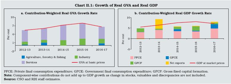 II.1.2 In contrast, agriculture and allied activities shrugged off the fetters of two consecutive monsoon failures and rebounded on the back of all-time highs in the production of foodgrains, fruits and vegetables. A key driver turned out to be pulses, profiled in Box II.2. Manufacturing slowed in relation to the preceding year but held up above trend. It was sustained by healthy revenues of manufacturing corporations, alongside an improvement in the output of the unorganised sector. Electricity generation and the supply of other utilities were boosted by the inclusion of renewable sources of energy in the new index of industrial production (IIP) as discussed in para II.1.16. II.1.3 Aggregate demand, which is featured in the immediately following sub-section, suffered from a sharp slowdown in gross capital formation as entrepreneurial energies flagged and a sluggish appetite for new investment took its toll on business confidence. As a consequence, gross fixed capital formation (GFCF) contributed barely 0.7 percentage point to the real GDP growth of 7.1 per cent in 2016-17 despite accounting for around one-third of real GDP (Chart II.1b). Net exports contributed 0.4 percentage point, helped by a turnaround in merchandise export performance after contraction in the previous year. The rest of the real GDP growth was consumption-driven - both private and public. In fact, absent the implementation of the 7th Central Pay Commission and one-rank-one-pension (OROP) for defence services embedded in government consumption, real GDP growth would have been lower by 2 percentage points. Private consumption spending alone contributed two-thirds of the growth of aggregate demand. In this context, Box II.1 addresses issues around the sustainability of consumption-led growth and its unintended consequences. Aggregate Demand II.1.4 The slackening of aggregate demand set in from the first quarter of the year. This is confirmed by the loss of momentum showing up in three-quarter moving averages of seasonally adjusted annualised growth rates (MA-SAARs) (Chart II.2). II.1.5 Underlying the loss of momentum, GFCF began to lose height from Q2 and sank into contraction in Q4 of 2016-17. This was mirrored in proximate coincident indicators – steel consumption and cement production (Chart II.3). This development is worrisome in view of the secular-like retreat of the rate of gross domestic investment in the 2011-12 based GDP series [incorporating the new indices of industrial production (IIP) and wholesale prices (WPI)] to 29.5 per cent of GDP in 2016-17. 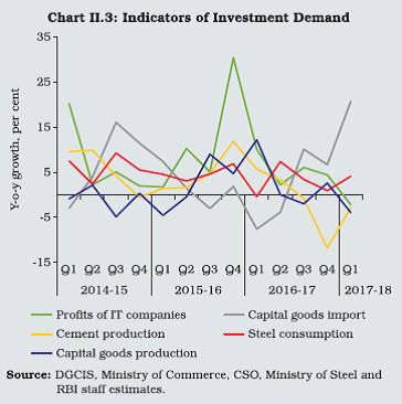 II.1.6 While the falling away of fixed investment mainly occurred in household dwellings, other buildings and structures (Chart II.4), the investment climate remained sombre. Fixed investment by other agents – government and private non-financial corporations – increased, but marginally, to provide an offset. The Reserve Bank’s survey of order books, inventories and capacity utilisation indicated persisting slack in capacity utilisation (seasonally adjusted) in manufacturing in 2016- 17. The capacity utilisation was observed to co-move closely with the de-trended industrial production. New investment intentions contracted in 2016-17 with respect to both government and private sectors, with the cost of private projects remaining elevated (Chart II.5a). Plant load factors in thermal power plants underwent a sustained decline, largely reflecting weakness in demand from financially stressed distribution companies. 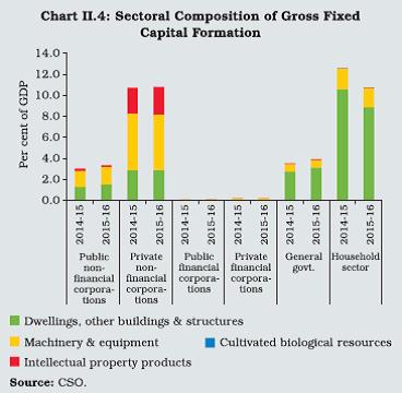
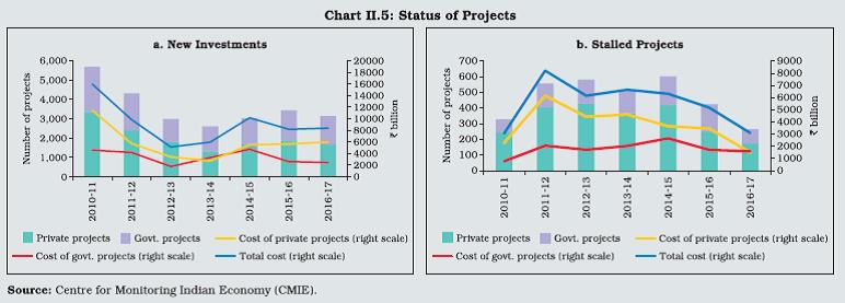 II.1.7 The resilience of some infrastructure sectors in the face of this downturn is noteworthy and brightens the outlook. First, there was a decline in cost and time overruns in central sector infrastructure projects (₹1.5 billion and above). Second, awarding and construction of highway projects in the road sector reached an all-time high even as daily additions to the roads constructed touched a peak of 22.6 km during 2016-17 from 16.6 km last year. Third, stalled projects declined by 40 per cent in terms of value and 37 per cent in terms of number (Chart II.5b). Fourth, capacity addition in major ports was the highest ever in a single year and 12 major ports recorded higher growth in cargo traffic as well as efficiency gains measured in turnaround time (3.43 days in 2016- 17 as against 3.64 days in the previous year), and average output per ship berth day (14,576 tonnes in 2016-17 as against 13,748 tonnes in the previous year). II.1.8 In the power sector, 27 states/UTs joined the Ujwal DISCOM Assurance Yojana (UDAY) to deleverage and revive distribution companies, and issued bonds worth ₹2.32 trillion (86.3 per cent of the target of ₹2.69 trillion). In the civil aviation sector, a Regional Connectivity Scheme (RCS) was launched in October 2016. In the automobile sector, the government provided incentives for demand and manufacture of electric/hybrid vehicles. In matters of government procurements, a new policy decision has been taken in favour of domestically manufactured goods. II.1.9 Consumption expenditure set a floor to the slowdown in real GDP growth in 2016- 17 and actually accelerated in the second half of the year when the impact of demonetisation was the most intense. This proved fortuitous as it coincided with the deepening retrenchment in fixed investment. Government final consumption, boosted by revisions in salaries and pensions referred to earlier, provided nearly a third of this support. Private consumption expenditure also benefited from rising real incomes – from the sharp fall in inflation and crowding-in income effects of government spending – and raised its contribution to real GDP growth from 57 per cent in H1 of 2016-17 to about 79 per cent in H2. The strength of private consumption was reflected in the acceleration of agricultural GVA as well as the sizable increase in telephone connections, indirect tax collections and the index of manufacturing constituting a part of industrial production. Consumption as a driver of growth has been associated with low growth multipliers and ‘half-life’, with some evidence that side effects such as rising household indebtedness could turn out to be growth-retarding in the medium-term (Box II.1). Box II.1
Is Consumption-Led Expansion Sustainable?: A Case Study of India In recent years, GDP growth in India has been consumption-led, more so during 2013-14 and 2016-17 (Chart 1a). In such a phase of growth, consumption grows faster than GDP, either in nominal or real terms, so that the consumption-to-GDP ratio increases over time or alternatively, real consumption growth exceeds real GDP growth (Kharroubi and Kohlscheen 2017). Consumption-led growth can arguably lead to a slackening of future growth if it entails growing imbalances due to limits to capacity creation, and rising debt burdens, particularly for households. Evidently, while borrowings helped smoothen private consumption in the short-run after the recession of 2001-02, excessive leverage led to the debt-servicing burden which, in turn, debilitated consumption and overall growth during 2007 to 2009 in the U.S (Dynan 2012). 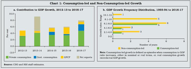 Private consumption contributes more than half of India’s GDP growth and is less volatile than other sources of expenditure. At a high growth level (above 8 per cent), the growth process was observed to be non-consumption-led (Chart 1b)1. Given that India has a large domestic consumer market, consumption may be the inevitable means of economic growth. However, whether consumption-led growth is beneficial for economic growth or acts as a drag remains to be assessed, particularly in view of the fact that rates of growth in investment and net exports have not been very impressive in recent years. Drawing on Kharroubi and Kohlscheen (2017), two issues were examined for the period 1993-94 to 2014-15: (i) whether consumption-led growth was associated with a subsequent slowdown in real GVA growth; and (ii) whether the debt burden of the household sector was a mechanism thereof. Growth in private (corporate plus household) credit to GDP ratio and growth in combined debt service ratio2 (interest payment to GDP ratio) for corporate and household sectors were included as control variables: Y is real GVA growth, CL is a variable counting the number of years of consumption-led growth between year t-3 and t, PC is growth in private credit-to-GDP, and DSR is growth in the debt service ratio in year t. In the next step, the impact of growth in household credit to GDP ratio and growth in the debt service ratio of the household sector, apart from the number of episodes of consumption-led growth in the preceding three years, on subsequent real consumption growth was estimated. Ct is real consumption growth, and HHC is growth in household credit-to-GDP, and DSRHH is growth in the debt service ratio of household in year t. Consumption-led growth was found to have a negative impact on GVA growth one-year ahead by 1.39 percentage points at 5 per cent significance level. The impact of the debt service ratio was significant neither numerically (-0.1 percentage point) nor statistically, indicating the muted role of formal finance in driving consumption growth. Consumption-led growth did have, albeit not statistically significant, a negative impact on consumption growth one-year ahead. These results corroborate the imperative for a judicious balance in the growth drivers for non-disruptive and sustainable long-term growth. References: 1. Dynan, K. (2012), “Is a Household Debt Overhang Holding Back Consumption?”, Brookings Papers on Economic Activity. 2. Kharroubi, E. and E. Kohlscheen (2017), “Consumption-led Expansions”, BIS Quarterly Review, March. | II.1.10 In terms of financing, household financial savings - the most important source of funds for investment in the economy - picked up to 7.8 per cent of Gross National Disposable Income (GNDI) in 2015-16 on the back of improvement in real income (Table II.1). Savings of private non-financial corporations increased to 10.8 per cent of GNDI in 2015-16. At the same time, general government’s dissaving declined to 1.0 per cent in 2015-16 (Appendix Table 3). On the investment front, households’ physical assets declined sharply to 10.7 per cent in 2015-16, contributing to the overall decline in fixed capital formation. The net inflow of resources from abroad to supplement domestic saving remained muted, mirrored in modest current account deficits as presented in Section II.6. As per preliminary estimates, household financial savings rate increased further to 8.1 per cent of GNDI in 2016-17 on account of an increase in households’ assets in bank deposits, life insurance and mutual funds, even though currency with the public contracted during the year. Higher financial savings were mainly supported by lower inflationary scenario as also portfolio adjustment from physical to financial assets by households. At the same time, there was an increase in financial liabilities of the household sector. | Table II.1: Financial Saving of the Household Sector | | (Per cent of GNDI) | | Item | 2011-12 | 2012-13 | 2013-14 | 2014-15 | 2015-16 | 2016-17* | | 1 | 2 | 3 | 4 | 5 | 6 | 7 | | A. Gross financial saving | 10.4 | 10.5 | 10.4 | 10.1 | 10.9 | 11.8 | | Of which: | | | | | | | | 1. Currency | 1.2 | 1.1 | 0.9 | 1.1 | 1.4 | -2.1 | | 2. Deposits | 6.0 | 6.0 | 5.8 | 5.0 | 4.8 | 7.3 | | 3. Shares and debentures | 0.2 | 0.2 | 0.2 | 0.2 | 0.3 | 1.2 | | 4. Claims on government | -0.2 | -0.1 | 0.2 | 0.0 | 0.5 | 0.5 | | 5. Insurance funds | 2.2 | 1.8 | 1.8 | 2.4 | 1.9 | 2.9 | | 6. Provident and pension funds | 1.1 | 1.5 | 1.5 | 1.5 | 2.0 | 1.9 | | B. Financial liabilities | 3.2 | 3.2 | 3.1 | 2.9 | 3.1 | 3.7 | | C. Net financial saving (A-B) | 7.2 | 7.2 | 7.2 | 7.2 | 7.8 | 8.1 | *: As per the latest estimates of the Reserve Bank; GNDI: Gross national disposable income.
Note: Figures may not add up to total due to rounding off.
Source: CSO. | Aggregate Supply II.1.11 On the supply side, GVA at basic prices – GDP stripped of net product taxes – also slowed quarter after quarter in 2016-17, the slump more pronounced in H2. MA-SAAR reveals this sharp loss of momentum (Chart II.2). II.1.12 The quarterly pattern of GVA growth tracked that of the services sector in which, too, the deceleration was stark in H2 and co-moving in all constituents, barring PADO. Although not as well synchronised, the evolution of the GVA of industry also dragged during H2, essentially in manufacturing (Table II.2). | Table II.2: Real GVA Growth (2011-12 Prices) | | (Per cent) | | Item | 2015-16 | 2016-17 | | Q1 | Q2 | Q3 | Q4 | Q1 | Q2 | Q3 | Q4 | | 1 | 2 | 3 | 4 | 5 | 6 | 7 | 8 | 9 | | I. Agriculture, forestry and fishing | 2.4 | 2.3 | -2.1 | 1.5 | 2.5 | 4.1 | 6.9 | 5.2 | | II. Industry | 7.7 | 9.2 | 12.0 | 11.9 | 9.0 | 6.5 | 7.2 | 5.5 | | i. Mining and quarrying | 8.3 | 12.2 | 11.7 | 10.5 | -0.9 | -1.3 | 1.9 | 6.4 | | ii. Manufacturing | 8.2 | 9.3 | 13.2 | 12.7 | 10.7 | 7.7 | 8.2 | 5.3 | | iii. Electricity, gas, water supply and other utility services | 2.8 | 5.7 | 4.0 | 7.6 | 10.3 | 5.1 | 7.4 | 6.1 | | III. Services | 8.9 | 9.0 | 9.0 | 9.4 | 8.2 | 7.4 | 6.4 | 5.7 | | i. Construction | 6.2 | 1.6 | 6.0 | 6.0 | 3.1 | 4.3 | 3.4 | -3.7 | | ii. Trade, hotels, transport, communication and services related to broadcasting | 10.3 | 8.3 | 10.1 | 12.8 | 8.9 | 7.7 | 8.3 | 6.5 | | iii. Financial, real estate and professional services | 10.1 | 13.0 | 10.5 | 9.0 | 9.4 | 7.0 | 3.3 | 2.2 | | iv. Public administration, defence and other services | 6.2 | 7.2 | 7.5 | 6.7 | 8.6 | 9.5 | 10.3 | 17.0 | | IV. GVA at basic prices | 7.6 | 8.2 | 7.3 | 8.7 | 7.6 | 6.8 | 6.7 | 5.6 | | Source: CSO. | II.1.13 GVA in agriculture and allied activities rose to recent peaks with every harvest arrival during the year and cushioned the impact of the downturn in other sectors. This strong revival occurred on the back of normal precipitation [97 per cent of the Long Period Average (LPA)] in the south-west monsoon (SWM). Out of 36 sub-divisions, 27 sub-divisions received normal/ excess rainfall. The initial delay in the monsoon’s onset was more than compensated by recovery in July-August 2016 and a belated departure. This helped maintain soil moisture and replenished reservoirs. Consequently, even though the north-east monsoon (NEM) ended at 45 per cent below LPA, the reservoir position remained above the 10-year average. At the end of December 2016, the water level in 91 major reservoirs across the country stood at 126 per cent of the live storage a year ago. Rabi sowing turned out to be higher by 5.7 per cent than in the previous year, aided by higher MSPs (especially for pulses) and availability of key agricultural inputs. II.1.14 The fourth advance estimates of crops for 2016-17 have placed the production of foodgrains at 275.7 million tonnes, which is 9.6 per cent higher than in the previous year and a historical record. Within foodgrains, rice, wheat, pulses and coarse cereals recorded their highest ever production levels. Besides favourable agro-climatic conditions, multi-pronged initiatives such as incentives for crop diversification, issuance of soil health cards, focus on integrated irrigation schemes, a simplified crop insurance scheme and improved marketing facilities created an enabling environment. The record production spurred an extensive drive to procure rice and wheat to replenish depleted stocks (Chart II.6). The all-time high production of pulses at 22.95 million tonnes, combined with a surge in imports of as much as 6.6 million tonnes, facilitated the build-up of buffer stock during the year (Box II.2). The production of horticulture increased by 3.1 per cent to 295.2 million tonnes, another record.  II.1.15 For 2017-18, the Ministry of Agriculture set higher targets of production for foodgrains (both cereals and pulses) as well as commercial crops (sugarcane, oilseeds and cotton). Early indications based on the progress of kharif sowing, and arrival of monsoon augur well for achieving the production targets. Region-wise, the distribution of rainfall during 2017-18 so far has, however, been somewhat uneven, with the east and north-east region receiving rainfall above LPA while the south peninsula (particularly Kerala and Karnataka) and the central India (particularly Madhya Pradesh) experiencing deficiency (Chart II.7). 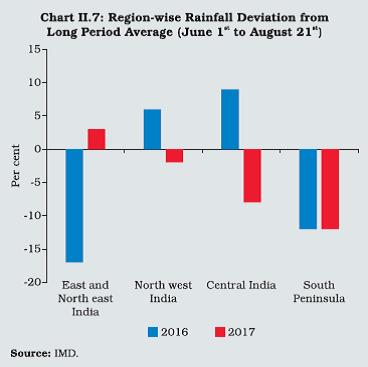 II.1.16 The deceleration in the growth of GVA in industry in 2016-17 in relation to the preceding year is not reflected in the new series of IIP. The CSO released a new series on the IIP in mid-May 2017, changing (a) the constituent items to better represent the evolving industrial structure; and (b) the base year to 2011-12 from 2004-05, thereby aligning it with national accounts and the new WPI. In terms of the new IIP, industrial production accelerated in 2016-17 across sectors. The wedge between industrial GVA and IIP mainly reflects the impact of falling input costs. Box II.2
Dynamics of Pulses Production In India, which is the largest producer, consumer and importer of pulses - a major plant source of protein - domestic demand follows the celebrated Bennett’s Law: the pattern of consumption shifts in favour of nutritious food as incomes rise. Low and near stagnant productivity, and excessive reliance on the monsoon are widely identified as the biggest impediments to augmenting domestic output (Chart 1.a & b). As a fallout, 15-20 per cent of the domestic requirement of pulses was made up by imports through the last 15 years (Chart 1.b).
Noting that the production of pulses seems to have linkages with the price support system, the role of prices of pulses as a determinant of production is examined in a dynamic panel generalised method of moments (GMM) framework, using data of 28 states for 2006-16:  The results indicate that much of the increase in production during the period was due to increased acreage though the impact of own lag was found to be insignificant statistically. Yield has a relatively subdued effect, albeit significant and positive in sign, possibly reflecting its low and stagnant level. Rainfall and MSP up to a year lag, that directly affect acreage, which also proxy for absence of adequate pulses irrigation (only 19.0 per cent of net sown area irrigated) and the prospect of remunerations (as MSP sets floor price), respectively, were statistically significant as instrumental variables. Prices and production of pulses share a positive relationship of statistical significance. The instrumental variables, viz., CPI with a one year lag, imports and input costs that have a bearing on current prices, also turned out significant. The significance of soyabean’s MSP – a competing crop for pulses - as an instrumental variable possibly indicates a shift in acreage across crops. Prices of pulses follow a cycle. Years of bumper production are preceded by monsoon failure, high pulses inflation, and their imports. Subsequently, farmers are incentivised by remunerative global and/or domestic prices coupled with higher than usual hikes in MSPs to bring in more areas under cultivation. Thereafter, prices of pulses generally crash when they arrive in the markets, which acts as a dis-incentive for production in the next season and causes pulses prices to rise again, akin to the Cobweb Model or Hog Cycle (alternatively called pork cycle or cattle cycle) based on production lags and adaptive expectations (Rosen, et al. 1994). The cycle has traversed the full distance from peak to peak, rendering pulses cultivation six times riskier than paddy (GoI 2016). Raising pulses production through integrated management (seeds, fertilisers, insecticides and pesticides) to improve yields, and weather proofing by expanding irrigation facilities, should be the Government’s strategy for the medium to long-term. In the interregnum, however, targeted use of remunerative MSPs – announced on time without delay in payment, coupled with predictable procurement operations as also providing vent in the form of export and futures trading to liquidate excess stocks, may be necessary safeguards against prices crashing during harvests so that production is sustained. References: 1. Government of India (2000), “Expert Committee Report on Pulses” (Chairman: Dr. R.S. Paroda). 2. _______ (2012), “Report of Expert Group on Pulses” (Chairman: Dr. Y. K. Alagh), DAC. 3. _______ (2016), “Incentivising Pulses Production Through Minimum Support Price (MSP) and Related Policies” (Chairman: Dr. Arvind Subramanian), September. 4. Rosen, S., K. Murphy and J. Scheinkman (1994), “Cattle Cycles”, Journal of Political Economy, 102 (3): 468-492. 5. The National Academy of Agricultural Sciences (2016), “Towards Pulses Self-Sufficiency in India”. 6. Thangzason, S., D. K. Raut, Pallavi and D. P. Rath, “What has Gone Wrong with Pulses?”, mimeo. | II.1.17 The new IIP has expanded the coverage of manufacturing sector from 620 items in 397 groups to 809 items in 405 groups. With the increase in item groups reporting in value terms from 53 to 109 (mostly in the capital goods category), capital goods now include ‘work-in-progress’ and thus account for longer production cycles and minimise the volatility resulting from bulk reporting on delivery. Other major changes in the manufacturing index include higher weightage to petroleum products (from 6.7 per cent to 11.8 per cent) to account for subsidies and inclusion of a new sub-group “Manufacture of pharmaceuticals, medicinal chemical and botanical products”. The new index excludes unorganised manufacturing while deciding on weights. Electricity index now captures electricity generation out of renewable sources while the number of minerals have been reduced from 62 to 29 in the mining index, taking into account the reclassification done by the Mineral Conservation and Development Rules, 2016. A new use-based category, ‘infrastructure/ construction goods’ has been introduced while ‘basic goods’ have been re-christened as ‘primary goods’. The weights of primary goods and consumer non-durables have declined on transfer of items to the infrastructure/construction category. The weight of manufacturing has increased while that of electricity has reduced in the overall index. A standing Technical Review Committee to be chaired by the Secretary, Ministry of Statistics and Programme Implementation (MoSPI), has been set up for an on-going revision of IIP. Based on the new index, industrial production recorded a compound annual growth of 3.8 per cent during 2012-13 through 2016-17 as against 1.2 per cent in the old index. In 2016-17, IIP increased by 4.4 per cent as against a contraction of 0.1 per cent under the old index (Chart II.8). 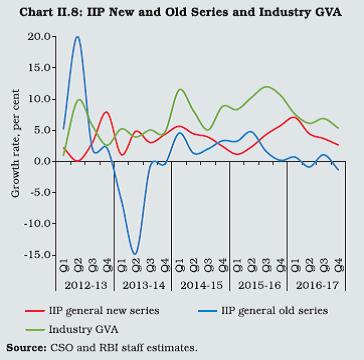 II.1.18 Structural bottlenecks became manifest in a persistent sluggishness in the production of crude oil and natural gas sub-sectors; yet, in spite of this drag, mining output accelerated, which was led by coal and refinery products. The manufacturing sector also gained speed over the year, particularly with respect to pharmaceuticals, motor vehicles, transport equipment, basic metals, petroleum products, wearing apparel, and machinery and equipment. Despite a moderation in the dominant thermal segment, the electricity sector managed a slight uptick on the back of renewable energy sources (Table II.3). Efforts are underway to financially turn around the electricity distribution companies (DISCOMs) through UDAY, as discussed earlier. Besides, a number of policy initiatives were taken by the government to strengthen the electricity sector such as a new coal linkage policy, push for more nuclear power plants, state specific plans on 24x7 power for all and the Integrated Power Development Scheme (IPDS) for strengthening sub-transmission and distribution infrastructure. During the year, the gap between the average cost of supply and revenue realised by DISCOMs declined by 11 paise to 45 paise per kwh through cost realisation programmes and tariff hikes. With lower demand for power and declining solar tariff, power purchase agreements (PPAs) have turned costly for DISCOMs and the Ultra Mega Thermal Power Projects (UMPP) have become unattractive. In the process, the DISCOMs have taken advantage of the prevailing lower spot rates. | Table II.3: Index of Industrial Production (Base 2011-12) | | (Per cent) | | Industry Group | Weight in IIP | Growth Rate | | 2012-13 | 2013-14 | 2014-15 | 2015-16 | 2016-17 | Apr-June 2016-17 | Apr-June 2017-18 | | 1 | 2 | 3 | 4 | 5 | 6 | 7 | 8 | 9 | | Overall IIP | 100.0 | 3.3 | 3.3 | 4.1 | 3.4 | 4.4 | 7.1 | 2.0 | | Mining | 14.4 | -5.3 | -0.2 | -1.3 | 4.3 | 5.3 | 7.5 | 1.3 | | Manufacturing | 77.6 | 4.8 | 3.6 | 3.8 | 3.0 | 4.1 | 6.6 | 1.8 | | Electricity | 8.0 | 4.0 | 6.0 | 14.8 | 5.7 | 5.8 | 10.0 | 5.3 | | Use-Based | | | | | | | | | | Primary goods | 34.0 | 0.5 | 2.3 | 3.7 | 5.0 | 4.9 | 8.3 | 2.2 | | Capital goods | 8.2 | 0.4 | -3.6 | -0.8 | 2.1 | 3.5 | 12.9 | -4.0 | | Intermediate goods | 17.2 | 5.1 | 4.5 | 6.2 | 1.6 | 3.3 | 3.4 | 1.4 | | Infrastructure/construction goods | 12.3 | 5.4 | 5.7 | 5.0 | 2.8 | 3.9 | 5.0 | 1.9 | | Consumer durables | 12.8 | 5.0 | 5.7 | 4.0 | 4.3 | 1.9 | 7.8 | -0.9 | | Consumer non-durables | 15.3 | 6.1 | 3.7 | 4.1 | 2.7 | 7.6 | 7.2 | 7.7 | | Source: CSO. | II.1.19 All use-based segments, with the exception of primary goods (which decelerated marginally, dragged by a decline in production of petrol, kerosene, urea and hard coke despite acceleration in mining and electricity) and consumer durables, expanded at an accelerated pace during the year. The pick-up in capital goods output in 2016-17 needs to be monitored closely as it has occurred on the back of a favourable base effect that, however, could not sustain it in April-June 2017. An important component of capital goods, namely, electrical equipment had been in contraction mode since October 2016 but machinery and equipment accelerated in 2016-17. In the infrastructure/ construction goods segment, robust growth in steel products - HR coils, sheets, bars and rods of mild steel - driven both by domestic demand and exports, offset the slowdown in cement production. The newly introduced pre-fabricated concrete blocks, however, remained in contraction mode for most part of 2016-17 along with other construction materials like glassware and cement clinkers. The acceleration in intermediate goods was driven mostly by increased production of chemicals and chemical products, polymers and auto components. The production of consumer durables was in contraction mode for the last four months of the year, and April-June 2017 too was dragged down by components like textiles, apparel, leather, wood and paper products. Production of consumer non-durables, in contrast, grew steadily through the year and in April-June this year, driven by the phenomenal growth of ‘digestive enzymes and antacids’; excluding this item group, the production of consumer non-durables would have been in contraction. The sub-components of consumer non-durables like food and beverages remained in contraction mode for most part of H2: 2016-17. II.1.20 GVA in services decelerated in 2016-17 across sectors, barring PADO. With respect to financial, real estate and professional services, the slowdown was the sharpest, accentuated by the impact of demonetisation on the cash-intensive real estate sector. Reflecting the slackening of construction activity, steel consumption and cement production decelerated/contracted from their levels a year ago. Some lead/coincident indicators of services activities, however, showed improvement during 2016-17. For instance, transportation activity – railway freight, port cargo and civil aviation – accelerated during 2016-17. Communication activity was boosted by increased competition in the sector and adoption of wireless broadband services with the entry of Reliance Jio. Notwithstanding the transitory impact of demonetisation, automobile sales accelerated, reflecting up-tick in consumer sentiment, new launches and discount offers. Foreign tourist arrivals grew robustly, providing a boost to trade, hotels and restaurants. However, slowdown in construction and financial, real estate and professional services sector hurt services sector growth in Q4: 2016-17. II.1.21 The Reserve Bank’s service sector composite index (SSCI), which extracts and combines information gleaned from high frequency indicators and statistically leads GVA growth in the services sector, is showing early signs of recovery, led by construction and trade – an upbeat steel consumption in Q1: 2017-18 that is likely to be sustained by favourable base effects in the next quarter and the firming up of trade indicators (Chart II.9). Employment II.1.22 During 2016-17, emphasis was laid on investment in human capital, through initiatives in the form of various skill development and apprentice schemes with a view to improving the quality of labour and addressing skill gaps. According to the Labour Bureau’s new quarterly employment survey, which covers units with 10 or more persons in eight select sectors, there has been a net addition of 0.23 million jobs during Q2-Q4, 2016-17, mainly in manufacturing and education, taking the total employment to 20.75 million at end-March 2017. II.1.23 Going forward, consumption demand is likely to remain robust on the back of expected normal south-west monsoon and possible implementation of the 7th CPC at the state level, apart from the gathering pace of remonetisation. Further, the thrust of the Union Budget on capital expenditure, housing, MSME and farm sector coupled with other reforms such as the implementation of GST from July 2017 and the Real Estate (Regulation and Development) Act (RERA), 2016 is expected to reinvigorate economic activity during 2017-18. II.2 PRICE SITUATION II.2.1 Headline inflation, measured by the Consumer Price Index (CPI), underwent exceptional movements during 2016-17. This sparked considerable debate about the level at which it will eventually settle (Box II.3). In the first four months of the year, favourable base effects could not restrain an extra-seasonal and monotonic surge in food prices across the board, barring cereals. Food price pressures were exacerbated by the delayed onset of the south-west monsoon and consequently, headline inflation reached an intra-year peak of 6.1 per cent in July 2016 (Chart II.10). 
Box II.3
Distribution of Inflation in India With headline CPI inflation easing from 5.8 per cent in 2014-15 to 4.5 per cent in 2016-17, the likely level at which it would stabilise assumes importance. Accordingly, CPI inflation is analysed at a disaggregated level for 2014-15 through 2016-17, using a Markov chain framework. Markov chain is a sequence of discrete time stochastic process. In this framework, the conditional probability distribution of future states of the process, given the present state and information on past states, depends only upon the present state. Mathematically, P [ Xt ∈ A | Xs1 = x1, Xs2 = x2, Xs3 = x3,…, Xsn = xn, Xs = x] = P [Xt ∈ A | Xs = x] for all times s123<…n1, x2, x3,…,xn and x in S and all subsets A of S. The central tendency of CPI inflation is observed to be settling around 4 per cent with an upward bias in the long-run. The monthly switches in inflation for major groups of CPI rural/urban data sets across states were tracked across 32 defined bands of inflation. The 32 bands were formed to cover every possible value of inflation, consisting of two extreme bands, viz., (i) less than -10 per cent and (ii) equal to or more than 20 per cent, and 30 bands of equal width of one percentage point within the interval from -10 per cent to 20 per cent. Given these initial conditions, transition probability matrices were constructed for full as well as filtered data sets (i.e., excluding the first and the last bands) and steady state equilibria were derived under the Markov chain framework for each year as also for the full three-year period (Chart 1).  The central tendency of CPI inflation (both mean and median) in steady state using 2014-15 data is found to be lower than that using 2015-16 and 2016-17 data. This is because inflation at the beginning of 2014-15 had hovered in higher bands before dipping sharply, leading to a relatively higher number of transitions from higher to lower bands. In contrast, such transitions were limited during 2015-16 and 2016-17, as inflation was range-bound. The median inflation derived from the steady-state equilibrium for the combined three-year period is 4.13 per cent for the full data set and 4.10 per cent for the filtered data set (Table 1). The corresponding standard deviation of inflation in respect of both the data sets has moderated, corroborating the convergence of the inflation to around 4 per cent. | Table 1: Implied Inflation from Steady State Equilibrium | | (Per cent) | | | Full Data Set | Filtered Data Set | | Year | Mean* | Median | SD | Mean | Median | SD | | 2014-15 | 3.74 | 3.86 | 4.41 | 3.44 | 3.61 | 4.39 | | 2015-16 | 4.46 | 4.30 | 3.78 | 4.58 | 4.38 | 3.73 | | 2016-17 | 3.89 | 4.21 | 3.93 | 3.99 | 4.23 | 3.72 | | Combined (3 Years) | 4.10 | 4.13 | 3.82 | 4.08 | 4.10 | 3.70 | *: Trimmed, i.e., excluding the first and the last bands. SD: Standard deviation.
Source: CSO and RBI staff estimates. | The above analysis is based on the assumption that the transition probabilities, as estimated from the data set, do not change over time. However, these probabilities could be impacted by changes in the nature of various shocks in the economy, going forward. Subject to this caveat and purely on the basis of a stochastic process, this analysis provides preliminary evidence about the inflation rate, based on the new CPI series, converging to around 4 per cent. References: 1. Reserve Bank of India (2014), “Report of the Expert Committee to Revise and Strengthen the Monetary Policy Framework” (Chairman: Dr. Urjit R. Patel), Mumbai. 2. Sinha, R. K. (2017), “Stochastic Transitions of CPI-C in the Era of New Monetary Policy Framework of RBI’’, mimeo, July. | II.2.2 As surprising as the intensity of this spike was, its sudden downturn from August 2016 unhinged expectations. Once again, it was food prices at work – their rapid disinflation drove down headline inflation month after month - barring February and March 2017 - to a low of 1.5 per cent in June 2017. In hindsight, the inflation outcomes since August 2016 mark the confluence of several forces. First, as the monsoon quickly gained full strength and spatial spread, conditions came together for a bumper kharif crop. Second, anecdotal evidence pointed towards fire sales of perishables from November 2016 post demonetisation. Third, the cumulative impact of the government’s supply management measures, particularly with regard to pulses, sent the disinflationary spiral into overdrive. Given the paucity of data points, these factors are still difficult to disentangle but a combination of transitory and supply-side effects overwhelmed the firming up of global commodity prices from October 2016 as well as the unfavourable base effects that kicked in from December 2016. A modest uptick in inflation during February-March 2017 proved to be weak and short-lived and sub-3 per cent readings appeared in May-June 2017. In the event, inflation undershot the target of 5.0 per cent for Q4 of 2016-17 by 140 basis points. Excluding food and fuel, inflation remained unyielding at around 4.9 per cent from September 2016 till March 2017, reflecting both inertial behaviour attributable to inflation in services and movements in international crude prices. However, a modest decline in inflation, excluding food and fuel, was witnessed during the first quarter of 2017-18 (Box II.4). Box II.4
Decoding CPI Inflation Excluding Food and Fuel CPI inflation has declined sharply in recent years. However, excluding food and fuel, inflation remained sticky at around 4.8 per cent in 2016-17 (Chart 1), until recently, when the fall during April-June 2017 brought it down to around 4 per cent. Conceptually, inflation can be decomposed into two components: core and non-core. The underlying inflation as shaped by the pressure of aggregate demand against capacity is captured in the core component while the non-core part reflects short-term price movements caused by shocks or relative price changes (see, e.g., Laflèche and Armour 2006). Central banks generally monitor core inflation as it acts as a signal for persistent movements in inflation. 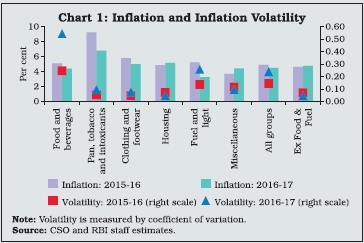 Headline and core inflations may diverge in the wake of relative price shocks. If headline inflation reverts to core inflation, the role of food and fuel price shocks is considered transitory. On the other hand, if core inflation catches up with headline inflation, it suggests a generalised movement in prices through second round effects and inflation expectation channels (Anand, et al. 2015). The observed deceleration in headline inflation in India in the recent period could, therefore, potentially be a transitory phenomenon in the wake of sharp correction in food prices and favourable terms of trade aided by a decline in global commodity prices. Measuring inflation persistence is widely addressed in empirical literature starting with the seminal work of Rotemberg (1982) which relied on nominal price contracting to impart a degree of inertia in a rational expectation setting. Drawing on literature, inflation persistence was tracked by autoregressive behaviour. The autoregressive coefficients, using an ARIMA model on a de-seasonalised CPI from January 2011 to March 2017, corroborated persistence in inflation, both at the overall and sub-group levels, barring housing, and transport and communication (Table 1). However, the degree of persistence varied across sub-groups. For example, the level of inflation persistence was found to be relatively high for services components such as health and education. Moreover, health and education inflation had lower volatility, suggesting relatively steady inflation. The persistence in inflation could be attributable to multitudes of factors such as market structure, levels of productivity and habit formation. Intensifying competition in goods and services markets coupled with productivity enhancing measures could help address persistence in inflation more on a durable basis. During April-June 2017-18, inflation excluding food and fuel declined and persistence also faded across all sub-groups. This is also reflected in the out-of-sample forecast performance of the ARIMA model. Possible pass-through of lower headline inflation in recent months to core inflation could have worked through second-round effects and inflation expectations. | Table 1: Measurement of Persistence: 2011 (January) - 2017 (March) | | | Mean Standard Deviation | Persistence | Inflation
(Y-o-Y) | AR(1) | Sum of AR Coefficients up to 2 lags | | Pan, tobacco and intoxicants | 9.2 | 1.9 | 0.99* | 0.97 | | Clothing | 8.5 | 3.0 | 1.25* | 0.99 | | Footwear | 7.4 | 3.0 | 0.99* | 0.99 | | Housing | 6.6 | 1.8 | -0.15 | -0.14 | | Health | 6.0 | 1.3 | 0.51* | 0.97* | | Education | 7.3 | 1.6 | 0.65* | 0.96* | | Personal care and effects | 6.2 | 3.8 | 1.01* | 0.92 | | Recreation and amusement | 4.9 | 0.9 | 0.67* | 0.84 | | Transport and communication | 3.9 | 3.1 | -0.31 | -0.14 | | Excluding food and fuel | 6.4 | 1.9 | 0.46 | 0.58* | | *: Significant at 5 per cent level. | References: 1. Anand, R., E. Prasad and B. Zhang (2015), “What Measure of Inflation Should a Developing Country Central Bank Target?”, IMF Working Paper, WP/15/205. 2. Laflèche, T. and J. Armour (2006), “Evaluating Measures of Core Inflation”, Bank of Canada Review, pp. 19-29. 3. Rotemberg, Julio J. (1982), “Sticky Prices in the United States’’, Journal of Political Economy, 90(6), December. | II.2.3 On an annual average basis, inflation came down to 4.5 per cent in 2016-17 from 4.9 per cent in the previous year in a fairly generalised movement, except in the housing and miscellaneous categories (Appendix Table 4). Household’s inflation expectations adapted to salient price movements and broadly tracked inflation developments over the year as reflected in the March 2017 round of the Reserve Bank’s inflation expectations survey conducted during the year. An ebbing of inflation expectations was also corroborated in various rounds of the more forward-looking responses in the survey of professional forecasters. II.2.4 Inflation edged up in a number of economies to or above target levels in 2016-17, reflecting tighter labour market conditions and the firming up of commodity prices, especially crude oil and metals. Turkey and South Africa remained outliers in an otherwise low inflation environment (Chart II.11). 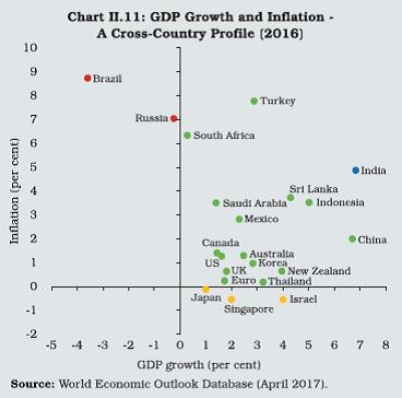 II.2.5 Globally, prices of agricultural commodities, especially food items, firmed up during the year due to a moderation in excess supply (Chart II.12). Metal prices also hardened due to higher real estate investments and efforts for reduction of excess industrial capacity in China, which accounts for more than half of the global consumption of metals. Easing of fiscal policy in the United States also supported the firming up of global metal prices. Global crude oil prices trended up after the OPEC’s November 2016 decision to cut production by around 1.2 million barrels per day, effective January 01, 2017 to bring the ceiling to 32.5 million barrels per day in the first half of 2017. The price of the Indian basket of crude oil moved in tandem and rose to about US$ 51 per barrel in March 2017 from around US$ 36 per barrel in March 2016. Constituents of Inflation II.2.6 Intra-year movements in headline inflation were underpinned by significant shifts at the sub-group level. Broadly, there was a sharp decline in the contribution of food and beverages in H2: 2016-17, while that of non-food components, notably transport and communication, and fuel and light, picked up. Housing and services such as health and education were the other drivers of inflation (Chart II.13). Food II.2.7 Inflation in food and beverages (weight: 45.9 per cent in CPI), declined the most during 2016-17, with its contribution to overall inflation down to 46 per cent from 49 per cent a year ago. Both kharif and rabi seasons produced bumper harvests, aided by a normal monsoon after two consecutive years of drought-like conditions. As stated earlier, distress sales of vegetables and other perishables following demonetisation accentuated the loss of momentum in food prices. In January 2017, food inflation touched an intra-year trough of 1.4 per cent, although prints in May and June took it down even lower to (-) 0.2 per cent and (-) 1.2 per cent, respectively (Chart II.14). 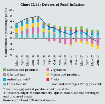 II.2.8 Perishable items - primarily vegetables - that account for 13 per cent of the food group in CPI were the principal agents driving the collapse of food inflation. Vegetable prices faced an unprecedented downturn in August 2016 following significantly higher arrivals in mandis relative to the seasonal pattern. The loss of momentum intensified from Q3 with demonetisation and fresh winter crop arrivals (Chart II.15). II.2.9 While there was a sharp decline in prices of inflation-sensitive vegetables such as potatoes and tomatoes that typically provide the inflexion points in the trajectory of inflation, this time around it was the price of vegetables like cabbages, cauliflowers and peas that plunged disproportionately providing tangential evidence of distress sales and re-deployment of supplies towards urban areas post-demonetisation. CPI-urban food inflation declined faster than its rural counterpart (Chart II.16). II.2.10 The evolution of food prices from August 2016 points towards a possible role of non-transitory factors in bringing down inflation as reflected in a statistically significant break in the series. This was corroborated by the vegetable price series, in particular. II.2.11 Excluding vegetables, average food inflation would have been higher by 2.2 percentage points during August 2016-January 2017 (Chart II.17). II.2.12 Pulses, with a weight of 5 per cent in the food group, contributed substantially to the large swings in food inflation during the year. Their contribution to overall inflation shifted from (+) 12.6 per cent in the first half to (-) 3.6 per cent in the second half of the year. II.2.13 At a granular level, inflation in terms of arhar and urad prices, which drove up inflation in the whole category during 2015-16 and in the beginning of 2016-17, slid down substantially and even deflated in the second half of the year (Chart II.18). Arhar prices at the mandi level in the major producing states of Maharashtra, Madhya Pradesh, Gujarat and Karnataka dropped even below the minimum support price (MSP). Gram was an outlier with an unprecedented surge in prices during 2016-17, barring Q4. After two consecutive years of shortfalls, pulses production increased substantially to 23.0 million tonnes in 2016-17 from 16.4 million tonnes in the previous year in response to a normal rainfall and a significant increase in acreage incentivised by policy interventions, including an increase in MSP. Other supply management measures taken by the government such as imports at zero duty, extension in stockholding limits for traders and building of buffer stocks also helped to rein in pulses inflation. 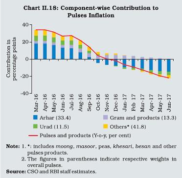 II.2.14 Within the overall moderation, sugar and confectionery posted double-digit inflation, reflecting a drop in sugar production. In response, the government put in place a number of price control measures including imposition of stockholding limits on traders, discouraging exports of sugar and allowing imports of raw sugar. Cereals and prepared meals also showed upside impulses in prices during the year. The dwindling of wheat stocks below the quarterly buffer norm, beginning August 2016, prompted supply-side measures in the form of reduction in import duty to zero in December 2016 that led to an upsurge in imports. Fuel II.2.15 The fuel group (6.8 per cent weight in the CPI) contributed 4.8 per cent to headline inflation during the year, down from 7.1 per cent a year ago. Changes in administered prices of coal, electricity and LPG and hardening of prices of other household fuels including firewood and chips led to fuel inflation increasing from an average of 2.9 per cent till November 2016 to 4.1 per cent thereafter. While in the case of kerosene there was a reduction in subsidy, domestic LPG prices rose in line with international prices. As a result, input cost pressures picked up, especially with respect to raw materials and intermediates. Non-Food, Non-Fuel II.2.16 CPI inflation excluding food and fuel remained sticky through the year with a modest ebbing since April 2017 (Chart II.19). Inflation in transport and communication shot up from 0.7 per cent in May 2016 to 6.0 per cent in March 2017, reflecting the increase in international crude oil prices. Housing inflation increased during the year, although its contribution to inflation excluding food and fuel remained stable. Inflation in personal care and effects remained high till Q3 before declining in the last quarter. II.2.17 Items that showed a moderation in inflation included clothing and footwear, pan, tobacco and intoxicants and services such as household goods and services, health and recreation and amusement. Inflation excluding food, fuel and petrol and diesel components of transportation averaged 4.9 per cent in 2016-17, down from 5.2 per cent in the previous year. Other Indicators of Inflation II.2.18 In April 2017, the Ministry of Commerce and Industry revised the base year for the Wholesale Price Index (WPI) from 2004-05 to 2011-12 in sync with CPI. WPI inflation, based on the new series, ruled higher than CPI inflation from January 2017, reflecting the rise in global commodity prices, particularly crude oil and metals. WPI inflation reached an intra-year peak of 5.5 per cent in February 2017 before easing under the influence of fuel and power group. As such, the narrowing of the gap between measures of inflation based on CPI and WPI, which started in October 2015, got reversed in January 2017 before its re-emergence in June 2017. II.2.19 The WPI series is now akin to the Producer Price Index (PPI) as the former excludes indirect taxes. The coverage of WPI was raised to 697 items from 676 and the number of quotations to 8,331 from 5,482. The primary articles’ group is now weighted higher while the weights of fuel and power and manufactured products have decreased. In consonance with CPI and international practices, item level aggregation for WPI is based on geometric mean as against arithmetic mean in the old series. The number of 2-digit groups in manufactured products has been increased from 12 to 22 as per the National Industrial Classification (NIC) - 2008. The index for electricity is now compiled as a unified item as against the earlier practice of separate sectoral indices such as for agriculture and industry. A high level standing Technical Review Committee, headed by Secretary, Industrial Policy and Promotion has been set up to review and dynamically update the item basket in tune with the changing structure of the economy. II.2.20 WPI inflation as per new series was lower during 2016-17 than that based on the old series, even as trends in inflation - overall and major sub-group- wise - remained largely unchanged in the new series (Chart II.20). II.2.21 For the year as a whole, while inflation as measured by WPI and GDP/GVA deflators increased during 2016-17, sectoral CPI inflation based on CPI-IW, CPI-AL and CPI-RL eased in line with the overall CPI inflation. Following the rise in global crude oil and metal prices, domestic farm and non-farm input costs posted considerable escalation in the second half of 2016-17. Moderate increases in MSPs were announced during the year for crops such as cereals and coarse grains, while the government continued to incentivise the production of pulses and oilseeds by raising their MSPs along with a hike in bonus for pulses. II.2.22 Rural wage growth firmed up from August 2016, both for agricultural and non-agricultural labourers. In the corporate sector, staff costs as a proportion of the value of production moved up during the year even as pricing power gradually returned with improvements in demand conditions. II.2.23 In sum, during 2016-17 CPI inflation ebbed significantly largely reflecting the sharp downturn in the prices of pulses and vegetables following bumper production and supply management measures and later accentuated by the transitory effects of demonetisation. Nonetheless, upside risks may emerge from input costs, wages and imported inflation. II.3 MONEY AND CREDIT II.3.1 Several significant developments fundamentally impacted the evolution of monetary aggregates during 2016-17. Up to October 2016, market operations, intended to balance system-level liquidity, set the path of reserve money and money supply. Thereafter, demonetisation and its after-effects, i.e., initial limits on cash withdrawals, war-time operations to absorb the resultant liquidity overhang and the rapid pace of remonetisation, altered their paths drastically as portrayed in sub-sections 1 and 2. Somewhat obscured underneath these tectonic shifts, was a large redemption of FCNR(B) deposits swapped with the Reserve Bank at the time of the taper tantrum, with counter-balancing operations to even out the liquidity effects. During the year, a combination of factors also restrained the demand for and supply of bank credit (as brought out in sub-section 3) and consequently, the mobilisation of deposits. Box II.5 revisits the relationship between credit and output in the context of the seismic changes in monetary conditions during the year. Since January 2017, however, the monetary aggregates are progressively realigning with their usual patterns. 1. Reserve Money II.3.2 Over the first seven months of 2016-17, the behaviour of reserve money (RM) was largely conditioned by the stance of liquidity management– the Reserve Bank’s resolve in its April 2016 bi-monthly policy statement of progressively moving ex ante liquidity in the system towards neutrality. In terms of components, currency in circulation (CIC) rose sharply in Q1 but fell back in Q2, reflecting the usual seasonality. Buoyed by festival demand and a bumper kharif harvest, a renewed pick-up in CIC was beginning to form in Q3 when demonetisation abruptly stifled it. On November 4, 2016, CIC had scaled an all-time high of ₹18 trillion taking RM to a peak of ₹22.5 trillion. During this seven-month period, bankers’ balances with the Reserve Bank – the other component of RM – unwound from the usual balance sheet related build up at the end of March 2016 and banks generally economised on their holdings of excess reserves in view of the Reserve Bank’s liquidity provision operations in consonance with its stance including the reduction in daily maintenance requirements with respect to the cash reserve ratio (CRR) from 95 per cent to 90 per cent. II.3.3 Demonetisation imposed a compression on the level and path of RM. Following the withdrawal of legal tender status of specified bank notes (SBNs) on November 9, 2016, CIC fell precipitously to a low of ₹9 trillion on January 6, 2017 (around 50 per cent of the peak), a level seen more than six years ago. While banks’ vault cash shot up in the immediate aftermath, it quickly dropped as the Reserve Bank mounted unprecedented liquidity absorption operations (see Chapter III) to mop up the massive influx of liquidity as SBNs were returned by the public. As a result of these large changes, a downward spiral in RM took it down to ₹13.8 trillion (61 per cent of the peak) by January 6, 2017. II.3.4 As remonetisation gathered pace, CIC moved up week after week and reached 74.3 per cent of the peak by the end of the financial year. At end-March 2017, CIC amounted to 8.8 per cent of GDP, down from 12.2 per cent in the previous year. At this level, India’s currency to GDP ratio compares well with a host of advanced and emerging market economies (such as Germany, France, Italy, Thailand and Malaysia). II.3.5 As in the past, scheduled commercial banks (SCBs) built up sizable year-end balances, even as excess reserves maintained by them came down to 17 per cent at end-March 2017 from 23 per cent a year ago (Chart II.21). This reflected the abundance of liquidity following demonetisation. II.3.6 For the year as a whole, RM contracted by around 13 per cent for the first time after 1952-53, as against a similar order of expansion in 2015-16. CIC declined by ₹3.3 trillion, while bankers’ balances with the Reserve Bank increased by ₹423 billion. As at end-March 2017, the net Reserve Bank credit to banks and commercial sector declined by ₹6.1 trillion vis-à-vis an increase of ₹1 trillion in the previous year. II.3.7 On the sources side, the year began with considerable turbulence in global financial markets amidst worries about global growth. With capital influx dwindling, accretions to net foreign assets (NFAs) through net purchases from authorised dealers (ADs) were relatively muted during Q1 (Chart II.22). Compensating variations in net domestic assets (NDAs) to ensure a neutral liquidity position took the form of net open market operations (OMOs), i.e., purchases of ₹805 billion in Q1 of 2016-17 as against net OMO sales of ₹51 billion in Q1 a year ago. As financial markets priced in the Brexit referendum, capital inflows resumed in Q2 and accordingly, the pace of OMO purchases moderated to ₹200 billion. Net purchases from ADs increased from ₹78 billion in Q1 to ₹680 billion in Q2. Furthermore, the transfer of the Reserve Bank’s surplus of ₹659 billion in August 2016 augmented spending by the government and added to the liquidity in the banking system. 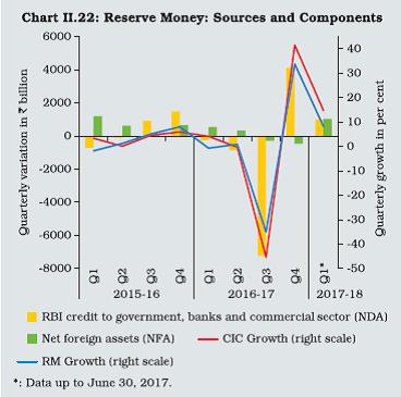 II.3.8 During the third quarter of the fiscal year, the sources of RM underwent significant changes after demonetisation unleashed a wave of liquidity into the system. Initially, reverse repos under the liquidity adjustment facility (LAF) were the principal instrument of absorption, bringing net Reserve Bank credit to banks and the commercial sector down to ₹(–)5.2 trillion as on November 25, 2016 from ₹3 trillion at the beginning of the year. As surplus liquidity mounted, the Reserve Bank imposed an incremental CRR of 100 per cent of the increase in net demand and time liabilities (NDTL) (between September 16, 2016 and November 11, 2016) on November 26, 2016. This temporary impounding of liquidity of the order of about ₹4 trillion was withdrawn from December 10, 2016 with the enhancement of the ceiling on issuance under the market stabilisation scheme (MSS) to ₹6 trillion from ₹300 billion. As the MSS issuances grew and liquidity was sequestered, net Reserve Bank credit to the government declined from ₹4.2 trillion at the beginning of the year to a low of ₹37 billion by December 23, 2016. The outstanding MSS issuances peaked at ₹6 trillion as on January 6, 2017. While remonetisation gathered pace, MSS issuances matured by mid-March, and LAF reverse repo re-emerged as the principal instrument of liquidity absorption. The government’s cash balances also declined by ₹613 billion by end- March 2017 and as a result, net Reserve Bank credit to the government increased to ₹6.2 trillion by the end of the year vis-à-vis ₹4.2 trillion a year ago. II.3.9 A comparison of the Reserve Bank’s balance sheet size pre- and post-demonetisation shows a decline of ₹0.8 trillion (2.4 per cent) during November 4, 2016 through March 31, 2017 as against an increase of ₹4.7 trillion (16.1 per cent) in the corresponding period a year ago. Moreover, the composition of liabilities changed significantly, with the share of the largest component, viz., notes in circulation declining sharply from 54.3 per cent as on November 4, 2016 to 27 per cent as on January 6, 2017 before increasing to 41.1 per cent at end-March 2017. Furthermore, the MSS impound and other deposits (mainly LAF reverse repo with banks) increased significantly. The switch from non-interest bearing currency liabilities to interest bearing deposits, coupled with a decline in the Reserve Bank’s credit to banks, has implications for the Reserve Bank’s surplus. II.3.10 In 2017-18 (upto June 30), with CIC falling short of its level a year ago by ₹2.0 trillion, RM was lower by 5.6 per cent. CIC, in fact, was placed at 85.2 per cent of its pre-demonetisation level on June 30, 2017. Bankers’ deposits increased by 16.2 per cent as compared to 13.1 per cent in the corresponding period of the previous year, reflecting a surge in deposits in the banking system. Net Reserve Bank credit to the government and to the banks and the commercial sector drove down the RM, offsetting the upward push from net purchases from authorised dealers. 2. Money Supply II.3.11 The year-on-year growth of money supply (M3) slackened during 2016-17, reflecting subdued credit growth and a sizable redemption of FCNR (B) deposits. Barring a short-lived spike during Diwali, the deceleration became sharper in the second half following demonetisation. II.3.12 Turning to the components of money supply, currency with the public largely followed the patterns of CIC discussed in the preceding section. Aggregate and demand deposits follow a seasonal pattern akin to currency with the public, while time deposits are largely stable. However, in 2016-17, aggregate deposits increased sharply in Q2 on account of the release of the 7th CPC award of salaries and pension arrears and mobilisation of deposits under the income declaration scheme. In terms of year-on-year growth, however, aggregate deposits decelerated till October 28, 2016 largely in line with subdued credit growth. Following demonetisation, deposits accelerated sharply as these substituted the currency with the public (Table II.4). The pace of deposits turned somewhat tempered by the redemption of FCNR(B) deposits mobilised under the Bank’s swap scheme, which coincided with demonetisation. As a result, the increment in deposits post-demonetisation till mid- February was less than the contraction in currency with the public (Chart II.23). The M3 growth in 2017-18 (upto June 23, 2017) at 7.4 per cent remained much lower than the growth registered in the corresponding fortnight last year (10.3 per cent). | Table II.4: Monetary Aggregates | | Item | Outstanding as on March 31, 2017 (₹ billion) | Year-on-year growth (per cent) | | 2015-16 | 2016-17* | 2017-18
(as on June 23) | | 1 | 2 | 3 | 4 | 5 | | I. Reserve Money (RM) | 19,005 | 13.1 | -12.9 | -5.6 | | II. Broad Money (M3) | 128,444 | 10.1 | 7.3 | 7.4 | | III. Major Components of M3 | | | | | | 1. Currency with the public | 12,637 | 15.2 | -20.8 | -12.6 | | 2. Aggregate deposits | 115,596 | 9.4 | 11.6 | 10.6 | | IV. Major Sources of M3 | | | | | | 1. Net bank credit to government | 38,691 | 7.7 | 21.0 | 14.1 | | 2. Bank credit to commercial sector | 84,514 | 10.7 | 4.7 | 5.7 | | 3. Net foreign exchange assets of the banking sector | 25,582 | 12.6 | 1.1 | 1.5 | | V. M3 net of FCNR(B) | 127,084 | 10.1 | 8.9 | 9.1 | | M3 Multiplier | 6.8 | | | | Note : The data for RM pertain to June 30, 2017.
* : March 31, 2017 over April 1, 2016 barring for RM. |
 II.3.13 On the sources side, the growth in net bank credit to the government accelerated sharply reflecting the quantum increase in banks’ investment in government securities in the context of a surge in deposits following demonetisation. On the other hand, growth in credit to the commercial sector moderated during the year mainly due to lower credit growth of PSBs. II.3.14 The extraordinary developments during the year – exchange of notes/deposits – had a fundamental impact on the money multiplier. In contrast to the previous year, the currency-deposit (c/d) ratio underwent a steep fall due to the contraction in currency with the public and the concomitant increase in deposits. On the other hand, the reserve-deposit (r/d) ratio remained largely stable, barring the fortnight when the incremental CRR of 100 per cent was applied and the last fortnight of the financial year. The money multiplier, which hovered around 5.5 in the pre-demonetisation phase, scaled up to peak at 8.8 by early January 2017. As remonetisation quickened, the money multiplier declined gradually but remained elevated relative to its own history at 6.8 at end-March 2017 (5.3 a year ago). Adjusted for reverse repo (net) with banks – analytically akin to banks’ deposits with the central bank – the money multiplier, however, turned out to be lower and aligned to its pre-demonetisation level at 5.8 at end-March 2017 vis-à-vis 6.2 a year ago (Chart II.24).  3. Credit II.3.15 The growth in non-food credit extended by scheduled commercial banks (SCBs) reached a low of 5.8 per cent at end-March 2017, the lowest since 1994-95 (10.9 per cent in the previous year). Banks typically build up credit portfolios at the end of the year for balance sheet considerations. Non-food credit expansion in the last fortnight accounted for 74.2 per cent of the annual increase (38.3 per cent in the previous year). Excluding this window-dressing, non-food credit growth as on March 17, 2017 was even lower at 5.1 per cent vis-à-vis 10.9 per cent on the corresponding day in the previous year. A combination of factors drove down credit growth despite softening of lending rates – the subdued state of economic activity (Box II.5); risk aversion in the banking sector with a legacy of NPAs and capital adequacy requirements acting as a binding constraint on banks; and disintermediation via increasing recourse to market-based instruments, such as commercial papers (CPs) and corporate bonds. Credit growth was also impacted by one-off/statistical factors such as loan write-offs, substitution of bank credit by UDAY bonds, loan repayment by use of SBNs and banks’ pre-occupation with exchange of notes/deposits following demonetisation. Even inclusive of CPs, non-food credit growth during 2016-17 was lower at 6.4 per cent as against 10.2 per cent in the previous year. Real credit growth showed a sharp deceleration to 1.8 per cent from 5.8 per cent a year ago. In terms of intra-year variations, non-food credit flow dipped albeit a little more than usual in the first quarter of 2016-17 before posting a sharp recovery in the next quarter – a contrast to its customary behaviour (Chart II.25). While non-food credit flows started receding thereafter, a declining momentum got entrenched in the aftermath of demonetisation. However, it recovered somewhat towards the end of the fourth quarter of 2016-17, reflecting the usual year-end window dressing. During 2017- 18 (upto June 23, 2017), NFC growth remained lower at 6.7 per cent when compared with the growth of 9.3 per cent in the corresponding period of the previous year. 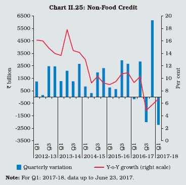
Box II.5
Credit and Output: Macro and Sectoral Dimensions Bank lending accounted for around 50 per cent of the total flow of resources to the commercial sector in 2015-16 and about 37 per cent in 2016-17. In a bank-based economy, bank credit is considered critical in determining output (Korkmaz, 2015). Higher credit growth is expected to lead to higher GVA growth and vice versa. However, in recent years, there appears to be a disconnect in the growth rates of credit and GVA in India (Chart 1). The anaemic growth in bank credit in the recent period is attributed to various factors such as stressed assets, subdued economic activity and sticky capacity utilisation. Nevertheless, the data on sectoral deployment of credit reveal divergence in credit growth across sectors (Chart 2). For example, credit for agriculture and allied activities, and personal loans showed healthy growth, while flows to industry and services sectors were subdued. The quarterly seasonally adjusted data on real bank credit and GVA for 1996-2017 and sectoral credit for 2007-17 were found to be non-stationary in levels but stationary in first difference. Following Izz and Ananzeh (2016), a co-integrating relationship and a significant error correction mechanism were found between GVA and credit (at aggregate and sectoral levels). A long-run co-integrating relation between credit and GVA has been estimated as: Log (gva)=6.99+0.64*log (bc)………..(1) where gva=real GVA; bc=real bank credit. Dummies for 2009-10 Q2 to 2012-13 Q1 (identified through least squares with breakpoints) and for 2015-16 Q2 to 2016-17 Q4 were used to account for the global financial crisis and asset quality review of banks by the Reserve Bank, respectively. Equation (1) indicates that with every 1 per cent increase in real credit, real GVA increases by 0.64 per cent. Further, the error correction term has a negative sign and is statistically significant, implying that the underlying mechanism corrects disequilibrium. The estimated long-run co-integrating relation between GVA and sectoral credit is: Log (gva)=5.26+0.58*log(agr_cr)-0.006*log(ind_cr) + 0.53*log (ser_cr)………..(2) where agr_cr= real credit to agriculture; ind_cr= real credit to industry; and ser_cr= real credit to services sector. Dummy was used for the period since the asset quality review of banks by the Reserve Bank. At a sectoral level, credit to agriculture and services was associated with higher output; however, industrial credit was not found to be statistically significant, possibly reflecting substitution by other sources of finance such as commercial papers and corporate bonds (RBI 2015). The large and statistically significant coefficient of services’ credit may be seen in the context of an increase in the share of the services sector’s credit in total non-food credit from 23 per cent in 2007 to 26 per cent in 2017. The healthy growth in credit to the services sector in recent years was driven by professional services, retail trade, NBFCs and transport operators. To sum up, while the relationship between credit and GVA still holds at the aggregate level, increasing substitution of industrial credit by alternative sources against the backdrop of impaired assets in banks seems to have weakened the relation between industrial credit and output. References: Izz Eddien and N. Ananzeh (2016), ‘‘Relationship between Bank Credit and Economic Growth: Evidence from Jordan’’, International Journal of Financial Research, 7(2). Korkmaz, Suna (2015), ‘‘Impact of Bank Credits on Economic Growth and Inflation’’, Journal of Applied Finance & Banking, 5(1). Reserve Bank of India (2015), ‘‘Box II.4: Factors Underlying Recent Credit Slowdown: An Empirical Exploration’’, Annual Report 2014-15, page No. 32. | II.3.16 Among bank groups, public sector banks trailed behind private banks in terms of credit growth during 2016-17, a secular-like movement evident since 2011-12. Credit to all major sectors, barring services, decelerated/contracted during 2016-17 (Table II.5). Credit to agriculture slowed down to 12.4 per cent from 15.3 per cent in the previous year. | Table II.5: Sectoral Credit Deployment by Banks | | Sectors | Outstanding as on March 31, 2017 (₹ billion) | Year-on-year growth (per cent) | | 2015-16* | 2016-17# | 2017-18$ | | 1 | 2 | 3 | 4 | 5 | | Non-food Credit (1 to 4) | 7,0947 | 9.1 | 8.4 | 4.8 | | 1 Agriculture & allied activities | 9,924 | 15.3 | 12.4 | 7.5 | | 2 Industry (micro & small, medium and large) | 26,800 | 2.7 | -1.9 | -1.1 | | (i) Infrastructure | 9,064 | 4.4 | -6.1 | -2.5 | | Of which: | | | | | | (a) Power | 5,254 | 4.0 | -9.4 | -1.6 | | (b) Telecommunications | 851 | -0.7 | -6.8 | -9.1 | | (c) Roads | 1,800 | 5.2 | 1.4 | -6.5 | | (ii) Basic metal & metal product | 4,211 | 7.9 | 1.2 | -1.0 | | (iii) Food processing | 1,455 | -12.5 | -3.1 | -0.7 | | 3 Services | 18,022 | 9.1 | 16.9 | 4.7 | | 4 Personal loans | 16,200 | 19.4 | 16.4 | 14.1 | | Priority sector | 24,357 | 10.7 | 9.4 | 4.0 | Note : Data are provisional and relate to select banks which cover about 95 per cent of the total non-food credit extended by all SCBs.
* : March 18, 2016 over March 20, 2015; #: March 31, 2017 over March 18, 2016.
$ : June 23, 2017 over June 24, 2016. | II.3.17 Credit to industry, particularly infrastructure, food processing and iron and steel segments, has been contracting since October 2016. Credit to industry contracted by 1.9 per cent during 2016-17 in contrast to a growth of 2.7 per cent in the previous year. Credit to infrastructure (which accounts for about one-third of the outstanding bank credit to industry) contracted by 6.1 per cent in 2016- 17 on top of a low growth of 4.4 per cent in the previous year. Within infrastructure, credit growth contracted/decelerated in respect of all major segments such as power, telecommunication and roads. Credit to textiles and engineering goods also slowed. However, credit to fertilisers, petro chemicals and construction activity accelerated sharply. II.3.18 The overall contraction in credit to industry was due to the inter-play of several factors. First, investment activity has been weak in recent years, which has severely impacted credit offtake. Second, within industry, several sector-specific factors contributed to contraction in credit. For example, the power sector, which accounts for about 58 per cent of the outstanding credit to infrastructure, has been facing hurdles like stalled projects, operational inefficiencies and high outstanding debt. Telecommunication industries were experiencing declining revenue and a grim profit outlook due to technological innovations and stiff competition among the service providers. The iron and steel sector was stressed due to weak prices and stiff international competition. II.3.19 Belying the general trend, personal loans continued to grow at a healthy rate, although the growth was somewhat lower (16.4 per cent vis-à- vis 19.4 per cent in the previous year) due to marked deceleration in housing loans which constituted more than half of the outstanding credit to this sector. Credit to consumer durables and vehicles also grew at a healthy rate. Credit flow to the services sector improved significantly to 16.9 per cent from 9.1 per cent last year led by the professional services and trade. II.3.20 During 2017-18 (up to June 2017), overall credit slowdown has persisted with most sectors witnessing deceleration or contraction. While credit to industry continued to contract, credit growth to agriculture slowed down significantly to 7.5 per cent in June 2017 from 13.8 per cent in the corresponding period of the previous year. Credit to the services sector decelerated sharply, reflecting slowdown across all its sub-components, barring trade and other services. II.3.21 During 2016-17, the flow of financial resources to the commercial sector declined, largely mirroring the anaemic non-food credit (Table II.6). In contrast, banks’ non-SLR investment increased sharply by 47.2 per cent while the flow of resources from non-banks recorded an uptick. Within non-bank sources, notably, private placements by non-financial entities and CPs subscribed by non-banks increased during the year. Among foreign sources, external commercial borrowings (ECB)/foreign currency convertible bonds (FCCB) recorded net outflows for the second year in a row, while the flow of FDI was largely sustained. | Table II.6: Flow of Financial Resources to Commercial Sector | | (₹ billion) | | | 2014-15 | 2015-16 | 2016-17 | 2016-17
Apr-June | 2017-18
Apr-June | | 1 | 2 | 3 | 4 | 5 | 6 | | A. Adjusted non-food bank credit | 5,850 | 7,754 | 5,025 | 263 | -1,927 | | i) Non-Food credit | 5,464 | 7,024 | 3,950 | -168 | -1,886# | | of which: petroleum and fertiliser credit | -139 | -18 | 134 | -23 | -133 | | ii) Non-SLR investment by SCBs | 386 | 731 | 1,075 | 431 | -41# | | B. Flow from Non-banks (B1+B2) | 7,005 | 7,358 | 9,257 | 1,276 | 1,654 | | B1. Domestic sources | 4,740 | 4,899 | 6,499 | 1,185 | 1,166 | | 1 Public issues by non-financial entities | 87 | 378 | 155 | 29 | 52 | | 2 Gross private placements by non-financial entities | 1,277 | 1,135 | 2,004 | 240 | 240 | | 3 Net issuance of CPs subscribed to by non-banks | 558 | 517 | 1,002 | 720 | 148 | | 4 Net credit by housing finance companies | 954 | 1,188 | 1,346 | 110 | 225* | | 5 Total accommodation by 4 RBI regulated AIFIs - NABARD, NHB, SIDBI & EXIM Bank | 417 | 472 | 469 | 15 | 108 | | 6 Systemically important non-deposit taking NBFCs (net of bank credit) | 1,046 | 840 | 1,245 | 35 | 285 | | 7 LIC’s net investment in corporate debt, infrastructure and social sector | 401 | 369 | 277 | 36 | 108 | | B2. Foreign Sources | 2,265 | 2,459 | 2,758 | 91 | 488 | | 1 External commercial borrowings/FCCB | 14 | -388 | -509 | -167 | 11 | | 2 ADR/GDR Issues excluding banks and financial institutions | 96 | 0 | 0 | 0 | 0 | | 3 Short-term credit from abroad | -4 | -96 | 435 | -23 | - | | 4 Foreign direct investment to India | 2,159 | 2,943 | 2,833 | 281 | 477* | | C. Total Flow of Resources (A+B) | 12,855 | 15,112 | 14,282 | 1,539 | -273 | | Memo: Net resource mobilisation by Mutual Funds through debt (non-gilt) Schemes | 49 | 147 | 1,206 | 388 | 191 | Note: *: Up to May 2017; #: Up to June 23, 2017.
Source: RBI, SEBI, BSE, NSE, Merchant Banks, LIC, NHB and NSDL. | II.3.22 The primary issuance of corporate bonds was dominated by private placements vis-à-vis public issues, with the former constituting 95.7 per cent of total issuance in 2016-17, up from 92.1 per cent in the previous year. Further, the share of financial entities as against non-financial entities in the resource mobilisation through corporate bonds increased to 71.7 per cent from 71.2 per cent over the same period. During 2017-18 (up to June 2017), the share of financial entities increased further to 84.6 per cent over the previous year. II.3.23 In sum, the evolution of monetary and liquidity conditions during 2016-17 were shaped by developments such as the withdrawal of SBNs, redemption of FCNR (B) deposits, liquidity management stance of the Reserve Bank and global factors. The fast pace of currency expansion was reversed by demonetisation leading to a surge in liquidity in the system and a slew of measures by the Reserve Bank to manage it. Subdued credit growth and redemption of FCNR(B) moderated money supply growth. With liquidity and currency levels progressing towards neutral/normal, the resolution of stressed assets and recapitalisation of public sector banks will be critical for improving credit off-take. II.4 FINANCIAL MARKETS II.4.1 Sporadic episodes of volatility buffeted global financial markets during 2016-17, largely reflecting uncertainties surrounding the materialisation of political risks such as the unexpected outcome of the Brexit referendum and the results of the US Presidential election. Market sentiment was also unsettled by increased prospects of monetary policy tightening by the US. While markets in advanced economies (AEs) generally relied on reflation trade on perceptions of better growth prospects, those in emerging market economies (EMEs) plunged on fears of capital outflows and the Fed rate hike. Subsequently, however, equity prices recovered in most EMEs as capital outflows ceased and inflows resumed as reflation exuberance subsided and the stance of the US Federal Reserve was read as being less hawkish. II.4.2 In India, financial markets were not immune to global developments, especially in equity and foreign exchange segments but others were mostly driven by domestic factors. In the money market, interest rates remained anchored to the policy repo rate on the strength of changes in the Reserve Bank’s liquidity management framework in April 2016. In the government securities (G-sec) market, yields generally softened in response to surplus liquidity conditions that were accentuated by demonetisation from November 2016. Abstracting from global spillovers, the equity market surged during the year, largely in response to domestic reforms and improved macroeconomic conditions, as depicted in Box II.6 which evaluates the bull run in the equity market and its sustainability. The domestic forex market remained stable for most part of the year with the Indian rupee (INR) mostly trading with an appreciating bias, except during episodic turbulence caused by global factors. Money Market II.4.3 The money market moved in close sympathy with the stance of the Reserve Bank’s liquidity management framework in April 2016 engendered, inter alia, by (i) smoothening of the supply of durable liquidity; and (ii) progressive lowering of the average ex ante liquidity deficit in the system to a position closer to neutrality. The width of the liquidity adjustment facility (LAF) interest rate corridor between the reverse repo rate and the marginal standing facility (MSF) rate was also lowered from 200 bps to 100 bps in April 2016 with the objective of better aligning the weighted average call rate (WACR) with the policy rate. Further, the minimum daily maintenance of the cash reserve ratio (CRR) was reduced from 95 per cent of the requirement to 90 per cent, effective April 16, 2016. With the introduction of the new liquidity management framework, the Reserve Bank started conducting open market operations (OMO) outright purchases. As a result, the average monthly liquidity deficit in the system consistently declined from April through June 2016. Consequently, WACR remained anchored to the policy repo rate and traded with an easing bias within the policy interest rate corridor. Other money market rates evolved in close alignment with WACR (Chart II.26). 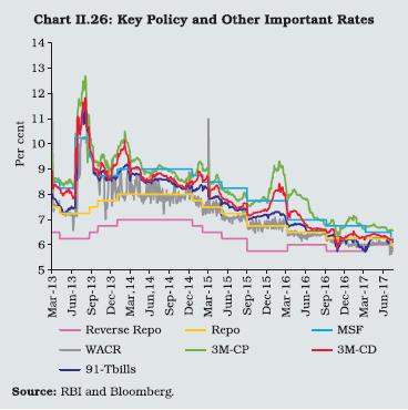 II.4.4 During Q2, overnight money market rates continued to soften and, on an average, remained 10 bps below the policy rate, reflecting the surplus liquidity conditions emanating from a decline in government cash balances and injection of durable liquidity through OMO outright purchases. The rates moderated further following the 25 bps reduction in the policy repo rate in early October. II.4.5 Demonetisation in November led to a significant softening of money market rates lasting till the end of the financial year. Notwithstanding the unprecedented surplus liquidity conditions, money market rates were generally aligned with the policy rate with a downward bias from December 2016, mainly on account of proactive liquidity management by the Reserve Bank involving, inter alia, temporary imposition of the incremental CRR (ICRR) during the fortnight beginning November 26, 2016, issuance of securities under the market stabilisation scheme (MSS) and absorption through the overnight fixed rate reverse repo and variable rate reverse repos of various tenors ranging from overnight to 91-days. The outstanding issuances under MSS peaked at ₹5,966 billion in mid-January 2017. Alongside, the average daily outstanding net liquidity absorption under LAF increased to ₹2,888 billion during November 09, 2016 to March 31, 2017 from ₹70 billion during November 01-08, 2016. Moreover, the usual financial year-end spike in money market rates remained muted in 2016-17 on account of persistence of surplus liquidity in the system. II.4.6 Average daily volume in the money market [call money, collateralised borrowing and lending obligation (CBLO) and market repo] increased significantly by 32 per cent to ₹1,441 billion during 2016-17 from ₹1,090 billion in 2015-16. Volume in call money, CBLO and market repo segments increased by 13 per cent, 32 per cent and 41 per cent, respectively, during the year. Call money, CBLO and market repo segments accounted for 11 per cent, 59 per cent and 30 per cent, respectively, of the total volume during 2016-17 compared to 12 per cent, 59 per cent and 29 per cent in 2015- 16. During Q1 of 2017-18, average daily volume in money market (call money, CBLO and market repo) increased further to ₹1,575 billion. II.4.7 Surfeit of liquidity with banks and enervated credit growth obviated the need for mobilising bulk deposits and, as a consequence, the issuance of certificates of deposit (CDs) declined substantially. The weighted average effective interest rate (WAEIR) on CDs also declined by 1.8 percentage points in 2016-17. The average fortnightly issuance during Q1 of 2017-18 was lower than Q4 of 2016-17 and there was a marginal uptick in WAEIR during the period. In contrast, issuance of commercial paper (CP) increased by around 28 per cent during 2016-17, partly reflecting the substitution of short-term bank credit with market-based funding by highly rated corporates taking advantage of the lower rates. Weighted average discount rate (WADR) on CPs generally declined during the year. II.4.8 The persistence of easy liquidity conditions resulted in money market rates remaining below the policy rate by an average of 25 bps in April- June 2017. In order to ensure a finer alignment of the operating target with the policy rate, the Reserve Bank narrowed the policy rate corridor to 50 bps from 100 bps in its first bi-monthly monetary policy statement for 2017-18 issued in April. Furthermore, the Reserve Bank undertook issuance of treasury bills (T-Bills) under MSS and OMO sale auctions in addition to regular LAF operations. The average daily outstanding net liquidity absorption under LAF was ₹3,558 billion in Q1 of 2017-18. G-sec Market II.4.9 The aggregate volume of transactions in central and state governments dated securities and T-bills (outright as well as repo) increased by 56 per cent, even as yields generally softened during the year, barring some occasional upticks in Q4 (Chart II.27). II.4.10 In Q1, yields remained range-bound with a softening bias on the back of positive sentiment following a reduction in the policy repo rate on April 05, 2016, the change in the liquidity management stance and reduction in the minimum daily CRR maintenance requirements, coupled with stability in the domestic foreign exchange market, expectations of monetary easing by major central banks and an increased likelihood of a dovish stance of the US monetary policy. Yields, however, hardened transiently in the run up to the Brexit referendum on June 23. II.4.11 Yields continued to soften in Q2 of 2016- 17, tracking positive market sentiments generated by the passage of the constitutional amendment bill enabling the introduction of Goods and Services Tax (GST), coupled with comfortable liquidity conditions. The accommodative policy stance of the monetary policy in early August 2016 also helped to bring down yields, which was sustained through September and early October 2016 when the policy repo rate was reduced by 25 bps. II.4.12 G-sec yields hardened marginally after the release of Federal Open Market Committee (FOMC) minutes in mid-October 2016, which markets read as signalling an imminent raising of rates in the US. The unprecedented surplus liquidity conditions following demonetisation in November 2016 led to a sharp decline in yields, with the 10-year benchmark touching a low of 6.26 per cent on November 24, 2016. Subsequently, yields hardened on announcement of the ICRR, a hike in the MSS ceiling and maintaining of status quo on the policy rate in early December 2016. Yields continued to trade in a narrow range till mid- December 2016. The hike in the Fed fund rate by 25 bps on December 14, 2016 and the perceived rising probabilities of three more such increases in 2017, pushed up yields thereafter. II.4.13 With the policy repo rate held unchanged, a change in the policy stance from accommodative to neutral in February 2017 caused a sharp sell-off in gilts. It was only when positive market sentiments returned post-state election results and the less hawkish stance of the US Fed around mid-March 2017 that a mild softening of yields ensued which lasted till the end of the financial year. II.4.14 Yields hardened moderately in April 2017 following the enunciation of upside risks to Inflation in the minutes of the Reserve Bank’s Monetary Policy Committee meeting, released on April 20, 2017. During May 2017, yields hardened initially tracking the US yields ahead of the outcome of the FOMC meeting on May 03, 2017. Subsequently, yields softened on account of a fall in crude oil prices, issuance of a new 10- year benchmark security and lower than expected Inflation numbers for April 2017. Yields softened further after the monetary policy statement on June 07, 2017 and this trend continued with the yield moving in a range-bound manner following the release of lower reading on CPI Inflation in June 2017. Corporate Debt Market II.4.15 Taking advantage of low yields, the resources mobilised through the corporate bond market increased to ₹6,700 billion during 2016-17 from ₹4,922 billion in the previous year. Corporate bond yields softened during 2016-17, tracking movements in G-sec yields and measures taken by the Reserve Bank and the Government to deepen the corporate bond market. These measures include a hike in the aggregate limit of partial credit enhancement provided by banks, permission to brokers in corporate bond repos, and authorisation of a platform for repo in corporate bonds. The 5-year AAA rated corporate bond yield softened by 0.8 percentage point during the year. However, the yield spread of the 5-year AAA rated corporate bond over 5 year G-sec increased during the year reflecting higher perception of credit risk (Chart II.28). The turnover in the corporate bond market increased by around 44 per cent during 2016-17. Foreign portfolio investment in corporate bonds increased to ₹1.9 trillion at end-March 2017 from ₹1.7 trillion in the previous year and accounted for 76 per cent of the limit as compared to 69 per cent a year ago. 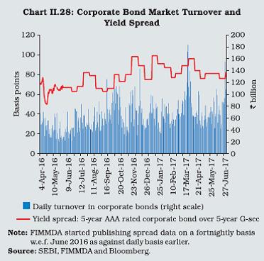 II.4.16 During Q1 of 2017-18, resources mobilised through corporate bonds increased to ₹1,747 billion from ₹1,364 billion in the corresponding period of the previous year. The turnover in corporate bonds also increased substantially to ₹4,347 billion from ₹2,610 billion over the same period. The yield of 5-year AAA rated corporate bonds softened by 16 bps in Q1 of 2017-18. Also, the yield spread of the 5-year AAA rated corporate bond over 5-year G-sec declined by 14 bps reflecting moderation in the perceived credit risk. Equity Market II.4.17 During 2016-17, the benchmark Indian equity indices, i.e., the BSE Sensex and Nifty 50 increased by 16.9 per cent and 18.5 per cent, respectively, remaining generally resilient to multiple shocks during the year (Chart II.29). II.4.18 The stock market surged in the first half of 2016-17 on the back of positive sentiments flowing from the government’s resolve to adhere to fiscal discipline in Union Budget 2016-17, the announcement of structural reform measures (such as, the insolvency and bankruptcy code, and liberalisation of the FDI regime), a normal south-west monsoon, implementation of the 7th Central Pay Commission’s (CPC’s) recommendations and net purchases by foreign portfolio investors amidst favourable cues from global equity markets. II.4.19 Following demonetisation, however, the BSE indices of cash-sensitive sectors such as realty, fast-moving consumer goods (FMCGs) and automobiles declined sharply, indicating market expectations of a fall in demand. The stock markets, however, rallied thereafter on better-than-expected Q3 earnings of companies, optimism over Union Budget 2017-18 proposals to stimulate growth while adhering to the path of gradual fiscal consolidation, revival of foreign portfolio investments with a record net buying in March 2017, better than expected Q3 GDP growth data, passage of the GST Bill in the Lok Sabha and expectations of steady progress on economic reforms. In fact, the BSE Sensex and sectoral indices, except BSE auto, surpassed their pre-demonetisation levels in Q4 of 2016-17, indicating that the impact of demonetisation was only transitory. II.4.20 In Q1 of 2017-18, the BSE Sensex and NSE Nifty 50 increased by 4.4 per cent and 3.8 per cent, respectively in the backdrop of favourable progress in monsoon, perseverance with economic reforms, strong macroeconomic fundamentals and positive cues from global markets. However, the exuberance in the stock markets thus far, has also raised apprehensions about its durability in some quarters (Box II.6). Box II.6
Indian Equity Prices: A Sustainability Analysis The Indian stock markets surged in 2017 vis-à-vis their peers, with the BSE Sensex and NSE Nifty 50 trading at all-time highs with stretched valuations. This has sparked a lively debate as to whether the stock market exuberance is durable (Chart 1). The market price of an asset consists of a fundamental component, i.e., the expected discounted flow of the asset price and a bubble component, which is defined as a dramatic rise in asset prices driven by speculative behaviour, far exceeding its fundamental value. The fundamental component is expected to change fairly gradually over time, while the bubble component can increase in an explosive or exponential manner. The empirical identification of asset price bubbles has been animatedly debated (see, Diba and Grossman 1988). Recognising the limitations of the existing methodologies to identify multiple bubbles in a data series, Phillips, et al. (2015) used a variant of the standard ADF unit root test, viz., the generalised supremum ADF (GSADF) test on the following reduced form equation: where y is the stock price, μ is the intercept, p is the maximum number of lags; θi for i = 1, ..., p are the differenced lags coefficients and ε is the error term. Testing for bubble (explosive behaviour) is based on a right-tail variation of the standard ADF unit root test where the null hypothesis is of a unit root and the alternative is of a mildly explosive autoregressive coefficient, i.e., it tests for H0: δ = 1 and H1: δ > 1. The presence of explosive behaviour in the asset price, i.e., δ > 1 can be taken as evidence of a bubble. This methodology was applied to the Inflation adjusted price-to-dividend ratio of the average monthly BSE Sensex during April 1994 to April 2017, taking the ratio of April 1994 as the baseline. The GSADF test statistic was greater than the critical value at 1 per cent level, possibly indicating evidence of bubbles in the market (Table 1). | Table 1: The GSADF Test for the Sensex 30 Index | | | Test Stat
(p-value) | Finite Sample Critical Values | | 90% | 95% | 99% | | GSADF test | 5.258
(0.000) | 1.92 | 2.14 | 2.93 | Note: Critical values of the GSADF test are obtained from the Monte Carlo simulation with 1000 replications (Caspi 2014). The smallest window has 33 observations.
Source: RBI and BSE. | Chart 2 identifies three major asset price bubble periods during April 1994 to April 2017. The first two bubble periods (June 2005 to May 2006, and August 2006 to February 2008), coincided with the booming phase of FPI inflows and bust after the global financial crisis in 2007-08. Another bubble is identified during August 2014 to February 2015 in the aftermath of the general election results, which ended on concerns over retrospective taxes on FPIs, high valuations and weak earnings growth. No bubble is detected currently when stock prices have reached historical highs. The current rally in stock prices seems to reflect the strong macro fundamentals of the Indian economy, easy liquidity conditions prevailing in the system and buoyancy in global markets. Nonetheless, a constant vigil of stock prices may be warranted at this juncture, keeping in view the ramifications for financial and price stability. References: Caspi, I. (2014), “Rtadf: Testing for Bubbles with EViews”, MPRA Paper No. 58791. Diba, B.T, and H.I. Grossman (1988), “Explosive Rational Bubbles in Stock Prices?” American Economic Review, 78: 520-530. Phillips, P.C.B., S. Shi and J.Yu (2015), “Testing for Multiple Bubbles: Historical Episodes of Exuberance and Collapse in the S&P 500”, International Economic Review, 56(4). | Primary Market Resource Mobilisation II.4.21 The primary segment of the equity market sustained its upward momentum during 2016-17 against the backdrop of improved macroeconomic conditions and policy reforms such as passage of GST Bill. Resource mobilisation through initial public offerings (IPOs) more than doubled to ₹291 billion in 2016-17. The gains in IPO activity were marked by a few mega issues. IPO activity remained subdued during October 2016 to February 2017 in view of the volatility in the stock markets and the post-demonetisation uncertainty, but recovered in March 2017. IPO activity accelerated further during Q1 of 2017-18 as reflected in resource mobilisation of ₹78.6 billion compared to ₹58.6 billion in the same period of the previous year. II.4.22 Resource mobilisation through mutual funds (MFs) more than doubled to ₹3,431 billion in 2016-17 on account of higher mobilisation under income and debt schemes. During Q1 of 2017-18, mutual fund resource mobilisation increased by 3.3 per cent to ₹934 billion from ₹904 billion in the same period of the previous year. Private placement of corporate bonds showed a marked improvement of 39.9 per cent in 2016- 17 vis-à-vis 13 per cent in 2015-16. During Q1 of 2017-18, private placement of corporate bonds increased by 28.3 per cent to ₹1,725 billion from ₹1,345 billion in the corresponding period of 2016- 17. Public issues of non-convertible debentures (NCDs), however, decreased by 14.0 per cent in 2016-17 as against a very high growth of 262 per cent in 2015-16. But, during Q1 of 2017-18, public issues of NCDs increased by 15 per cent over the corresponding period last year. II.4.23 Resource mobilisation through qualified institutional placements (QIPs) declined by 42 per cent during 2016-17 on top of a decline of 50 per cent in 2015-16. However, it recovered during 2017-18 so far (upto May 2017). During April-May 2017, ₹125 billion was raised through seven QIP issues. II.4.24 Indian companies mobilised US$ 3,671 million through offshore Rupee-denominated bonds (Masala Bonds) during 2016-17. The framework of Masala Bonds was harmonised with the guidelines on external commercial borrowings in June 2017 for providing an additional avenue for Indian corporates and banks to raise longer-term funds. Foreign Exchange Market II.4.25 The Indian foreign exchange (forex) market was generally stable during 2016-17, except for brief episodes of volatility. In March 2017, INR appreciated strongly in response to domestic political developments. The episodes of volatility can be corroborated by conditional variance from an estimated exponential generalised autoregressive conditional heteroscedastic (EGARCH) model (Chart II.30). However, viewed in relation to EME peers, the implied volatility of INR was one of the lowest and hovered in a narrow range (Chart II.31).
II.4.26 During the first half of 2016-17, INR traded mostly in a range bound manner, except during mid-May to mid-July 2016 when it came under pressure due to the uncertainty surrounding the Brexit referendum. In fact, INR, which stood at 66.33 per US dollar at end-March 2016, touched a low of 68.01 per US dollar on June 24, 2016, the day of the Brexit referendum result. However, INR recovered by early July and remained range-bound. II.4.27 In November 2016, INR again came under downward pressure from simultaneous impact of the result of the US Presidential election and demonetisation in India. Uncertainties surrounding the policies of the new US administration generated sharp volatility in currencies across the globe. US bond yields rose sharply on speculation that the Federal Reserve’s rate hikes during 2017 might be steeper than anticipated. This led to large FPI outflows aggregating US$ 9.5 billion from the Indian debt and equity markets during November-December 2016. Notwithstanding this, repayments of the FCNR (B) swaps with banks amounting to US$ 24 billion were conducted smoothly over September - December 2016. II.4.28 At the beginning of 2017, the markets turned cautious due to uncertainty over the new US President’s protectionist policies. However, INR posted significant gains following the announcements in the Union Budget 2017-18 on February 01, 2017 and diminished expectations of steep rate hikes by the Federal Reserve post the FOMC meet on February 01, 2017. During March 2017, INR appreciated significantly as domestic political developments signalled stability on policy issues. This, coupled with softer Inflation prints and improving macroeconomic conditions, led to large FPI inflows into debt and equity markets during the month. The strengthening bias of INR was generally sustained during April through June 2017 on continued FPI inflows. During Q1 of 2017-18, INR traded in the range of 64.00 to 65.04 per US dollar. The recent appreciation of the INR has regenerated a debate on its fair value (Box II.7). Box II.7
Fair-value of the Rupee The appreciation of the Indian rupee (INR) against the US dollar (US$) since January 2017 has rekindled the debate on the fair value of the INR. Relative to the long-term trend however, the recent appreciation appears to be a minor blip (Chart 1). Further, the Dollar Index suggests that US$ has been depreciating over the past six months (Chart 2), likely on account of inflation outlook, dovish Fed guidance, and uncertain political climate in the US.
Theory suggests that the nominal exchange rate should depreciate to maintain competitiveness of Indian exports if Indian inflation is higher than those of trading partners. But the India-US inflation differential, as seen in Chart 1, has declined significantly compared to 2014, and the INR is not the only currency that has appreciated vis-à-vis US$, between November 1, 2016 and August 8, 2017, amongst other currencies of emerging market economies (EMEs) (Chart 3). To evaluate whether the INR is fairly valued, two different methodologies are adopted. The first approach is a “Productivity Based” approach, which argues that the currency will depreciate less if the economy’s productivity growth is higher than those of trading partners (the so-called Balassa-Samuelson effect). The second approach or the “Sustainable Current Account” approach is based on a normative evaluation of the sustainable level of Current Account (CA). The equilibrium value of the currency is then estimated based on the gap between the actual and the sustainable CA and the elasticity of CA with respect to the exchange rate. I. Productivity Based Approach Improvement in productivity vis-à-vis trading partners plays a crucial role in explaining movements in equilibrium exchange rates – also known as the Balassa-Samuelson (B-S) effect. The B-S theory suggests that as EMEs grow over time, labour productivity of their traded-goods sector will tend to rise, spilling over to wages and prices in the non-traded goods, and thereby leading to an increase in the overall price level (Balassa 1964; Rogoff 1996), causing the currency to appreciate3. In order to determine the real effective exchange rate valuation (REER) – a summary indicator of movements in the exchange rate of home currency against a basket of currencies of trading partners adjusted by the ratio of domestic to foreign prices, as implied by the B-S type growth effects, a parsimonious framework, as in Subramanian (2010) and IMF (2006) is attempted here. Eq. (1) below is estimated using the 2014 cross-section for 180 countries from the Penn World Tables (version 9.0), latest available in the database:  where Pi represents price level of GDP (the Real Exchange Rate) for country ‘i’, and Yi is GDP per capita in PPP terms. β measures the equilibrium impact of economic growth on the real exchange rate. The coefficient estimated for β is 0.23 for the 2014 cross-section of countries (Chart 4). The estimated coefficient is used to project the increase in REER between 2014 and 2017 for a predicted increase in Yi for India.4 As per the projections of the model, the 6-country INR-REER at 131.2 in June 2017 is closely aligned to its fair value.5 A sensitivity analysis over the 90 per cent confidence interval on the estimated β also suggests that the Indian REER as of June 2017 is broadly aligned to its fair value according to this approach. II. Sustainable Current Account Approach Another approach to determine REER valuation relies on a normative evaluation of current accounts and exchange rates. One way to assess a sustainable level for the current account is based on the “External Sustainability” (ES) approach developed by the Consultative Group on Exchange Rate Issues (CGER, IMF). Rangarajan and Mishra (2013) applied this approach to India and estimated the sustainable current account deficit (CAD) to be 2.3 per cent of GDP. This approach, therefore, suggests that the CAD at 0.6 per cent of GDP in Q4: 2016-17 is below the level that can be sustained over the medium term. The equilibrium REER for India is then estimated using the following equation: Using a Current Account/GDP-REER semi-elasticity (Ɛit) of 0.18 based on CGER6, the REER is estimated to be moderately undervalued. A sensitivity analysis using a ± 1 percentage point band around the sustainable-CAD to GDP ratio suggests that the Indian REER as of June 2017, is broadly aligned to its fair value to being moderately undervalued. These are in line with the IMF (Article IV consultation press release 2017) observation that “India’s external position in FY2015/16 was broadly consistent with medium-term fundamentals and desirable policy settings.” Conclusion To sum up, despite minor blips, the INR real exchange rate remained closely aligned to its fair value over the long term. Short run nominal exchange rate movements in EMEs (Chart 5) incorporate several other factors, capital flows perhaps being the most important among them, and require further careful analysis. References: Balassa, B. (1964), “The Purchasing Power Parity Doctrine: A Reappraisal”, Journal of Political Economy, 72:584-596. IMF (2006), “Methodology for CGER Exchange Rate Assessments”, International Monetary Fund. Rogoff, K. (1996), “The Purchasing Power Parity Puzzle”, Journal of Economic Literature, 34(2):647–668. Rangarajan C. and P. Mishra (2013), “India’s External Sector: Do We Need to Worry?”, Economic and Political Weekly, 48(7). Subramanian, A. (2010), “New PPP-Based Estimates of Renminbi Undervaluation and Policy Implications”, Peterson Institute for International Economics, No. PB10-8. | II.4.29 In nominal effective terms (a 36-currency basket), the INR remained almost stable during 2016-17. In contrast, the real effective exchange rate (REER) of the INR appreciated for the third successive year, though marginally, mirroring the increase in India’s relative price index vis-à-vis its trade partners (Chart II.32). II.4.30 Notwithstanding a short-lived upsurge post-demonetisation, forward premia generally decreased during 2016-17 - mainly reflecting declining interest rate differential between India and the US. While activity in the merchant segment remained at the previous year’s level, inter-bank turnover showed a slight uptick. Overall, activity in both the spot and forward/swap segments picked up during 2016-17. II.4.31 With improved macroeconomic conditions as reflected in low inflation, continuing fiscal consolidation, moderate current account deficit and increasing capital inflows, the Indian financial markets are expected to remain resilient in the near term. II.5 GOVERNMENT FINANCES7 II.5.1 Revenue mobilisation became the cornerstone of fiscal consolidation in 2016-17, enabling the central government to achieve the targets for key deficit indicators; the immediately following subsection provides analytical details. While revenue expenditure was broadly maintained at the budgeted level, capital expenditure was stepped up over and above the budget estimates (BE). This marked a welcome departure from earlier years when capital expenditure was invariably pruned to meet deficit targets. The government has budgeted to bring down the gross fiscal deficit (GFD) and the revenue deficit (RD) further in 2017-18 (see subsection 2). At the sub-national level, all the three major deficit indicators - the consolidated GFD, the primary and revenue deficit to GDP ratios - overshot the BE for 2016- 17. States plan to rein in their primary and fiscal deficits and post a revenue surplus in 2017-18 (see subsections 3 and 4 for a disaggregated analysis). 1. Central Government Finances in 2016-17 II.5.2 The fiscal strategy for 2016-17 was mainly revenue-driven, keeping in view the commitments relating to the implementation of the 7th Central Pay Commission (CPC) and the one-rank-one pension (OROP) award. Net tax revenue of the centre (i.e., net of devolution to states) exceeded the budgeted amount by 4.6 per cent. While gross direct tax revenues were buoyed by collections of around ₹674 billion under the Income Declaration Scheme (IDS), higher revenues from indirect taxes were generated by an upward revision in clean environment cess, imposition of an infrastructure cess on certain motor vehicles, additional excise duty on jewellery articles and increase in excise duty on tobacco products. The imposition of the Krishi Kalyan Cess on services from June 1, 2016 and pruning of the negative list fortified service tax collections. Customs duty collections were, however, circumscribed by subdued imports. II.5.3 Non-tax revenues recorded a shortfall of 15.1 per cent from budgetary targets, mainly on account of lower receipts from interest, dividends and profits. Receipts from communication services fell short of the budgeted targets as high value spectrum bands remained unsold. Proceeds from disinvestment – amounting to ₹477 billion – were the highest in any financial year so far, even though they were lower than the BE by 15.5 per cent due to a shortfall from the strategic sale target. Nonetheless, total non-debt receipts registered a growth of 14.5 per cent during the year vis-à-vis 9.1 per cent in the previous year. II.5.4 Committed expenditure towards CPC and OROP awards was largely offset by scaling down provisions under interest payments, keeping the overall level of revenue expenditure close to the budgeted level. On the other hand, a sizable enhancement of capital outlay over the BE was targeted at key physical infrastructure sectors. II.5.5 reflecting these developments, the budgeted target for GFD-GDP ratio at 3.5 per cent was met in the Provisional Accounts (PA). Owing to robust tax revenues, the RD-GDP ratio at 2.0 per cent was lower than the budgeted 2.3 per cent (Table II.7). | Table II.7: The Central Government’s Fiscal Performance | | (Per cent to GDP) | | Item | 2004-08 | 2008-10 | 2010-15 | 2013-14 | 2014-15 | 2015-16 | 2016-17 (RE) | 2016-17 (PA) | 2017-18 (BE) | | 1 | 2 | 3 | 4 | 5 | 6 | 7 | 8 | 9 | 10 | | Non-debt receipts | 10.4 | 9.5 | 9.5 | 9.4 | 9.3 | 9.2 | 9.7 | 9.5 | 9.5 | | Tax revenue (gross) (a+b) | 10.6 | 10.2 | 10.2 | 10.1 | 10.0 | 10.6 | 11.2 | 11.3 | 11.3 | | Tax revenue (net)* | 7.8 | 7.5 | 7.3 | 7.3 | 7.3 | 6.9 | 7.2 | 7.3 | 7.3 | | a) Direct tax | 5.0 | 5.9 | 5.7 | 5.7 | 5.6 | 5.4 | 5.6 | 5.6 | 5.8 | | b) Indirect tax | 5.5 | 4.3 | 4.5 | 4.5 | 4.4 | 5.2 | 5.6 | 5.7 | 5.5 | | Non-tax revenue | 2.1 | 1.8 | 1.8 | 1.8 | 1.6 | 1.8 | 2.2 | 1.8 | 1.7 | | Non-debt capital receipts | 0.4 | 0.3 | 0.4 | 0.4 | 0.4 | 0.5 | 0.4 | 0.4 | 0.5 | | Total expenditure | 13.8 | 15.8 | 14.3 | 13.9 | 13.4 | 13.1 | 13.3 | 13.0 | 12.7 | | Revenue expenditure | 11.9 | 14.1 | 12.6 | 12.2 | 11.8 | 11.2 | 11.4 | 11.1 | 10.9 | | Capital expenditure | 1.9 | 1.7 | 1.8 | 1.7 | 1.6 | 1.8 | 1.8 | 1.9 | 1.8 | | Revenue deficit | 2.0 | 4.9 | 3.5 | 3.2 | 2.9 | 2.5 | 2.0 | 2.0 | 1.9 | | Gross fiscal deficit | 3.4 | 6.2 | 4.8 | 4.5 | 4.1 | 3.9 | 3.5 | 3.5 | 3.2 | BE: Budget Estimates; RE: Revised Estimates; PA: Provisional Accounts.
* Tax revenue (net) represents gross tax revenue less devolution to state governments. | 2. Central Government Finances in 2017-18 II.5.6 The central government remains committed to fiscal consolidation, budgeting a 0.3 percentage point reduction in the GFD-GDP ratio for 2017-18. The timeline for attainment of the target of 3.0 per cent has, however, been shifted from 2017-18 to 2018-19. This deferment was also a deviation from the fiscal roadmap proposed by the Fiscal Responsibility and Budget Management (FRBM) Review Committee, 2017 (Chairman: Shri N.K. Singh) (Box II.8). Box II.8
Recommendations of the FRBM Review Committee The FRBM Review Committee (Chairman: Shri N. K. Singh), constituted in May 2016 was mandated to (i) look into various aspects, factors and considerations going into determining FRBM targets; (ii) judge the merit of having a fiscal deficit range as the target in place of the existing point estimates; and (iii) examine the need and feasibility of aligning the fiscal expansion/contraction with credit contraction/expansion in the economy. The Committee, which submitted its report in January 2017, proposed the establishment of a new fiscal framework for India designed to target the debt-to-GDP ratio, in addition to the existing deficit targets. Separate debt targets for the central and the state governments have been recommended to align with solvency considerations, following international best practices in order to avoid the threat of a debt trap. In order to improve fiscal governance, the Committee recommended setting up of an autonomous fiscal council under the Ministry of Finance. For the first time in India, the Committee outlined a well-defined escape clause as well as a buoyancy clause, clearly setting out the conditions under which these can be invoked. The new rules include a proposal for a prudent medium-term ceiling for general government debt of 60 per cent of GDP - 40 per cent for the centre and the balance 20 per cent for the states - to be achieved no later than 2022-23. In this context, one of the earlier studies also found that a reasonable and feasible public debt ceiling for India’s medium-term fiscal framework could be in the range of 60-65 per cent of GDP (Topalova and Nyberg 2010). The fiscal deficit would remain the key operational target to achieve the medium-term debt ceiling and would be progressively brought down to 2.5 per cent by 2022-23. Concomitantly, the revenue deficit-GDP ratio is projected to decline steadily by 0.25 percentage point each year to reach 0.8 per cent in 2022-23. The proposed ‘escape clauses’ are (i) over-riding consideration of national security, acts of war; calamities of national proportion and collapse of agriculture severely affecting farm output and incomes; (ii) far-reaching structural reforms in the economy with unanticipated fiscal implications; and (iii) a sharp decline in real output growth of at least 3 percentage points below the average for the previous four quarters. Even in the above circumstances, deviations from the stipulated GFD-GDP ratio target should not exceed 0.5 percentage point in a year. In addition, there is a buoyancy clause which can be invoked by the government if there is a sharp increase in real output growth of at least 3 percentage points above the average for the previous four quarters. In this scenario, the fiscal deficit must fall by at least 0.5 percentage point below the target. The Committee also recommended the constitution of a fiscal council comprising experts in public finance, economics, or public affairs to provide an independent assessment of the central government’s fiscal performance and compliance with targets. In terms of institutional reforms in fiscal management, the Committee recommended (i) issuing detailed policy guidelines by the central government to provide proactive guidance to state governments; (ii) assigning to the 15th Finance Commission the task of determining inter-state allocations for state governments for achievement of the overall debt and fiscal targets; (iii) requesting the Reserve Bank of India to arrange for issuance of a consolidated annual prospectus of planned annual bond and loan issuances by each state government; and (iv) introducing credit ratings for each prospectus by approved credit rating agencies. With a view to enhancing fiscal transparency, the Committee recommended adoption of international best practices for compilation and presentation of fiscal accounts, as laid out in the International Monetary Fund’s Government Finance Statistics Manual 2014. Reference: Topalova, P. and D. Nyberg (2010), “What Level of Public Debt Could India Target?”, IMF Working Paper, WP/10/7, January. | II.5.7 The budgeted reduction in deficit indicators is based on increases in tax revenues and disinvestment proceeds, and containment of the growth in expenditure. At the same time, enhanced budgetary allocations have been made for the farm and rural sectors, the social sector, infrastructure and employment generation. II.5.8 The buoyancy of gross tax revenue is budgeted to decline to 1.03 in 2017-18 from 1.64 in 2016-17. Conservative accounting of potential revenue from the likely implementation of the Goods and Services Tax (GST) also impinged on the budget estimates. Direct tax revenues, on the other hand, are expected to be supported by a surcharge of 10 per cent on the income bracket of ₹5 million to ₹10 million. Non-tax revenues are budgeted to increase by a modest 5.3 per cent. Proceeds from disinvestment are pegged at ₹725 billion in the BE – reflecting an expected growth of 51.8 per cent – despite a significant shortfall in past realisations. This is proposed to be achieved through a ₹465 billion stake sale in Public Sector Enterprises (PSEs), ₹150 billion disinvestment in strategic and minority stake holdings and ₹110 billion by listing of insurance companies. II.5.9 The government has merged plan and non-plan expenditure with a view to simplifying budget accounts. Total expenditure is shown as ‘scheme’ and ‘other than scheme’ expenditure. The re-Classification of expenditure will facilitate effective monitoring and outcome assessments of various projects/schemes of the government. II.5.10 Total expenditure is budgeted to grow by a modest 8.7 per cent in 2017-18 (10.3 per cent in 2016-17), led by a deceleration in revenue expenditure. Capital expenditure is budgeted to grow at 6.7 per cent, with emphasis on priority areas such as physical infrastructure and the social sector (Chart II.33). Expenditure on major subsidies, viz., food, fuel and fertiliser is budgeted to remain at 1.4 per cent of GDP as in the previous year. In line with the Indradhanush plan, ₹100 billion has been allocated towards recapitalisation of public sector banks (PSBs). 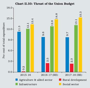 II.5.11 As per the latest information available, the fiscal position of the central government in terms of key deficit indicators deteriorated during the first quarter of 2017-18 (April-June) as compared to the corresponding quarter of the previous year. RD and GFD, both in absolute terms as well as per cent of BE, were higher than those in the corresponding quarter of the previous year. Deterioration in fiscal position was the outcome of lower growth in revenue and higher growth in expenditure. On the receipts side, growth in tax revenue decelerated sharply on account of a slowdown in all major taxes (income tax collections, customs duties, excise duty and service tax), except corporation tax. Total expenditure at 30.3 per cent of BE was higher than 25.9 per cent in the corresponding quarter of the previous year due to higher revenue expenditure and a sharp turnaround in the capital account – in conformity with the government’s intention of front-loading expenditure before the onset of monsoon. Going ahead, the pickup in capital expenditure augurs well for improvement in expenditure quality. 3. State Finances in 2016-17 II.5.12 Available information pertaining to 26 state governments indicates a deterioration in GFD, revenue and primary deficits in 2016-17 (RE) vis-à-vis the BE. The revenue account worsened because of shortfall in revenues and expenditure overshooting. Compared with the actuals of the previous year, the consolidated GFD increased by 0.4 percentage point to 2.9 per cent of GDP in 2016-17. 4. State Finances in 2017-18 II.5.13 The GFD-GDP ratio of states is budgeted to improve to 2.3 per cent during 2017-18 (from 2.9 per cent in the RE for 2016-17), largely on the back of a projected rise in tax revenue – both own tax revenue as well as tax devolution – and moderation in revenue expenditure (Chart II.34). The revenue account is also expected to post a surplus during the year. States have, however, a weak track record of fiscal marksmanship. Moreover, several risk factors such as implementation of their own pay commission recommendations and farm loan waivers may impact state finances in the near term (Box II.9). The flexibility for additional borrowings given by the 14th Finance Commission may encourage states to take greater recourse to market borrowings which, in turn, could exert pressure on yields, thereby raising the cost of borrowings. On the revenue side, the transition to GST may temporarily impact tax receipts, although the proposed compensation clause from the centre may provide some headroom (see Chapter III of the report on State Finances: A Study of Budgets of 2016-17). 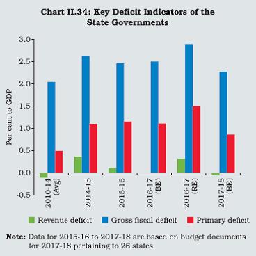
Box II.9
Farm Loan Waiver Recent instances of farm loan waivers in India include the Agricultural Debt Waiver and Debt Relief (ADWDR) Scheme announced by the central government in 2008 and state-specific farm loan waivers announced by Andhra Pradesh and Telangana in 2014; Tamil Nadu in 2016; and Uttar Pradesh, Maharashtra, Punjab and Karnataka in 2017, so far. While the benefit of debt relief to individual households can be substantial, the merit of unconditional bailouts in improving productivity and enhancing welfare remains debatable. While it has been argued that debt relief measures improve the productivity of recipient households as high levels of indebtedness distort investment and production decisions, the counter narrative suggests that loan write offs are detrimental to the culture of prudent borrowing and repayment and stigmatise borrowers in default. Moreover, they do not increase productivity of beneficiaries and affect households’ expectations about the reputational consequences of default leading to a decline in investment expenditure (Kanz 2012). In the Indian context, the ADWDR of 2008-09 was expected to benefit around 37 million small and marginal farmers and around 10 million other farmers. The cost of the Scheme was estimated to be about ₹717 billion (RBI 2008). In June 2016, the government of Tamil Nadu ordered the waiver of agricultural loans outstanding as at end-March, 2016 from co-operative banks to small and marginal farmers, the cost of which was estimated at around ₹60 billion over a 5-year period ending March 2022. The budgetary provision for the same in the form of grants amounted to ₹18 billion in the revised estimates for 2016-17 and ₹18 billion in 2017- 18 – both around 0.1 per cent of Tamil Nadu’s gross state domestic product (GSDP). A recent direction by the Madras High Court to the state government to extend the scheme to all farmers would further add to the state’s fiscal burden. In April 2017, Uttar Pradesh (UP) announced a farm loan waiver scheme which is expected to benefit small and marginal farmers by writing off their loans of around ₹360 billion – around 2.5 per cent of UP’s GSDP. Maharashtra has recently announced a loan waiver scheme for farmers; similarly, Punjab has announced a waiver on crop loans benefitting small and marginal farmers while Karnataka has announced a waiver amounting to ₹81.7 billion for farmers availing farm loans from cooperative banks. Implications First, the benefit of full loan waiver to farmers under the ADWDR of 2008 turned out to be highly skewed and concentrated in states where concentration of land holdings was low on account of land reforms (Ramakumar 2013). Second, waivers can have two major implications for the banking system: (i) while it may cleanse banks’ balance sheets in the short-term, it may disincentivise banks from lending to agriculture in the long-term (EPW Research Foundation 2008; Rath 2008); and (ii) farmers may tend to factor in future credit constraints and reluctance of formal institutions to lend to them following waivers; hence, they may tend to shift to informal sources of credit (Kanz 2012). Consequently, loan waivers can have a dampening impact on rural credit institutions. Moreover, they impact credit discipline, vitiate credit culture and dis-incentivise borrowers to repay loans, thus engendering moral hazard. Finally, loan waivers could add to the fiscal burden over the medium term as they are essentially a transfer from tax payers to borrowers. As per initial estimates, the total loan waivers announced during 2017-18 (upto August 2, 2017) amount around 0.4 per cent of GDP. Depending on possible cutback under other expenditure heads, this may result in an increase in the consolidated GFD-GDP ratio of states by about 20-40 basis points. An empirical exercise reveals that such random policy shocks have an enduring impact on market borrowings as evident from past episodes of such waivers. If overall government borrowings increase, yields on state development loans (SDL) may firm up posing higher interest burdens for states in the future. Concomitantly, they can also crowd out private borrowers as the general cost of borrowings increases with pressure from higher government borrowings on the finite pool of investible resources in the economy. An empirical exercise indicates that a one percentage point increase in the ratio of state debt issuance to GDP is associated with a decline of 0.067 percentage point in the ratio of corporate bond issuance to total assets of corporates. Thus, state government farm loan waivers have the potential to crowd out corporate borrowing if financed through state debt issuance. In order to understand the forces that drive loan waivers and their long term consequences for the entire economy, the Reserve Bank is organising a seminar on ‘Agricultural Debt Waiver-Efficacy and Limitations’ on August 31, 2017. References: 1. Rath, N. (2008), “Implications of the Loan Waiver for Rural Credit Institutions”, Economic and Political Weekly, June 14. 2. EPW Research Foundation (2008), “The Loan Waiver Scheme”, Economic and Political Weekly, March 15. 3. Kanz, M. (2012), “What Does Debt Relief Do for Development? Evidence from India’s Bailout Program for Highly-Indebted Rural Households”, Policy Research Working Paper 6258, World Bank. 4. Reserve Bank of India (2008), Annual Report 2007-08, Mumbai. 5. Ramakumar, R. (2013), “India’s Agricultural Debt Waiver Scheme, 2008”, Review of Agrarian Studies, 3(1): 135-146. | 5. General Government Finances8 II.5.14 The general government GFD is expected to be brought down further to 5.5 per cent of GDP in 2017-18 from 6.4 per cent in the revised estimates for 2016-17. This reflects the rigorous intent towards consolidation by the states. Outstanding liabilities of the general government are budgeted to decline to 62.7 per cent of GDP at end-March 2018 from 63.9 per cent at end-March 2017 (RE). Moreover, the debt servicing capacity of the general government has improved over the previous two years (Chart II.35). 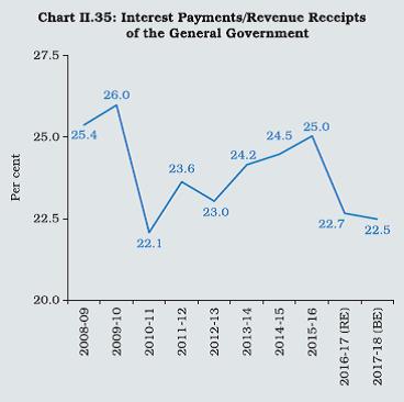 II.5.15 The central government’s fiscal strategy for 2016-17 was mainly revenue-driven, with buoyant tax collections comfortably funding additional expenditure commitments relating to the implementation of CPC and OROP awards, signifying the unswerving commitment to fiscal consolidation. At the state level, however, there was a slippage in FD, RD and primary deficit (PD) in 2016-17 (RE) along with a deterioration in debt position, partly due to their participation in UDAY. Going forward, GST remains the best bet for states in getting back to the path of fiscal consolidation over the medium term. The cushion of compensation by the centre for any loss of revenue in the initial five years should safeguard against uncertainty about the revenue outcome from the GST implementation. II.6 EXTERNAL SECTOR II.6.1 India’s external sector remained resilient in 2016-17 amidst considerable flux in the international environment; the Box in sub-section 6 on the external vulnerability watch argues the case analytically. Shrugging off a two-year contraction, merchandise exports turned around in the face of muted global demand. Drivers of this rebound are profiled in the immediately following sub-section. This development also assumes significance in view of the decline in net invisible receipts addressed in sub-section 3. Merchandise imports remained sluggish, although a significant pick-up occurred in H2. Consequently, rising international commodity prices and the erosion in terms of trade gains notwithstanding, India’s merchandise trade deficit narrowed further in 2016-17 and helped compress the current account deficit (CAD) as discussed in sub-section 4. II.6.2 Sub-section 5 discusses external financing and the predominance of non-debt creating inflows. Considerable volatility characterised portfolio investment flows against a backdrop of turbulent global financial markets and political risks. In contrast, direct investment inflows reached an all-time high. Net outflows were recorded under other major categories of financial flows barring trade credits which picked up in H2 in tandem with import activity. At the end of March 2017, India’s foreign exchange reserves covered for 11.3 months of imports and were the ninth largest in the world. 1. Merchandise Exports II.6.3 As global trade recuperated, and international commodity prices upturned, exports weathered transient disruptions in some labour intensive sectors and returned to a trajectory of persistent positive growth from August 2016, after a largely protracted decline (Chart II.36). While the modest recovery in global trade was driven by a pick-up in imports by emerging market economies (EMEs), India’s export recovery was largely led by shipments to advanced economies (AEs), notwithstanding the persistence of high tariff and non-tariff barriers in major trade partner economies (Chart II.37). 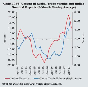
 II.6.4 The upsurge in exports in H2 spanned several commodity groups with a combined weight of 87.5 per cent in the export basket. The notable drivers were engineering goods, petroleum products, iron ore, cotton yarn, chemicals, marine products, gems and jewellery and readymade garments. A few of these sectors – petroleum products; iron ore; steel; cotton; and marine products – benefitted from a surge in international commodity prices. Exports of iron ore responded to strong demand from China. Steel exports accelerated sharply on the back of trade remedial measures, and underpinned the performance of engineering goods. Notwithstanding a transitory stress post-demonetisation, exports of labour intensive sectors such as readymade garments and gems and jewellery, quickly returned to expansion mode. Export recovery continued in April-June 2017 on the back of robust growth in engineering goods, petroleum products and readymade garments, though at a softer pace than Q4 of 2016-17. 2. Merchandise Imports II.6.5 Imports started picking up from H2 of 2016-17. However, they were largely sluggish in 2016-17, albeit with a marginal increase. Oil imports, in fact, turned around in 2016-17 in contrast to a large contraction in the previous year. On the other hand, there was a sharper reduction in gold imports and a slim increase in non-oil non-gold imports (Chart II.38). II.6.6 The expansion in the oil import bill occurred on the back of an increase in volume. International crude oil prices gradually firmed up through the year on a revival in the oil market sentiment, a temporary weakening of the US dollar, large supply disruptions and production cuts by the Organisation of the Petroleum Exporting Countries (OPEC). II.6.7 The volume of gold imports dipped by about one-fifth over the previous year. Strikes by jewellers against the one per cent excise duty, cash shortages following demonetisation, the income declaration scheme and high gold prices took their toll translating into a decline of 13.4 per cent in value terms. II.6.8 Non-oil non-gold imports remained muted for the year as a whole, even though a sharp pick-up was discernible across various commodity groups in H2 (Chart II.39). While the pick-up in demand for domestic coal reduced import volumes, the global surge in coal prices led to an increase in value terms. An uptick in imports of vegetable oil occurred on account of a modest increase in volume; however, this also reflected the uptrend in international prices. Imports of pearls and precious stones moved in tandem with higher exports of gems and jewellery. Import of pulses rose for the third consecutive year despite the highest ever domestic production, reflecting growing consumption and build-up of buffer stocks.  II.6.9 In contrast, a fall in raw material prices encouraged substitution of imports in the case of fertilisers, even though global prices softened sharply. Anti-dumping and safeguard measures undertaken by the government helped reduce steel imports significantly. With the improvement in the domestic production of capital goods, imports of machinery and project goods moderated. II.6.10 During April-June 2017, merchandise imports witnessed robust growth. While high growth in gold import volume contributed significantly to the increase in imports, oil and electronics imports also aided import growth further. 3. Invisibles II.6.11 Net receipts from invisibles, comprising services, income and transfers, declined during 2016-17 mainly due to moderation in software exports, private transfer receipts and higher net outgo on primary incomes (Chart II.40). In a phase of successive years of lowered global IT spending, domestic software companies faced pricing pressures in traditional services such as banking, financial services and insurance, and subdued growth in new businesses. Going forward, global headwinds for domestic software companies may intensify further with emphasis on local hiring, and higher demand for automation across major export markets. 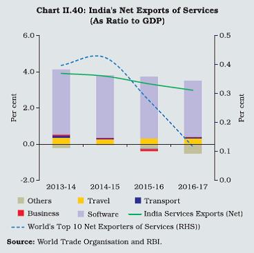 II.6.12 Net travel receipts increased by 5.3 per cent during 2016-17, as gains from higher tourist arrivals offset the burgeoning demand for travel services by residents. Under transfers, in-bound remittances to India were dampened for the second successive year by the weakening of growth and labour market “nationalisation” policies that impacted hiring of foreign workers in source countries. II.6.13 Net outgo with respect to profits and dividends also increased, largely reflecting higher returns that accrued to foreign investors on their investments in the domestic economy. In the aggregate, the net surplus from invisibles financed 86 per cent of the merchandise trade deficit, up from 83 per cent during the previous year, despite a contraction of 10 per cent during 2016-17. 4. Current Account deficit II.6.14 The bottoming out of international prices of major commodities in 2016 eroded gains in India’s terms of trade vis-à-vis the preceding two years (Chart II.41). Another downside factor that impacted the current account deficit (CAD) was the lower order of net receipts from services and remittances as well as higher outgo on income payments during 2016-17. Nevertheless, with the trade deficit shrinking on the back of stronger exports and subdued imports, CAD shrank to 0.7 per cent of GDP in 2016-17 as against 1.1 per cent a year ago (Chart II.42). 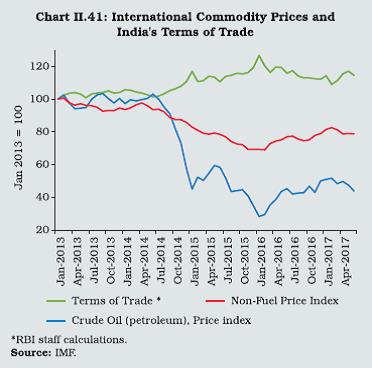
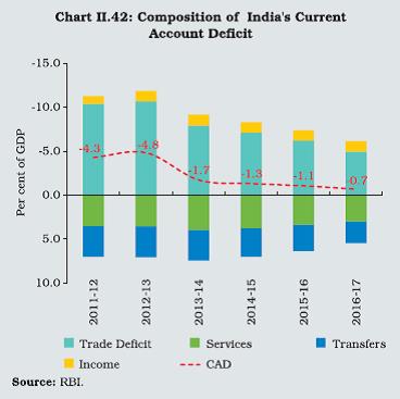 II.6.15 The gains in terms of trade realised in the preceding two years were slightly undermined by a modest upturn in international commodity prices in 2016-17. The erosion in terms of trade is estimated to have widened the merchandise trade deficit by 0.3 percentage point of GDP. The impact, however, was more than offset by compression in the trade deficit on the back of a recovery in export volumes and a modest decline in import volumes. Further, the positive impact of the trade volume also outweighed the negative contribution of software exports and remittances (Chart II.43). 5. External Financing II.6.16 Net capital flows were in excess of CAD, leading to an increase in foreign exchange reserves during 2016-17 to a level of US$ 370 billion by the end of the year (Chart II.44). Gross foreign direct investments (FDI) to India reached an all-time high of US$ 60 billion in 2016-17, up from US$ 56 billion a year before. This jump was catalysed by wide ranging domestic reforms, in particular, easing of FDI norms; the Goods and Services Tax; the Insolvency and Bankruptcy Code 2016; the new corporate insolvency framework, including the National Company Law Tribunal and the National Company Law Appellate Tribunal; and ease of doing business. Services topped the list of recipient sectors, followed by manufacturing and construction. A recent report by FDI Intelligence reveals that India was ahead of China and the US as the world’s top destination for greenfield FDI in 2016. Further, the UNCTAD’s survey of multinational enterprises ranked India as the third most favourite host country for FDI for 2017-19 after the US and China (Chart II.45). 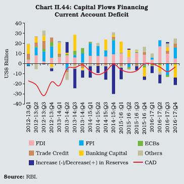
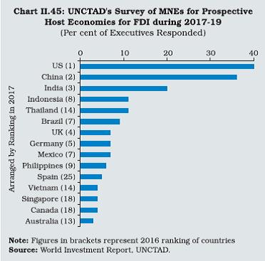 II.6.17 Foreign portfolio investment (FPI) flows remained volatile throughout the year. With the recovery in global equity markets on expectations of expanded monetary accommodation from systemic central banks, net FPI inflows were robust up to Q2. Subsequently, global risk aversion driven by the outcome for the US Presidential elections and expectations of an increase in the Federal funds rate, culminated in intense selling pressure in domestic equity and debt segments during November 2016 through January 2017. FPI flows (net), turned positive once again thereafter – aggregating US$ 23.4 billion during February to end-June 2017. II.6.18 Net inflows of short-term trade credit turned positive in H2 of 2016-17; this was in line with growing imports. In 2016-17, net inflows in the form of trade credit amounted to US$ 6.5 billion as against a net repayment of US$ 1.6 billion in 2015-16. Major sectors that took recourse to trade credit during the year included gold, oil, steel, edible oil and coal. II.6.19 External commercial borrowings (ECB) (net), recorded outflows on higher repayments. Even though ECB flows to India moderated in 2016-17, domestic companies took increasing recourse to rupee denominated bonds (RDBs) amounting to US$ 3,671 million as compared with US$ 14 million a year ago. The distribution pattern shows that one-third of the RDBs were raised for repayments of domestic rupee loans. About 41.0 per cent of the total ECB agreement amount (other than rupee denominated bonds/loans) was intended to be hedged as compared to 39.1 per cent a year ago. II.6.20 Notwithstanding positive accretions of deposits under Non-Resident (External) Rupee (NRE) accounts; and Non-Resident Ordinary (NRO) accounts, there was a net outflow of US$ 12.4 billion from non-resident deposits during 2016-17, following a lumpy redemption of FCNR (B) deposits raised by banks under the Reserve Bank’s special swap window during September to November 2013. In order to ensure a smooth redemption of FCNR(B) deposits, the Reserve Bank front-loaded liquidity provisions through open market operations and spot interventions/ deliveries of forward purchases. In the run-up to the redemption, the Reserve Bank took up short positions in the forward market for the US dollar, and reversed those positions during the redemption period. II.6.21 India’s external debt as at end-March 2017 stood much lower than a year before. This decline is mainly attributed to the fall in long-term external debt, particularly non-resident deposits reflecting the redemption of FCNR(B) deposits and commercial borrowings. As at end-March 2017, the share of US dollar denominated debt was 52.1 per cent of the total external debt, followed by the Indian rupee (33.6 per cent), SDR (5.8 per cent), Japanese yen (4.6 per cent), Euro (2.9 per cent), and others (1.0 per cent). 6. External Vulnerability Indicators II.6.22 India’s external sector vulnerability indicators are being monitored continuously. The configuration of a lower CAD, declining external debt, rising foreign exchange reserves and stable domestic fundamentals point towards greater resilience of the external sector in the recent period (Box II.10). The foreign exchange cover for external debt improved during the year while the share of short-term debt (residual maturity) in total external debt fell by over a percentage point, following the redemption of FCNR(B) deposits. India’s external debt to GDP ratio stood out one of the lowest amongst major peer EMEs (Chart II.46). 
Box II.10
Assessment of India’s External Sector Resilience India’s external sector parameters have improved over the last few years drawing strength primarily from a lower current account deficit (CAD). In general, a lower current account deficit augurs well for lower external financing requirements, build-up of reserves and a stable currency, albeit there could be other factors at play impacting each indicator separately. For instance, CAD, even if lower, financed through short-term debt may alter the composition of external debt and thus worsen reserve adequacy indicators. Hence, it is important to examine the external sector’s resilience in a more holistic manner by simultaneously focusing on key external indicators. With this background, two inter-related issues relating to external sector resilience were examined, viz.; (i) whether and, to what extent, the resilience of India’s external sector has improved over the period 2006-07:Q1 to 2016-17:Q4; and (ii) what the risks could be to the current level of resilience. Applying the Classification and Regression Tree Approach (CART) adopted by Lau et al (2003), data on five external sector indicators, viz., export growth, current account balance, net capital flows, reserve adequacy for short-term debt and the net international financial position were converted into probability-weighted “strong” and “weak” signs. Data points above (below) 80th (20th) percentile were assigned a probability of one of being a strong (weak) indicator. Data points within the 20th and 80th percentile were assigned probability depending on their relative closeness to either percentile values. Then, a decision matrix was drawn up to assign rating scores between 1 (weak) and 5 (strong) to each of the 32 possible combinations of the “strong” and “weak” signs of the five indicators. Finally, a fuzzy logic system was applied to the combinations to obtain an overall resilience score in a range of 1 to 5 (least resilient to most resilient) for each quarter. India’s external sector resilience score improved to 1.89 as at end-March 2017 from 1.54 as at end-March 2013, i.e., during the pre-taper talk period. However, the current resilience score is not only weaker than that of 3.68 at end-September 2008, i.e., just before the onset of global financial crisis but also, being closer to the lower end, it signals a general deterioration (Chart 1). For a robustness check, in an alternative specification, ‘export growth’ was replaced with the ‘terms of trade index’. The resilience score then improved marginally to 1.79 in March 2017 from 1.11 in the pre-taper talk period, but continued to be lower than the peak observed during the pre-global financial crisis period.  Weak exports, lower capital flows, higher net international financial liabilities and a lower reserve cover for short-term debt dragged down the current resilience score from the pre-global financial crisis period. However, all indicators except net capital flows/GDP were stronger during Q4 of 2016-17 than during the pre-taper tantrum period, thus translating into a higher resilience score. Even the recent improvement in the resilience score is subject to some downside risks. If terms of trade gains turn unfavourable in tandem with projected higher international commodity prices and the global demand conditions do not improve enough to support export volumes, CAD could increase due to a widening of the merchandise trade deficit. In fact, based on data for 1980-2016, it is estimated that a one per cent positive shock in terms of trade reduces India’s CAD by 0.03 per cent of GDP. Secondly, India’s software exports – a major source of financing merchandise trade deficit, face heightened uncertainty from protectionist policies being envisaged in advanced economies, especially with regard to H1B visa in the US, which may stress the current balance of payment (BoP). Thirdly, the short-term outlook for remittances flows to India largely depends on income conditions in source countries, especially the Gulf region which is facing low growth and undergoing fiscal consolidation, even though the assessment of the World Bank (2017) is more optimistic on this count. Finally, robust FDI inflows which were at the forefront in financing CAD in the previous three years, entail servicing through higher income payments which could have implications for CAD. References: Lau, Francis, Sunny Yung and Ivy Yong (2003), “Introducing a Framework to Measure Resilience of an Economy”, Quarterly Bulletin, Hong Kong Monetary Authority, June. World Bank (2017), Migration and Development Brief 27, April. | II.6.23 India’s net international investment position (NIIP) as a ratio to GDP improved, albeit the stock of foreign assets held by domestic residents (assets) and domestic assets held by foreign residents (liabilities) surged during 2016-17 (Table II.8). The dominance of FDI inflows over other forms of capital flows in recent years points towards a desirable qualitative compositional shift in India’s net international investment position. The share of non-debt liabilities increased to 50.3 per cent as at end-March 2017 from 46.3 per cent a year ago. | Table II.8: External Sector Vulnerability Indicators | | (Per cent, unless indicated otherwise) | | Indicator | End-Mar 2013 | End-Mar 2014 | End-Mar 2015 | End-Mar 2016 | End-Mar 2017 | | 1 | 2 | 3 | 4 | 5 | 6 | | 1. External Debt to GDP ratio | 22.4 | 23.9 | 23.9 | 23.5 | 20.2 | | 2. Ratio of Short-term to Total Debt (OM) | 23.6 | 20.5 | 18.0 | 17.2 | 18.6 | | 3. Ratio of Short-term to Total Debt (RM) | 42.1 | 39.7 | 38.5 | 42.7 | 41.5 | | 4. Ratio of Concessional Debt to Total Debt | 11.1 | 10.4 | 8.8 | 9.0 | 9.3 | | 5. Ratio of Reserves to Total Debt | 71.3 | 68.2 | 72.0 | 74.3 | 78.4 | | 6. Ratio of Short-term Debt (OM) to Reserves (%) | 33.1 | 30.1 | 25.0 | 23.1 | 23.8 | | 7. Ratio of Short-term Debt (RM) to Reserves (%) | 59.0 | 58.2 | 53.5 | 57.4 | 52.9 | | 8. Reserves Cover of Imports (in months) | 7.0 | 7.8 | 8.9 | 10.9 | 11.3 | | 9. Debt Service Ratio (Debt Service Payments to Current Receipts) | 5.9 | 5.9 | 7.6 | 8.8 | 8.3 | | 10. External Debt (US$ billion) | 409.4 | 446.2 | 474.7 | 485.0 | 471.9 | | 11. Net IIP (US$ billion)* | -326.7 | -340.8 | -364.3 | -359.5 | -392.9 | | 12. Net IIP/GDP ratio | -17.8 | -18.2 | -18.3 | -17.4 | -16.8 | | 13. CAD/GDP ratio | 4.8 | 1.7 | 1.3 | 1.1 | 0.7 | Note: OM: Original Maturity, RM: Residual Maturity, IIP: International Investment Position.
* (-) sign implies net claims of non-residents on India.
Source: RBI. | II.6.24 To sum up, India’s external sector benefited from lower CAD, robust FDI inflows, build-up of reserves and improvement in other vulnerability indicators. However, global factors continue to weigh on India’s external sector outlook. In particular, developments in the global oil market will have implications for India’s oil import bill. Further, India’s IT sector could face a challenging business environment from policy changes in the US which can affect its export potential. However, domestic macroeconomic fundamentals continue to remain strong, rendering the external sector resilient to global shocks.
|